Capsizing of Ships: Static and Dynamic Analysis of Wind Effect and
Cost implications
by
Angelos Antonopoulos
B.S., Marine Engineering, Hellenic Naval Academy, 1998
SUBMITTED TO THE DEPARTMENT OF OCEAN ENGINEERING I N PARTIALFULFILLMENT OF THE REQUIREMENTS FOR THE DEGREE OF
NAVAL ENGINEER and
MASTER OF SCIENCE IN OCEAN SYSTEMS MANAGEMENT at the
MASSACHUSETTS INSTITUTE OF TECHNOLOGY
JUNE 2006
O 2006 Massachusetts Institute of Technology. All rights reserved
The author hereby grants to MIT permission to reproduce and to
distribute publicly paper and electronic copies of this thesis document in whole o r in part
in any medium now known or hereafter created
I
t
...
Signature of Author:
...
.flaw. \Mechanical Engineering Department, Center for Ocean Engineering #
May, 12 2006
...
Certified by:
-
.
-
.
,
...
.-.. ..
; .T.7 ;...
d'
Jerome H. MilgramP r o f e s d M e c h a n i c a l and Ocean Engineering
v Thesis Supervisor
...
...
...
Certified by:
... ,.
,
V . ./
Patrick J. KeenanProfessopof the Practice of Naval Construction and Engineering Thesis Supervisor
-
...
.... .
...
...
Certified by:.,.
,.
,.
,0
Henry S. MarcusI n
/mp
/I
Professor of Marine Systemsn
Thesis SupervisorAccepted by:
...
(/,.
--
..
.' ..
.d....
Michael Triantafyllou Professor of Mechanical and Ocean Engineering Chairman, Department Committee on Graduate Studies
Capsizing of Ships: Static and Dynamic Analysis of Wind Effect and
Cost implications
Angelos Antonopoulos
Submitted to the Department of Ocean Engineering on May 12,2006 in Partial Fulfillment of the Requirements for the Degrees of Naval Engineer in Naval Architecture and Marine Engineering
And
Master of Science in Ocean Systems Management
ABSTRACT
Capsizing of small vessels, such as commercial fishing vessels, is a frequent event. This phenomenon is generally associated with the combined action of storm seas, inadequate design parameter regulations, and dangerous operational procedures. In contrast, the capsizing of large ships is rare, but does occur. For these large vessels, more strict regulations exist to ensure safe operational procedures. While the storminess of the sea cannot be controlled, the navigation procedure can. Large offshore ships tend to navigate in a path to avoid forecasted severe weather, and in cases of stormy seas they temporarily operate at safe speeds and in the direction parallel to the waves.
The work presented in this thesis investigates the effect of the wind in rolling and finally capsizing a ship. For the purposes of mechanical analysis, realistic hull forms are used and fundamental issues associated with moments and forces imposed by the wind, are applied. The platforms are examined for several wind speeds that strike the ship at different angles. Both static and dynamic cases were examined. Under the assumption of general conditions, the angles of heeling in each case and the wind speeds that caused the ship to capsize are calculated.
Furthermore, a cost analysis associated with the total loss of the ship due to capsize is also reviewed. An existing worldwide database of vessel total losses, dating from 1960 to present, is used to calculate the costs per ship capsize. Some simplifications are inevitably used, because the cost implications of total ship losses have both direct and indirect portions that are difficult to quantify. In addition, the actual numbers that result fiom such a catastrophe are not generally available to the public and are not found in the open literature. Given these limitations, a preliminary analysis of the capsize-associated costs is performed for several types of commercial vessels.
Thesis Supervisor: Jerome H. Milgram
Acknowledgments
First, I would like to thank my thesis advisors, Professors Jerome H. Milgram, Patrick J. Keenan and Henry S. Marcus for their valuable support and guidance throughout my studies. I would also like to acknowledge all the professors at the Ocean Engineering Department that contributed to my education. Finally, I would like to express my gratitude to the Hellenic Navy for financially supporting my academic pursuit.
Finally I would like to thank my friend, Georgios Constantinidis and my co-partner Marianne Holt-Phoenix whose reviewing and commenting was very helpful to me.
This work is dedicated to the memory of my father, Antonios, whose efforts and principles guided me through all my life. Also, it is dedicated to my mother, Eleni, and my brother, Haris, whose existence fill up my life
Table of Contents ABSTRACT
...
3...
ACKNOWLEDGMENTS 4 TABLE OF CONTENTS...
5...
LIST OF FIGURES 7 LIST OF TABLES...
8...
CHAPTER 1: INTRODUCTION 9...
CHAPTER 2: THEORETICAL BACKGROUND 11 2.1. MECHANISMS OF CAPSIZING ... 112.2. STABILITY CURVES INADEQUACY ... 12
2.3. FLOATING BODY PRINCIPLES AND RIGHTING ARM ... 12
2.4. HEELING ARMS ... 14
2.5. STATICAL STABILITY CURVES ... 16
... 2.5.1. Definition and Characteristic Points 16 ... 2.5.2. Dependency on the hull characteristics 17 CHAPTER 3: WIND EFFECT ON HULL
...
19. ... 3.1 HULL SELECTION 19 ... 3.2. CALCULATIONS SET UP 21 3.3. CALCULATIONS ... 2 2 ... 3.3.1. Projected Area Calculation 22 ... 3.3.2. Calculation of the force and the moment applied by the wind 23 3.3.3. Ship Righting Moment Calculation ... 26
3.3.3.1. Evaluation of roll angle in static case ... 26
... 3.3.3.2. Evaluation of roll angle in dynamic case 26
...
CHAPTER 4: SIMULATION RESULTS 31 ... 4.1. RESULTS WITH ZERO INITIAL CONDITIONS 31 ... 4.1.1. Tumblehome Hull Form 32 ... 4.1.2. Wall Sided Hull Form 34 ... 4.1.3. Flare-Sided Hull Form 36 ... 4.1.4. Discussion of the results 38 ... 4.1.5. Validation of the code 40 ... 4.1.5.1. Analflcal Solution 40 ... 4.1.5.2. Numerical Solution 43 4.2. RESULTS WHEN INITIAL CONDITIONS ARE NON ZERO ... 45... 4.2.1. Tumblehome Hull Form 46 ... 4.2.2. Wall Sided Hull Form 47 ... 4.2.3. Flare-Sided Hull Form 48 CHAPTER 5: FUTURE STEPS
...
49... . 5.1 UNIFORM WIND 49 ... 5.2. CD CALCULATION 50 ... 5.2.1. Model Set- Up 51 ... 5.2.2. Wind Characteristics 51 ... 5.2.3. Test Procedure 52
...
5.3. RISING OF WATERLINE AS THE SHIP HEELS 52
...
5.4. A44 B44 EXACT CALCULATIONS 55
...
5.5. FORCES AND MOMENTS APPLIED BY THE WAVES 55
...
CHAPTER 6: COSTS ASSOCIATED WITH CAPSIZING 57
6.1. CAUSES OF CAPSIZING ... 57
6.2. IDENTIFICATION OF THE COSTS ... 58
... 6.2.1. Costs Applied to the Shipping Industry 59 ... 6.2.1.1. Seafarers and Passengers 59 ... 6.2.1.2. Vessel Owners 59 6.2.1.3. Charterers 1 Shippers / Cargo Owners ... 60
6.2.1.4. Classification Societies ... 60
6.2.1.5. Shipbrokers ... 61
6.2.1.6. P&IClubs ... 61
6.2.1.7. Marine Underwriters ... 61
6.2.1.8. Banks and Financial Institutions ... 62
6.2.2. Costs outside shipping industry ... 63
6.3. VALUES OF SEVERAL DAMAGES
...
636.3.1. ValueofLife ... 63
6.3.2. Value of Damage to Property ... 64
6.3.3. Value of Environmental Damage ... 66
6.3.4. Value of Cargo ... 66
6.4. CALCULATIONS
...
686.5. ASSUMPTIONS & RJTURE STEPS
...
706.6. CONCLUSIONS
...
71REFERENCES
...
73APPENDIX I: DATA USED FOR THE CONSTRUCTION OF RIGHTING ARM CURVES
..
75APPENDIX 11: CALCULATION OF THE INTEGRALS FOR ADDED MASS MOMENT OF INERTIA. A44 AND DAMPING COEFFICIENT. B44
...
85APPENDIX 111: MATHCAD @ CALCULATIONS
...
89APPENDIX IV: MATLAB@ CODE
...
...
...
105APPENDIX V: TABLES OF ROLL ANGLES FOR ALL CASES WHEN INITIAL CONDITIONS ARE ZERO
...
...
113APPENDIX VI: TABLES AND FIGURES OF ROLL ANGLES FOR ALL CASES WHEN INITIAL CONDITIONS ARE NON-ZERO
...
119APPENDIX VII: DATA FOR BULK-CARRIERS LOSSES
...
131APPENDIX VIII: DATA FOR GENERAL CARGO SHIPS' LOSSES
...
....
137...
APPENDIX IX: DATA FOR PASSENGERS SHIPS1 ROROI CONTAINERSHIPS LOSS 161 APPENDIX X: DATA FOR TANKERS...
165...
APPENDIX XI: CALCULATION OF COSTS FOR SEVERAL TYPES OF SHIPS 171List Of Figures
FIGURE 1 : EQUILIBRIUM OF FLOATING BODY 13 FIGURE 2: ALTERNATE CONDITIONS OF THE EQUILIBRIUM OF A FLOATING BODY 14
FIGURE 3: EFFECT OF A BEAM WIND 15
FIGURE 4: CHARACTERISTIC POINTS ON A SHIP'S CURVE OF STABILITY 16
FIGURE 5: DEPENDENCE OF THE SHIP STABILITY CURVE ON THE HULL FORM AND SHIP MAIN DIMENSIONS 17 FIGURE 6: SCHEMATICS OF THE HULL FORMS EXAMINED 19 FIGURE 7: RIGHTING ARM CURVES FOR THE LARGE INITIAL METACENTRIC HEIGHT (GM=~.OM) 20
FIGURE 8: FIGURE OF DD(x) FOR THE CALCULATION OF PROJECTED TO THE WIND AREA 22
FIGURE 9: ANGLE OF ATTACK OF THE WIND WITH RESPECT TO THE SHIP 24
FIGURE 10: MOMENT APPLIED BY THE WIND ON A HULL 25
FIGURE 1 1 : TWO DIMENSIONAL STRIP THEORY FOR THE CALCULATION OF A44, B44 28
FIGURE 12: BEAM OF THE WATERPLANE AREA AS A FUNCTION OF SHIP LENGTH 29 FIGURE 13 : EQUILIBRIUM ROLL ANGLES FOR STATIC CASE (TUMBLEHOME GM= 1 . 5 ~ ) 32
FIGURE 14: MAXIMUM ROLL ANGLES FOR DYNAMIC CASE (TUMBLEHOME GM=1 .5M) 32
FIGURE 15: EQUILIBRIUM ROLL ANGLES FOR STATIC CASE (TUMBLEHOME GM=~.OM) 33 FIGURE 16: MAXIMUM ROLL ANGLES FOR DYNAMIC CASE (TUMBLEHOME GM=~.OM) 33 FIGURE 17: EQUILIBRIUM ROLL ANGLES FOR STATIC CASE (WALL SIDED GMZ1.5M) 34 FIGURE 18: MAXIMUM ROLL ANGLES FOR DYNAMIC CASE (WALL SIDED GM=1 .5M) 34 FIGURE 19: EQUILIBRIUM ROLL ANGLES FOR STATIC CASE (WALL SIDED GM=~.OM) 35 FIGURE 20: MAXIMUM ROLL ANGLES FOR DYNAMIC CASE (WALL SIDED GM=~.OM) 35
FIGURE 21 : EQUILIBRIUM ROLL ANGLES FOR STATIC CASE (FLARE SIDED GM=1 .5M) 36 FIGURE 22: MAXIMUM ROLL ANGLES FOR DYNAMIC CASE (FLARE SIDED GM=1 .5M) 36
FIGURE 23: EQUILIBRIUM ROLL ANGLES FOR STATIC CASE (FLARE SIDED GM=~.OM) 37
FIGURE 24: MAXIMUM ROLL ANGLES FOR DYNAMIC CASE (FLARE SIDED GM=~.OM) 37
FIGURE 25: DYNAMIC CASE MAXIMUM ROLL ANGLES FOR ALL HULL FORMS AND GMs AT @=go0 39 FIGURE 26: GRAPHICAL REPRESENTATION OF ANALYTICAL SOLUTION 43 FIGURE 27: GRAPHICAL REPRESENTATION OF THE NUMERICAL SOLUTION 44
FIGURE 28: COMPARISON FOR DIFFERENT INITIAL CONDITIONS (TUMBLEHOME GM= 1 .5M) 46
FIGURE 29: COMPARISON FOR DIFFERENT INITIAL CONDITIONS (TUMBLEHOME GM=~.OM) 46
FIGURE 30: COMPARISON FOR DIFFERENT INITIAL CONDITIONS (WALL SIDED GM=1 .5M) 47
FIGURE 3 1 : COMPARISON FOR DIFFERENT INITIAL CONDITIONS (WALL SIDED GM=~.OM) 47 FIGURE 32: COMPARISON FOR DIFFERENT INITIAL CONDITIONS (FLARE SIDED GMZ1.5M) 48 FIGURE 33: COMPARISON FOR DIFFERENT INITIAL CONDITIONS (FLARE SIDED GM=~.OM) 48
FIGURE 34 : WIND SPEEDS (KTS) AT VARIOUS HEIGHTS (M) ABOVE WL (NOMINAL SPEED 1 OOKTS AT 1 OM) 49 FIGURE 35: ARRANGEMENT FOR MODEL TESTS IN A WIND TUNNEL 51 FIGURE 36: PROJECTED TO THE WIND AREA AS THE SHIP HEELS 52 FIGURE 37: EFFECT OF THE RISING OF THE WATERLINE TO THE ROLLING OF THE SHIP 54
FIGURE 3 8: FAULT TREE FOR CAPSIZE 58
FIGURE 39: DEADWEIGHT PERCENTAGE OF TOTALLY LOST VESSELS PER SHIP CATEGORY 69 FIGURE 40: ~ L L E D / M I S S I N G PEOPLE PERCENTAGE DUE TO SHIP TOTAL LOSS PER SHIP CATEGORY 69
FIGURE 4 1 : MAXIMUM ROLL ANGLES FOR DYNAMIC CASE (TUMBLEHOME GM= 1 . 5 ~ ) 124
FIGURE 42: MAXIMUM ROLL ANGLES FOR DYNAMIC CASE (TUMBLEHOME GM=~.OM) 124 FIGURE 43: MAXIMUM ROLL ANGLES FOR DYNAMIC CASE (WALL SIDED GM=1 .SM) 125
FIGURE 44: MAXIMUM ROLL ANGLES FOR DYNAMIC CASE (WALL SIDED GM=~.OM) 125 FIGURE 45: MAXIMUM ROLL ANGLES FOR DYNAMIC CASE (FLARE SIDED G M = ~ . ~ M ) 126 FIGURE 46: MAXIMUM ROLL ANGLES FOR DYNAMIC CASE (FLARE SIDED GM=~.OM) 126 FIGURE 47: MAXIMUM ROLL ANGLES FOR DYNAMIC CASE (TUMBLEHOME GM=1 . 5 ~ ) 127 FIGURE 48: MAXIMUM ROLL ANGLES FOR DYNAMIC CASE (TUMBLEHOME GM=~.OM) 127 FIGURE 49: MAXIMUM ROLL ANGLES FOR DYNAMIC CASE (WALL SIDED GM=1 .SM) 128 FIGURE 50: MAXIMUM ROLL ANGLES FOR DYNAMIC CASE (WALL SIDED GM=~.OM) 128 FIGURE 5 1 : MAXIMUM ROLL ANGLES FOR DYNAMIC CASE (FLARE SIDED GM= 1 .SM) 129 FIGURE 52: MAXIMUM ROLL ANGLES FOR DYNAMIC CASE (FLARE SIDED GM=~.OM) 129
List of Tables
TABLE 1 : DYNAMIC CASE ROLL ANGLES AS A RESULT OF SEVERAL WIND SPEEDS AT 0 4 0 ' 38
TABLE 2: STATIC CASE ROLL ANGLES AS A RESULT OF SEVERAL WIND SPEEDS AT @=go0 38
TABLE 3 : TOTAL LOSSES OF SHIPS (1 989- 1999) 57
TABLE 4: DIRECT COSTS OF SHIP TOTAL LOSS FOR RESPECTIVE PARTIES 62
TABLE 5: CALCULATION OF COST PER FATALITY USING DIFFERENT ESTIMATIONS 64
TABLE 6: TOTAL OUTLAYS IN 2006 US $ FOR BULK CARRIERS (Ro-Ro, PASSENGER SHIPS, CONTAINERSHIPS
INCL.) 65
TABLE 7 : TOTAL OUTLAYS IN 2006 US $ FOR TANKERS (LNG, LPG INcL.) 65
TABLE 8: MAJOR COMMODITIES CARRIED BULK CARRIERS, CONTAINER AND GENERAL CARGO SHIPS 67
TABLE 9: MAJOR COMMODITIES CARRIED BY TANKERS AND LNGs 68
TABLE 10: CUMULATIVE DATA FOR SHIP ACCIDENTS PER TYPE FOR THE PERIOD 1960-2005 68
Chapter
1 :
I
ntroduct i on
7, 7. Prob lem Statement
Traveling at sea can result in casualties that lead to loss of life and money. Furthermore, in many occasions, maritime accidents can lead to serious environmental pollution. Fire,
explosion, collision, grounding, and/or machine~y breakdown are the main causes of ship
capsize and eventual sinkage, primarily due to loss of stability through reduction of reserve buoyancy.
Human factor is considered the most important cause of casualties at sea. This is usually encountered in the form of underestimation of several environmental conditions and ignorance of safety rules. Nobody can however ignore the significant role of the environmental conditions that a ship will face. Fog for example is an important factor that lowers the visibility and in many cases led to grounding or collision. Despite the many advances made in the area of radar and other electronic navigational aids, collisions and groundings continue to occur every year. It is hoped, however, that technological advances will in the near future reduce such occurrences.
Among the environmental factors that can cause capsizing of a ship or a boat, extreme weather conditions are dominant. In particular, the combined effect of wind and waves can lead to an excess roll angle, water on deck, or motion of the cargo. This vicious circle of chain events can eventually dnve the ship to capsize. Unfortunately, the capsize mechanism has not yet be fully understood due to the underlying complex dynamics and parameters. Despite today's advanced technology, it is not yet feasible to design and construct capsizing-resistant ships. The reason lies in the fact that it is not possible to model and simulate nature mathematically with all its aspects. Thus, the random, unpredictable, and sometimes chaotic character of ocean environment is responsible for capsizes and loss of life.
Studying the causes of capsizing in more detail, understanding the nature of waves and winds blowing over them, and finding the forces and moments that these conditions apply on the ship will contribute to a better understanding of capsizing phenomena. It is the intention of this thesis to contribute to the knowledge that can lead to the design of safer ships and the critical examination of existing vessels against capsizing.
7.2. Thesis
Out
1 ineThe aim of this document is to predict the roll angle that ships of a given hull form will suffer when subjected to winds of different velocities and angles of attack. In addition, this document will study the human reliability factor when decisions have to be made in order to avoid the capsizing danger when a heavy weather condition has been announced. Special attention is given to:
description of most important elements in each step of the prediction procedure major assumptions made and the limits of applicability
sensitivity of ship performance on the related parameters
This thesis is composed of six Chapters. The first Chapter deals with the presentation of the topic. Chapter 2 describes the theoretical background required to m e r investigate capsizing in ships. In particular it details the mechanisms of capsizing, the ship stability analysis, the generation of statical stability curves and how they are influenced by ship geometry (hull form).
Chapter 3 deals with the wind effect on hull. The three selected hull forms are tested under the influence of winds. The mathematical equations describing this phenomenon are developed and the theoretical predictions are presented. The effect of the wind striking the ship with different velocities and angles of attack during static and dynamic processes is investigated. The roll angle is calculated in all cases and conditions under which capsizing occurs are found.
Chapter 4 details the results obtained by the analytical formulation developed in Chapter 3. In order to properly solve the dynamic problem, initial boundary conditions are imposed. Apart fiom the case that the initial conditions are zero the chapter also includes calculations for the cases where non-zero initial conditions are experienced.
Chapter 5 summarizes the main assumptions made in this thesis and suggests potential routes for future refinements and increased accuracy.
Chapter
Theoretical Background
The purpose of this chapter is to give to the reader a quick general idea of some of the theoretical principles and background needed for the evaluation procedure that follows. All these theoretical aspects can be found in more details in any good naval architecture text.
2.
7. Mechanisms o f capsizingThe dominant cause of small ship capsizing is the combined action of breaking waves with excess magnitude winds blowing over them. Historical evidence suggests that small boats are more vulnerable to capsize due to breaking waves than large boats. In fact, capsizing of a vessel over 100 feet is very rare.
There are several mechanisms that can lead to capsize, some of which will be detailed below. Most of these mechanisms are essentially non-linear in nature and they cannot be investigated by a simple frequency-domain approach. One mechanism that can cause capsize involves static stability characteristics. In following or quartering seas, the wave- encountered frequencies are much lower than in head seas or seas on the bow, which means that the wave profile is almost stationary relative to the ship. As a consequence, the ship may become statically unstable in roll, relative to the waterline defined by the wave profile. This happens because the wave surface is not plane and neither is the
instantaneous load waterline. The metacentric radius BMT which is derived for this
modified waterline may in fact differ from that computed for the still waterline. The
metacentric height, GMT, is very sensitive to the metacentric radius and as a consequence
significant variations in GMT can occur with frequencies equal to the encountered
frequency. This parametric change of GMT can lead to roll instabilities, with roll motions
increasing in time. This effect is amplified for ships with low initial stability.
A different mechanism which can cause a ship to capsize, is a phenomenon called
broaching. As a term, broaching, describes the situation in which a ship veers broadside to the wind and waves. This can be caused when the fiequency of the encounter between the ship and the waves is small. The result is an altered course relative to the waves. This situation can lead to large amplitude of the unrestored motions of sway and yaw, which result in serious interactions with the steering and large resonant roll angles. In cases of extreme high waves and excess magnitude of winds, where the water particle velocities become comparable to the ship speed, the broaching mechanism may force the ship to yaw to an orientation parallel to the wave crest, which is extremely dangerous and may eventually lead to capsizing.
2.2.
Stab i I i ty Curves InadequacyIn order to investigate the safety of the ship-stability one needs to study its static and dynamic response under the effect of moments applied to the ship by winds and waves (or any other reason than can cause a heeling to the ship). The conventional statical stability analysis of ships is well known and simply presented by the righting arms (RA) curve. Unfortunately, the existing stability standards do not demand rigorous analysis of wave and wind forces that, often, are the main causes of capsizing. Various characteristics of the RA curve, such as the initial metacentric height, GM, angle of
vanishing stability, and area under the curve are directly dependent upon ship's hull form and weight distribution. This type of analysis should be extended a step fhrther to include the effect of external disturbing forces by wind.
To proceed to the wind effect analysis it is necessary to give a short introduction to the theoretical background of the ship stability. In particular, this section describes the importance of righting arms, the way that they are related to the angle of heel and their utilization for the following calculations.
It is known that a ship, as any afloat body, experiences the force of buoyancy equal to the weight of the displaced liquid. The resultant of that force is acting vertically upward through a point called the center of buoyancy (B), which is the center of gravity of the
displaced liquid. The application of this principle to a ship makes it possible to evaluate the hydrostatic pressure acting on the hull and the appendages by determining the volume of the ship below the waterline and consequently its centroid. This volume, when converted to weight, is called displacement (A).
The behavior of a floating object is determined by the interaction of the forces of the weight and buoyancy. In the absence of any other forces, and in the case of positive stability the ship will settle until the force of buoyancy equals the weight and it will rotate until the two following condition is satisfied, as shown in Figure 1
':
a. The centers of buoyancy B and gravity G are in a vertical line, and
b. Any slight rotation from this position from an initial waterline to another will cause the equal forces of weight and buoyancy to generate a restoring couple which tends to move the ship back to float on the initial waterline
Figure 1: Equilibrium of floating body
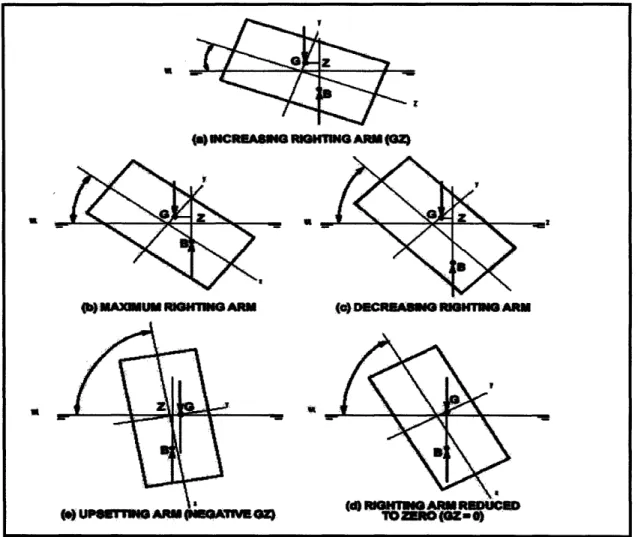
For every stable object there is at least one position at which the above conditions are satisfied. Any deviation fiom that position would produce a moment tending to restore the body to the initial position. These moments are called righting moments. Depending on the vertical position of the center of gravity, G, either righting moments which oppose further inclination or upsetting moments which contribute to continued inclination and potential capsize.
Lowering the center of gravity will increase stability. This happens because when a righting
arm
exists, lowering the center of gravity increases the separation of the two forces and thus increases the righting moment. When a heeling moment exists, lowering the center of gravity would change the heeling moment to a righting one. All the above are schematically shown in Figure 2*. To better understand the following figure, one needs to investigate how the righting arms change as the center of gravity is shifted along the y-axis.Figure 2: Alternate conditions of the equilibrium of a floating body
In addition to weight and buoyancy, there are other forces that may act on the ship. These forces are, generally, called upsetting forces and their magnitude determines the magnitude of the moment that must be produced by the weight-buoyancy couple in order to prevent capsizing or excessive heel.
External upsetting forces that can cause a ship-inclination may be: Wave action,
Wind, Collision, Grounding,
Shifting of onboard weights Addition or removal of weight High-Speed Turns
Towline pulls of tugs Entrapped water on deck
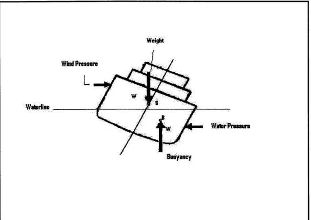
In the case where upsetting forces are acting on the ship, the ship heels to an angle whose value produces a moment by the forces of weight and buoyancy to equalize the moment developed by the upsetting forces. When the ship is exposed to a beam wind, the wind pressure acts on the portion of the ship above the waterline, and the resistance of the water to the ship's lateral motion is acting in an opposite direction in a point below the
waterline, as can be seen in Figure 33. As the ship heels from the vertical, the wind
pressure, water pressure and their vertical separation remain approximately constant. The ship weight is unchanged and acts at a fixed point. Even though the magnitude of the buoyancy remains the same, the point through which it acts depends on the angle of heel. Subsequently, equilibrium will be reached when sufficient separation of the centers of gravity and buoyancy has been produced to cause balance between heeling and righting moments.
Figure 3: Effect of a beam wind
In any of the cases when upsetting forces are applied it is quite possible that under several circumstances, equilibrium would not be reached before the ship capsized. It is also possible that the equilibrium would not be reached until the angle of heel becomes so
large that water would be shipped through topside openings, and the weight of this water would contribute to capsizing which otherwise would not have occurred.
2.5. S t a t i c a I S t a b i l i t y C u r v e s
2.5.1. Definition and Characteristic Points
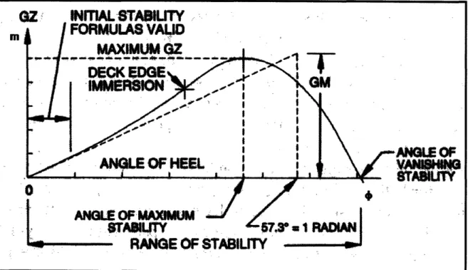
The statical stability curves are a plot of the righting arms or the righting moments of the ship against the angle of heel for a given condition of loading. For any ship, the shape of this curve will vary with the displacement, the vertical and transverse position of center of gravity, the trim and the effect of free liquids' surfaces. The area under the curve physically represents the potential energy that the ship possesses at corresponding heel angles. The standard plotting form of the righting arm curve is shown in Figure 44. In order to have a complete understanding of intact ship stability, it should be known not only how a righting arm curve is determined and used, but also why it is shaped as shown, and the significance of its typical features. The slope of the righting arm curve at zero is equal to the metacentric height of the ship. Up to about 5-10 degrees, the righting arm curve can be approximated by GZ = GMT sin($), where cp is the angle of heel.
Figure 4: Characteristic points on a ship's curve of stability
The peak of the righting arm curve identifies two quantities that are important in evaluating the overall stability of a ship. These are the maximum righting arm and the angle of maximum stability. The importance of the maximum righting arm is that when multiplied by the ship's displacement it produces the maximum steady-state heeling moment that the ship can withstand without capsizing. Beyond the angle of maximum
stability, righting arms decrease, often more rapidly than they had increased up to that
point. This rapid decrease, ultimately, leads to the point at which GZ becomes zero. The
angle at which this occurs is the angle of vanishing stability. Any ship that inclines beyond this angle will capsize. In reality, capsize could occur at smaller angles due to the additive heeling impulses posed by dynamic conditions.
2.5.2. Dependency on the hull characteristics
The shape of the righting arm curve depends heavily on the ship's hull form, both under and above the design waterline. While initial stability (righting arms at small angles of heel) depends almost entirely on metacentric height, the overall shape of the stability
curve is governed by hull form. Figure 55 shows how changing hull form increases or
decreases righting a m by altering the position and movement of the center of buoyancy.
Beam. Of all the hull dimensions that can be varied by the designer, beam has the
greatest influence on transverse stability. Metacentric radius (BM) is proportional
to the ratio B~/T. BM, and therefore KM will increase if beam is increased while
angle of deck edge immersion is decreased; righting a m s at larger angles and the range of stability are reduced.
Length. If length is increased proportionally to displacement, with beam and draft
held constant, KB and BM are unchanged. In practice, increasing length usually causes an increase in KG, reducing initial stability. If length is increased at the expense of beam, righting a m s are reduced over the
111
range of stability. If length is increased at the expense of draft, righting arms will be increased at small angles, but decreased at large angles.Freeboard. Increasing freeboard increases the angle of deck edge immersion,
increasing righting arms at larger angles and extending the range of stability. If draft is held constant, increasing freeboard causes a rise in the center of gravity, mitigating the benefits of increased freeboard to some extent.
Draft. Reduced draft proportional to reduced displacement increases initial
righting arms and the angle of deck edge immersion but decreases righting arms at large angles.
Displacement. If length, beam, and draft are held constant, displacement can be
increased only by making the ship fuller. The filling out of the waterline will usually compensate for the increased volume of displacement, and BM, as a
I x x
fimction of
-
,
will increase. The height of the center of gravity will also bev
decreased by filling out the ship's form below the waterline. These changes will enhance stability at all angles.
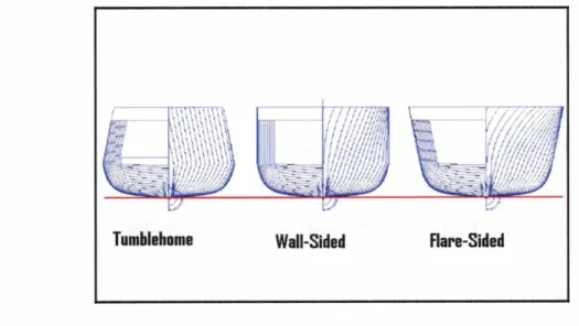
Side and Bottom Profde. Extreme deadrise (fining the bilges) or tumblehome in
the vicinity of the inclined waterline reduces the increase in waterplane area and outward shift of the center of buoyancy, resulting in a shallow stability curve. Ships with flaring sides develop large righting arms because of the rapid increase in waterplane area and large shift of the center of buoyancy as the ship is inclined. A round-bottomed ship with vertical sides beginning somewhat above the water line, such as a tug or icebreaker, will roll easily to small angles of inclination but develop strong righting moments at large angles.
chapter
3 :
This Chapter is devoted to the study of the wind effect on the heeling of a ship. To do so, we make use of the theoretical background described in Chapter 2. A code that calculates the roll angle that a ship experiences due to the moments applied from the wind which strikes a ship, is proposed. Particular emphasis is placed on tumblehome hulls due to the special interest expressed by several navies around the world to acquire and operate this type of ship. Tumblehome ships have the advantage of reduced electromagnetic signatures because the angled ship structure above the water line reflects the electromagnetic waves in a direction that makes the trace of the ship more difficult. However, a tumblehome ship will have decreased righting arms GZ, in the whole spectrum of the heeling angles and the angle of vanishing stability will also be lowered.
For the analysis and evaluation process three different hull forms were selected. A flare- sided, a wall-sided and a tumblehome. These types of hulls are schematically shown in Figure 66.
Tumblehome Wall-Sided Flare-Sided
Figure 6: Schematics of the hull forms examined
These hulls were developed under the supervision of the Seakeeping Division of the NAVSEA Warfare Center Carderock Division and the name of the project is
ONR.
TheRA curves for several values of initial metacentric height, GMT, were constructed. GMT
limits for safe operations at sea, using Sarchin and Goldberg criteriaare shown below: Tumblehome:
Wall-Sided: Flare-Sided:
For these values of GMT the righting arm curves versus the angle of heel were
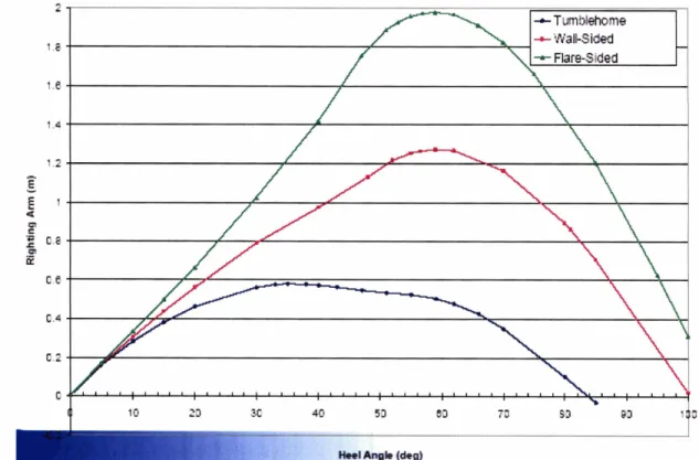
constructed by NAVSEA, and they are indicative of the superiority of the flare-sided
ships. These curves are shown in Figure 77
Figure 7: Righting arm curves for the large initial metacentric height (GM=2.0m)
While setting up the hulls to be examined, the following assumptions were made in order to make valid comparisons:
All of investigated hulls have the same principle characteristics L, B, T and the same displacement:
T=8.4 13m
A= 14264 ton
-
All of them have the same sail area. In other words, the heights of the ships' profiles above the waterline are assumed to be the same. This ensures that the forces applied by the wind and consequently the moments created are equal for all the types of the hull
The local drag coeficient was chosen to be one. (CD=l)
The velocity profile was uniform throughout the superstructure.
There are no other excitation forces applied to the hull of the ship apart from the wind force. Therefore, it is assumed that before any wind application the ship was in stillwater, and the initial angle of inclination and the initial angular velocity of the ship were zero
The waterline did not rise on the high side when the ship rolled, therefore the wind roll force and moment would be proportional to the square of the cosine of the roll angle
Discussion on how these assumptions will be altered will follow in proceeding chapter.
3.2. Ca/cu/atiuns
Set
upThe purpose of this work is to calculate and make finally a comparison of the following outcomes:
Find the forces and the moments applied on the hulls by the wind
Find the roll angle where the ship will balance after the application of the wind force for a long time. This will be called the static case
Find the roll angle that the ship will experience as a result of a wind that gusts causing a heeling angle greater than that found in static case. This will be called the dynamic case.
Finally, determine at which wind speed the ship will capsize, if any
The difference between the static and the dynamic case is the following. The static case evaluates the equilibrium roll angle for which the wind roll moment equals the ship righting moment. On the other hand, the dynamic case evaluates the extreme roll angle when the wind speed starts from zero and suddenly gusts to the prescribed wind speed which is maintained. In this case, the roll angle will overshoot the equilibrium value and as the ship behaves as a pendulum the energy provided by the wind will be absorbed by the ship restoring forces and finally the ship after a short period of time will be balanced to the angle calculated in static case.
This work will evaluate and plot the values of the angles described above for the following cases:
The three different hull shapes mentioned above
Two different righting arm curves for each hull with initial metacentric heights, GMF 1.5m and G M y 2 .Om
Several wind speeds in increments of 2 knots for values ranging in the region of 50 knots to 100 knots
The wind direction with respect to astern winds is called the angle 0. For the purposes of
this project, 0 would take the following values: 30°,450,600,900.~t is obvious that the
worst case scenario will be when the wind strikes the ship at an angle of 90'.
Subsequently, the values of the roll angles in the static and dynamic cases will be plotted as a function of wind speed in each of the wind directions, for the several hull forms and the two initial metacentric heights.
3.3. Calculations
3.3.1. Projected Area Calculation
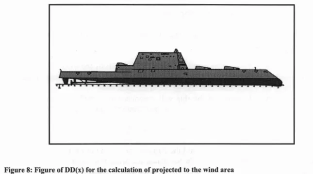
For calculation purposes, an existing preliminary design for the part of the ship above the waterline was used. This design is the DD(X) Multi-Mission Surface Combatant which is the future Surface Combatant for the US Navy.
Figure 8: Figure of DD(x) for the calculation of projected to the wind area
"DD(X) will be about 600 feet long, 79 feet wide, draw approximately 28 feet, and be
capable of speeds in excess of 30 knots. Displacement will be approximately 14,000 tons. The ship's tumblehome design will make it appear smaller than it actually is on radar. Although nearly twice the displacement of a Spruance-class destroyer, through signature reductions and its unique tumblehome hull design, DD(X) will be a stealthy warship and present a radar cross section a fiaction of Spruance-class ships."
Source: http://www . g l o b a l s e c u r i ~ . o r g / m i l i t a r y / s ~ m
Because the ship is not yet constructed, and because the design plans are confidential the
ship scheme given in Figure g8 was used. Knowing that the ship has an overall length of
about 600ft or 182.88m and measuring ship length from the figure, a ratio of the real ship and ship of the figure, called h was created. Using that ratio, and measuring the heights of the ship's profile in figure, the real ship profile heights can be estimated.
The profile of the projected area normal to the wind was represented by two single- column tables: one denotes the longitudinal position along waterline and another the corresponding heights. The table of longitudinal positions is in meters starting from x=Om at the stern of the ship and ending at x=182.88m at the bow. Because of the particular ship profile, the positions of measurements are not evenly spaced. Instead, the positions of measurements are selected according to hull profile changes. Both tables have 22 elements: 22 longitudinal positions, denoted as Lj and 22 corresponding heights, denoted as
Hj.
These tables can be found in Appendix 111.In a second step, we assume that j is taking values from 0 to 21, in order to cover all the longitudinal positions and heights. A function f(j) is defined to calculate the projected wind area of a small trapezoid between the positions
Lj
andLj+l
with corresponding heightsHj
andHj+l.
The whole projected area of the ship will then be given by the summation of all small trapezoids:
3.3.2. Calculation of the force and the moment applied by the wind
Another function of j, a(j19 is set to calculate the moment of area of each trapezoid about the waterline, and the sum of those will represent the first moment of the total projected wind area about the waterline, which is called
Mx:
1 ( H ~ ) ~
+
(Hj Hj + 1)+
(Hj + 1)'a(j) =-=(Hj+Hj+1)-(Lj.1-Lj).
Mx
divided by the Area will give the centroid of the area, Centroid,, with respect to the waterlineArea
The force on a surface can then be derived using:
where
CD is the local drag coefficient (CD=l.O),
pair is the air density (pair=l .2kdm3),
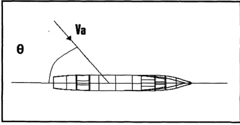
V, is the wind velocity in dsec., and
0 is the angle behveen the wind direction and the ship direction (0'
-
wind is coming fiomthe stern and 180'
-
wind is coming fiom the bow) as it is shown in Figure 9.The longitudinal fore-and-aft component of the wind has also some effect, due to the curvature of superstructure. The projected area to this component is very small compared to the projected area of the lateral component, thus the moment created fiom the horizontal velocity is negligible and can therefore be ignored. All following calculations do not take this horizontal component of the wind into account.
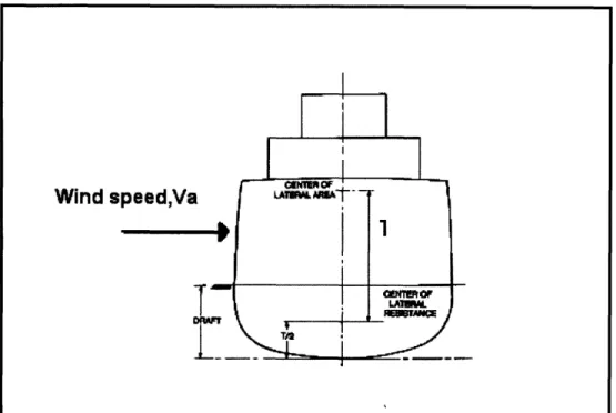
Another function of j, termed do), is set up to calculate the moment applied by the wind on each of the small trapezoids that constitute the hull. This moment will be equal to the product of the force applied on each piece and the lateral distance, 1, of the centroid of each piece from the point where the force from the water resistance is applied. It can be assumed that this point is at half draft, T/2. This issue is clarified in Figure lo1'.
Wind speed,Va
Figure 10: Moment applied by the wind on a hull
This formula is derived as follows:
where the total moment applied to the hull by the wind is the sum of all the moments applied to each trapezoid:
The force and the moment found using the above equations is what the ship experiences
in the upright position. As the ship inclines to some angle, cp, the force and the moment
applied on the hull is actually multiplied by a factor (cos2@ because in that case the wind
hits the ship in an angle cp so the ship realizes the Vaacos
4
component. Furthermore, in the expression giving the force and the moment applied by the wind (equations 6 &. 8), speed term is squared; consequently, the factor cos(cp) is also squared.3.3.3. Ship Righting Moment Calculation
Righting ann data for various heel angles was collected for each of the three hulls examined. This data ,collected from the ONR project, gives values of righting arms versus heel angle, GZ(cp), at initial metacentric heights of GM=l.Srn and GM=2.0m for tumblehome, wall sided and flare sided designs.
Since the ship used for the ONR project is similar to DD(x) but smaller (152.5m compared to 182.88), all the righting arms from the curves constructed for ONR are multiplied by a factor 1.2, which is the ratio of the DD(x) length over the ONR project ship's length. The decision to multiply with the ratio of the lengths and not the ratio of the displacements is made because the righting arms are measured in meters. Therefore it was proper to multiply with a ratio of a length scale, which is of the same dimension. A cubic spline was fitted to those points, in order to get a continuous function of GZ(cp) for that discrete characterization, as shown in Appendix I. This spline representation will help the MathCAD to use the function GZ(cp) in the equations that will give the static and dynamic solution for the roll angle experienced by the ship under wind effect.
3.3.3.1. Evaluation of roll angle in static case
For the static roll angle solution, a function T ( q ) is created. This function represents the difference between the moment applied by the wind,
[M
.
cos2#]
and the restoring moment of the ship, A GZ(4)The root of that function is the angle cp that will make both terms equal. This root will be the equilibrium angle that the ship will balance when is hit by a constant velocity wind.
3.3.3.2. Evaluation of roll angle in dynamic case
In an attempt to describe the complicated dynamic phenomena associated with ship
heeling, we represent the dynamic stability Up of a ship as the difference between the potential energies of the ship heeled at an angle g, and upright at 0 degrees. Since the work required to heel the ship by a differential dg, is
The total work required heeling the ship up to an angle q, or in other words, the dynamic
stability U, is expressed by:
The dynamic stability is therefore directly proportional to the integral under the righting
arm curve. When the external moment by the wind which is a fbnction of 9, M
.
cos24
,
isapplied, the ship's equation of motion, taking into account that water is acting as a damper to the rolling of the ship, becomes:
with initial conditions:
where:
A44 represents the moment of inertia of the ship around the roll axis and equals the
squared radius of gyration, k:, multiplied by the ship displacement converted in
kg to match the units
A 4 4 represents the added mass moment of inertia of the hull around the roll axis
B44 is the roll damping coefficient
C4 is the restoring force coefficient and has the value of the displacement,
converted in mass units, multiplied by the gravity acceleration g
,
(C44=A g)Because the offsets of the hulls studied for the purposes of this research are not known,
the only known value in equation (12) is C4. The values AM, &, B44 will be calculated
making some assumptions. The value that can be calculated most readily is AM making the assumption that the radius of gyration is one third of the beam of the ship.
For
h4
and BM the following procedure will be followed:Step 1: It is known that if the sectional added mass, ~ 1 4 4 and b44 is given for each section
of the ship at any position-x then integration of this along the length of the ship will give,
consequently, the values of A 4 4 and B44. The sectional added mass terms, c 4 4 and b44, can
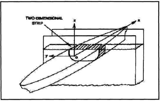
be found by solving the 2-D hydrodynamic problem shown in Figure 1 1 "
.
Figure 11: Two dimensional strip theory for the calculation of
w,
b44Then, using strip theory the values of the added mass terms for the whole ship, A44 and B4, can be determined by using the following equations:
Step 2: As the exact offsets of the ship are not known, the exact calculation of sectional coefficients, ~ ~ 4 4 and bM is impossible. The use of experimental results is necessary. Using Figure 46 on p.62 of PNA (Principles of Naval Architecture Volume 111) we can obtain a non dimensional sectional added mass moment of inertia and damping coefficient in roll for a rectangle of beam B and cross-sectional area A, as a function of non-dimensional frequency of the motion. A mean value fiom these charts is chosen as:
The purpose of this thesis is not to derive the exact values of the added mass terms but to predict the roll angles experienced by the ship under high speed winds in the dynamic case. Because the added mass moment of inertia is very small compared to the moment of inertia of the ship and because doubling the damping coefficient will change the maximum roll angle by less than four percent, we can assume the validity of the above
values from the chart given in PNA. In the following step, a method of finding the added moment of inertia and the damping coefficients of a slender body when sectional coefficients are known in any position of the ship will be presented, for future reference.
Step 3: Using Figure 1212 that shows the waterplane area of the DD(x) at draught
waterline, a function of the half-beam of the ship can be obtained.
Pos: x=182.88 Pos : x=69.494 Pas:O
Figure 12: Beam of the waterplane area as a function of ship length
So the function of the half-beam of the ship with respect to the longitudinal position (bow defined as x=O) is given from the following formulas:
B = 0 . 1 7 3 4 4 6 * ~ for
0
5 x 5 69.494mB = 12.0548 for 6 9 . 4 9 4 m ~ x ~ I 8 2 . 8 8 m (15)
Assuming that draft remains unchanged for the entire length, the cross-sections of the ship will be rectangles of different beams and same drafts with an areaA =
B w T .
Therefore combining the equations (13), (14), (15), A44 and BM can be written down as:The solution of the above integrals in order to obtain a value for the 4 4and B44 terms is
shown in Appendix 11. A factor of two at the integrals exists for calculate A44 and
B4
for the whole ship as the hnction B is giving the half beam.This step is created to generate a reasonable procedure of getting these coefficients and it can be used as a reference in fbture utilization, when the sectional added mass terms and the offsets of the ship are known exactly.
Inputting the values of A44, B44 and C4, the MATHCAD 1 2 0 gives the function of the roll angle versus time, cp(t). Given these values and the capabilities of the program, a maximum roll angle when the wind gusts fiom zero to the prescribed value, is calculated. After a long period of time (P>O), the roll angle should coincide with the static roll angle.
Both the static and dynamic roll angle calculation procedures for all the cases examined are shown in Appendix 111.
chapter 4: simulation ~ e s u l
t s
4.1. R ~ S U 7ts with zero i n i t fa 7 conditions
This chapter presents the simulation results as predicted by the model proposed in Chapter 3. The need to obtain roll angles for a) static and dynamic cases, b) three different hull types, c) two different initial metacentric heights, d) four different wind angle of attack, and e) twenty six wind speeds in the range of 50 to 100 knots in steps of two knots, produces a large number of required simulations (1248 combinations) that would be very tedious to run manually in the MATHCAD 1 2 0 code.
In order to accommodate this large number of runs, a MATLAB0 code is developed that uses the equations described in Chapter 3 to statistically and graphically obtain the roll angle values for all described cases. This code is included in Appendix IV. The validity of the MATLAB0 code was verified by cross checking the results that each program gives for certain cases.
Tables of the roll angles of ship heeling for both static and dynamic cases for each hull form and each initial metacentric height for all the combinations of wind speeds and directions are presented in Appendix V.
In what follows, the results for static and dynamic cases are presented in graphic format. The x-axis and y-axis in the graphs represent the wind speed in knots and the roll angle in degrees, respectively.
At the end of this section a table and a graph for the worst-case scenario (this happens at beam winds [8=90*]) are also constructed which will help to make the comparison.
4.1.1. Tumblehome Hull Form
0 1 , , , , , , , , , , , , , , , , , , , , ; , , , , , 1
Wind Speed Va (knots)
''
'"''II
Figure 13: Equilibrium roll angles for static case (Tumblehome GM=l.Sm)
Wind Speed Va (knots) 91 knots
Wind Speed Va (knots) " - '
Figure 15: Equilibrium roll angles for static case (Tumblehome GM=2.0m)
Wind Speed Va (knots)
I
I
a x i m u p ~ o & n ~ d p a m i c . q-f,r case --- (Tumblehome --- - ---.7-,- GM=2.Om),- - , - --, -. - .
4.1.2. Wall Sided Hull Form 18 16 14
3
g! 12 m5
10-
-
8=60 aa I- -
.
e=45E
8a
-
e=30 I 6dt
4 2 0 50 60 70 80 90 100Wind Speed Va (knots)
Figure 17: Equilibrium roll angles for static case (Wall Sided GM=l.Sm)
70 80 90
Wind Speed Va (knots)
I' I
14 12
3
10t
'
8=
-
-
8 ~ 6 0 Q, I a 6-
-
.&45C
I-
8
4 2o . . .
50 60 70 80 90 100Wind Speed Va (knots)
Figure 19: Equilibrium roll angles for static case (Wall Sided GM=2.0m)
I I
Wind Speed Va (knots)I I
I' I
4.1.3. Flare-Sided Hull Form
70 80 90
Wind Speed Va (knots)
Figure 21: Equilibrium roll angles for static case (Flare Sided GM=l.Sm) 1.
70 80
Wind Speed Va (knots)
Wind Speed Va (knots)
I 1
Figure 23: Equilibrium roll angles for static case (Flare Sided GM=2.0m)
70 80
Wind Speed Va (knots)
4.1.4. Discussion of the results
As can be seen fiom Figure 13 through Figure 24 as well as fiom the data presented in
Table 1 and Table 2, the tumblehome ship of initial metacentric height of 1.5m will
capsize if it will experience a beam wind gust of over 90 knots. In reality, there is a possibility that capsize will occur earlier. The maximum righting arm appears at an angle of inclination of 28 degrees. Since the MATLABO code doesn't break down until the
wind speed becomes 91 knots, it can be accepted, for the purposes of this thesis, that the
ship will withstand beam winds up to 91 knots.
T a b I: Dynamic case roll angles as a result of several wind speeds at
Wind Speed (kts)
I08
Tumblehome for GM=I.Sm 7.34 11.63 17.51 26.21 40.17 Capsize
Tumblehome for GM=2m 5.35 8.1 1 11.68 16.07 21.19 27.39
Hull Form Wall Sided for GM=I.Sm 7.39 10.79 14.99 20.22 26.14 32.25
Wall Sided for GM=2m 5.29 8.02 11.21 14.58 18.44 23.05
Flare Sided for GM=1.5m 7.41 10.42 13.95 17.99 22.37 26.85
-- - - -
I
Flare Sided for GM=2.0 m1
5.681
8.021
10.741
13.871
17.341
21.021
Table 2: Static case roll angles as a res
L - . - - L
. a - n - - - ' .
Flare Sided for GM=I.Sm 3.97 5.52 7.34 9.39 11.71 '. :t14.33
Flare Sided for GM=2.0 m 3.01 4.24 5.67 7.28 9.08 11.08
It is obvious from a comparison between Table 1 and Table 2, that when a ship receives a wind which is gusting fiom zero up to a nominal speed the ship will heel at a maximum angle which is almost twice as much as the angle of equilibrium. Provided that the wind
continues to blow at this nominal speed for some periods of oscillation, the ship will remain heeled at an angle equal to the angle of equilibrium which is found under the
study of static case.
F7.,
XIy,J@qg& ;::. I
- #41a.r 7,. &, - !; ;.;73?rPY,>2T:$ a' 8 X -<& I ' ; . L ' L . l01"~!. ' - fii : j 9 I, i
i
, # I it .. 6 8 e~tm$&jal*
- ;,ki.~d : . ,A
r -----
- -,---
--- +. -w--. -. ----&+-.+---- L.p-.-r.ru.- A . 7 , --..-".I2 ---, -A -J ,50 45 40 35 A cn
#
30 W a l l s i d e d [GM=2.0m]8'
-Wall Sided [GM=I .5m]=
-
-Tumblehome [GM=2.0m] o, 25 I m-
-Tumblehome [GM=I .5m] c a F l a r e Sided [GM=I .5m] 20 PL -Flare Sided [GM=2.0m] 15 10 5 0 40 50 60 70 80 90 100 110 Wind Speed Va (kts)Figure 25: Dynamic case maximum roll angles for all hull forms and GMs at O=!loO
Figure 25 presents the maximum roll angles obtained for the dynamic case for the range of speeds fkom 50 knots to 100 knots for all the different hulls examined. It can be observed that in the case of initial metacentric height of GM= 2.0m, the difference between the three different hull forms is less than the difference observed for the GM= 1.5m case. For both cases, however, roll angles in the vicinity of wind speeds of 50 knots are essentially the same but they tend to deviate as the wind speed is increased. It should be noted that in the case of the initial metacentric height of 1.5m the deviation is much bigger than the deviation occurs with initial metacentric height of 2.0m.
In any case, as it can be understood by graphs and table, the flare sided ship is superior in terms of stability. Wall sided ships are less stable, while the tumblehome ships show the least desirable stability under high winds' effect.
As claimed by NAVSEA experiments on tumblehome hulls, the adequate metacentric height for a ship of this kind to be stable is 2.0m and more. This is also confirmed by the presented calculations.
The graphs presented in paragraphs 4.1.1-4.1.3 demonstrate that the roll angles decrease as a ship veers in a way to reduce the wind angle of attack to less than 90'. The reduction of the angles of roll becomes greater as the angle between the wind and the ship is reduced. Consequently, a ship which is going to experience bad weather conditions has two options: one is to try to avoid the weather if time permits and the other, if there is no time to avoid the weather, is to keep a course as parallel as possible to the direction of the blowing wind.
Also, it must be mentioned that a ship will capsize from combined effect of wind and waves. In the above calculations only the effect of the wind is given. In reality with both wind and waves, capsize will occur in much lower wind speeds.
4.1.5. Validation of the code
4.1.5.1. Analytical Solution
This section is devoted to validation of the MathCADO code. In order to do so we investigate a special case where analytical solutions exist and compare the results with the numerical solution given by the code. The dynamic case problem, expressed by equation (12), can be solved analytically for very small angle of heeling. This relates to the physical scenario that small heeling moments are applied to the hull of the ship by the wind.
In that case equation (12) can be written in the form:
where we use the approximation for small angles: cos2
4
=
landGZ=GM.sin(4)=GM*+
Using an initial metacentric height of 2.0m, a wind speed of 10 knots that should produce a small heeling moment ( M I O = 5.75 1 -lo5 ~ m ) and the values for A44, h 4 , B44 and C44, as they can be obtained from Appendix 111, equation (17) becomes:
This linear second order differential equation can be solved analytically using simple mathematics. The roll angle as a function of time is given by:
The graphical representation of this function of time can be obtained by any mathematical software and it has the shape of Figure 26:
e ,
' , ' ' Figure 26: Graphical representation of analytical solution
,. 1 .
-
.
4.
-. . . .- . -
_.
. _ I.
. , .The red line in the figure above represents the roll angle as a function of time, while theI ' ,' - . I
. I - ' . + . 'blue and green dashed lines represent the envelope that encloses the roll angle function. .-. The dashed lines physically represent the roll angle amplitude decay ratio. For input
.
. : -.
Itvalues of cosine in equation (20) of 1 and -1 the green and blue lines take the analytical- . - -
'-' ' d : forms
Ml0
(1
+
eo.0185r ) and Ml0 (1-
e 0.0185t ),
respectively.r
, GM C44 GM *CM , ., ,. PJ
.
.
' ..
+.
1.; )id!-' &- ; -. . . . - . .
k .
om equation (1 9), it can be derived t h a M 0 . 5 5 3 radi econd and
) I, , 1,
..
2 . z
- - . - -' .
-.
. ' therefore the natural period of the system is:Tn
= - = 1 1.362 sec.
Of great value is alsoWn
- .4 . .
. - . . . - - - 1
the time scale
-
= 54.05 sec over which the oscillatory part of the roll amplitude - 7 '. -. . _ _ .. .. 0.01 85 . " , . ,-- ., .,; > .;i , - 1 , r ! : ! : - - . # . ,.:-
>.,'.I7 A T # . , ? 1.
*- 7 * - a w , ,;.3ePQBd
' - . 8 .. : . : --..willdecaybyafactor-.3
.--3
L
- I- e-
.
. . . .@'F6'.:.
'>: , -. . . - .6 1 w i h f ~ ~
,: . + . 4.1.5.2. Numerical Solution . . . -. - . -. . .
2 . ' , .The MalchCAD code was also used, for the tumblehome ship with initial metacentric
height GM=2.0m. The equation used for that run can be found in Appendix 111 and is also
.
, - . . .. given below: . . d . - 4 . - b I.
1 - L S. . - '. '. . '. . . . ,-.' a .:.
I , :.
. . . . ...
7:,<,.:. . I -!, , *; . .<.. + L :. . - ., - , 1.
. , . . . . ,. . - ., ., .:. + ,.
..#-..
,; . L. ,' .,,,,., - .,;, : , - . < ! ..: ,; ;' . ' I . . ; ' . . . ' . ' .'I ' T . L ., . - ' a . .; * . h , .: < r , .,*..
.. . _ . . . - . I -I - .,. .
4 ' ;.'. 1 . . . 8 ..
. . . ..
. . . ! .. .
- , . . b - . . ..
- ,.
r - . 8 . 4 . . . . ._ .. , . A 7 \! ... , ' ,-.
. .. - . . . h . . . ..
! , :: , . . . ' . 8 .a ..
T...
.. -
* I,' . . :. ' .'. . . .'. . . . i :. -. , 2 I - . . ' . . < . . , . - . . - .. m . - .., 7 I .4 . :.
L . ,. I .I.:, , , . . I , ' '- >. - '.
, I . - -.-
. . ..
1.
C , ' . ,L' . r :.. ' . . , _ ' . . . ' " - . . . . . .. _ . - A - .where II(cp) is the cubic spline created to fit the righting arm curve.
The MathCAD solution to this non-linear equation is graphically represented in the form
of the roll angles versus time, in Figure 27:
Figure 27: Graphical representation of the numerical solution
. . . . . . A comparison between the numerical and analytical results demonstrates:: :
For long equilibrium times (t =1000secs) the code suggests a roll angle of 0.127
degrees, while the analytical solution gives a roll angle of -. . .
lim[ M1o (1
+
e".0185t)I
=O. 13, a discrepancy on the order of 2.3%.GMDC44 , . . .
..','r. .
From the graphs one can obsiee that -iflir 200 seconds the n&ber of cycles will
. .
be equal for both cases. . .
..*
The local first maximum can also be evaluated for both cases. The maximum roll- angle can be directly derived from the analytical and numerical roll angle
functions, which turn out to be 0.225 and 0.242, respectively, thus an error of 7%.
These small deviations between numerical and analytical predictions can be attributed to the cubic spline approximation which only approaches reality in the vicinity of small
positive angles. In fact, the tangent of the cubic spline at zero is smaller or greater than the initial metacentric height depending on the case.
4 , 2 , ~ e s u 7 t s when i n i t i a 7 conditions are non zero
All calculations and graphs assume that the ship, before the wind gusts, was at rest, which means that the sea was calm and the initial angle of heeling and the initial angular velocity were zero. This however, is not realistic. A ship moving on the waves will gain some angle of inclination or some angular velocity under several circumstances. The following two case studies examine the results for dynamic case rolling angles when (I) there is an initial angle of inclination (caused i.e. by a turning of the ship or an angle imposed by damage) and (11) initial angular velocity (caused i.e. fiom a wave striking the ship from the side and providing the energy to the ship to start oscillation). These two cases intensify the problem if the application of the moment applied by the wind is in the same direction as the initial angular velocity or the initial angle of heeling. This will contribute to the generation of larger rolling angles and the reduction of the maximum wind speed that the ship can withstand without capsizing.
For the purposes of these case studies, the MATLABO code created in previous steps, is used to run the combination of each hull form and each of the two initial metacentric heights for a range of speeds fiom 50 knots to 100 knots in increments of 2 knots. For the first case study an initial angle of six degrees of inclination is assumed. For the second case study an initial angular velocity of 0.1 radfsec is examined. Those two values cannot describe the real and complex nature of movements of the ship in a rough sea, and they are arbitrary, but they are indicative of the deterioration of ship stability.
Tables and graphs of the resulting maximum rolling angles for both case studies in each of the above mentioned combinations are presented in Appendix VI. In the following sections, a comparison of the results for each hull and each initial metacentric height for the worst-case scenario of beam winds [0=90°] is presented. The resulting graphs show that for all types of hull, and both initial metacentric heights, the ship becomes more vulnerable to capsize in the dynamic cases where the maximum roll angles are bigger for the whole wind velocity range when initial conditions are applied. [0=90°].
4.2.1. Tumblehome Hull Form TUMBLEHOME GM=l.Sm 45 A 40 30
z
CONDITIONSy
25 I N I T I A L ANGLE OF HEELg
20a
15 =INITIAL ANGULAR Jd
10 K 5 0 40 60 80 100 WlND VELOCITY (kts)Figure 28: Comparison for different initial conditions (Tumblehome GM=l.Sm)
TUMBLEHOME GM=2.0m 45 40 A
8
35 30 25 CONDITIONS-INITIAL ANGLE OF HEEL