Detection strategy for long-term acoustic monitoring of blue whale stereotyped and non-stereotyped calls in the Southern Indian Ocean

HAL Id: hal-02398789

https://hal.univ-brest.fr/hal-02398789

Submitted on 8 Dec 2019

HAL is a multi-disciplinary open access

archive for the deposit and dissemination of

sci-entific research documents, whether they are

pub-lished or not. The documents may come from

teaching and research institutions in France or

abroad, or from public or private research centers.

L’archive ouverte pluridisciplinaire HAL, est

destinée au dépôt et à la diffusion de documents

scientifiques de niveau recherche, publiés ou non,

émanant des établissements d’enseignement et de

recherche français ou étrangers, des laboratoires

publics ou privés.

Detection strategy for long-term acoustic monitoring of

blue whale stereotyped and non-stereotyped calls in the

Southern Indian Ocean

Maëlle Torterotot, Flore Samaran, Jean-Yves Royer

To cite this version:

Maëlle Torterotot, Flore Samaran, Jean-Yves Royer. Detection strategy for long-term acoustic

moni-toring of blue whale stereotyped and non-stereotyped calls in the Southern Indian Ocean. OCEANS

2019 MTS/IEEE, Jun 2019, Marseille, France. �10.1109/OCEANSE.2019.8867271�. �hal-02398789�

Detection strategy for long-term acoustic

monitoring of blue whale stereotyped and

non-stereotyped calls in the Southern Indian Ocean

Ma¨elle Torterotot

Laboratoire G´eosciences Oc´ean Universit´e de Brest & CNRS

Brest, France

maelle.torterotot@univ-brest.fr

Jean-Yves Royer

Laboratoire G´eosciences Oc´ean Universit´e de Brest & CNRS

Brest, France jean-yves.royer@univ-brest.fr

Flore Samaran

Abstract—The most common approach to monitor mysticete acoustic presence is to detect and count their calls in audio records. To implement this method on large datasets, polyvalent and robust automated call detectors are required. Evaluating their performance is essential, to design a detection strategy adapted to study the available datasets. This assessment then enables accurate post-analyses and comparisons of multiple independent surveys. In this paper, we present the performance of a detector based on dictionaries and sparse representation of the signal to detect blue whale stereotyped and non-stereotyped vocalizations (D-calls) in a larg acoustic database with multiple sites and years of recordings in the southern Indian Ocean. Results show that recall increases with the SNR (Sound to Noise Ratio) and reaches 90% for positive SNR stereotyped calls and between 80% and 90% for high SNR D-calls. A detailed analysis of the influence of dictionary composition, SNR of the calls, manual ground truth as well as interference types and abundance, on the performance variability is presented. Eventually, a detection strategy for long term acoustic monitoring is defined.

Index Terms—blue whales, bioacoustics, detection, perfor-mance evaluation, long term monitoring

I. INTRODUCTION

Blue whale (Balaenoptera musculus ssp.) acoustic repertoire is composed of two sound types: stereotyped calls and variable down-sweep calls, named D-calls hereinafter [1]. The former are repeated periodically by males only, over long periods of time, up to days, to form songs [2]. Each sub-species and population produces its own song, composed of spe-cific calls [3]. Although their time-frequency shape is highly stereotyped, the pitch of tonal parts of many population calls is globally decreasing [4]. While the causes for this long-term frequency decrease are still unclear, a seasonal variation seems to be linked to the ambient noise level [5]. D-calls are low frequency down-sweeps, ranging from about 90 Hz to 30 Hz and lasting from 1 to 8 seconds, produced by males and females [7]. Unlike stereotyped calls, their time-frequency shape and duration are highly variable, and their occurrence is sporadic. D-calls have been recorded in the presence of blue whales in the Pacific [1], [8] and in the Atlantic [9], of Antarctic blue whales [10], [11] and of three acoustic

populations of pygmy blue whales in the Indian Ocean [12]– [14].

Easier to detect automatically, stereotyped calls are com-monly used to monitor blue whale sub-species and population presence and migrations. Yet, the presence of blue whales in the Pacific has been attested by the occurrence of D-calls, whilst no stereotyped calls were detected [8], [15]. Besides, D-calls appear in the behavioral context of foraging [7], whereas songs are thought to be a reproductive display. Thus, monitoring both call types brings insights not only on blue whale migratory routes, but possibly on their breeding and feeding grounds.

In this paper, we use a detection method based on dictionary learning and sparse representations of stereotyped and non-stereotyped calls [16], [17]. The detector works with dictionar-ies built from temporal call signals and then considers variabil-ity in those calls by using sparse representations; hereinafter, it will be referred as a sparse representation detector or SRD. Preliminary tests on small datasets demonstrated the potential of this detection algorithm on Madagascan pygmy blue whale calls and Pacific blue whale D-calls [16]. However, before applying this detector to a larger dataset, it is imperative to thoroughly evaluate its performance and analyze its variability to develop a detection strategy that will allow meaningful interpretations and potential comparisons across different stud-ies [6], [18]. Moreover, detection performance are needed to estimate accurate cetacean densities from passive acoustic data [19].

Performances are often determined by comparing the de-tector outputs with a ground-truth dataset, generally obtained by a manual annotation of a subset of the global dataset. Detection and false-alarm rates are two common metrics to measure these performances. Ideally, these metrics should be constant and independent from the selected data subset, so that the measured performances are representative for the entire dataset. In practice, as shown for instance for detections based on spectrogram correlations [18] , the following factors can impact the detection performances: variability in the call characteristics, seasonal call abundance, ambient noise and

human analyst variability. The latter factor has been inves-tigated in detail for Antarctic blue whale call detection, where independent manual annotations of identical datasets exhibited strong variability between analysts, which in turn reflected on the detection performances [6]. This variability illustrates the difficulty to reliably and reproducibly identify single calls in a whale chorus made of overlapping distant calls. Before performing automated detection on large datasets, it is also necessary to define if, how and which interfering acoustic signals may affect the performance of the detector. Once all these precautions are taken, an accurate detection strategy can be set up.

This paper investigates the performances of SRD before its application to detect diverse blue whale calls on a long-term dataset collected in the Southern Indian Ocean. Section II presents the methodology used to detect blue whale calls and to evaluate the detector performance in the available dataset. Section III focuses on the performance assessment. Finally, section IV discusses the results and how the detection strategy must be adjusted to investigate multiyear databases.

II. MATERIAL ANDMETHODS

A. Data collection

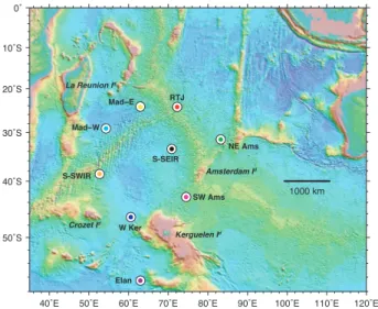
This study is based on acoustic data recorded by the OHASISBIO (Observatoire Hydro-Acoustique de la SISmicit´e et de la BIOdiversit´e) hydrophone network, deployed in the Southern Indian ocean since 2010 [20]. This array is composed of 5 to 9 moorings, depending on the year, and covers a region spanning from 24° to 56° South and from 52° to 83° East (see Figure 1). Each mooring is composed of an anchor, an acoustic release and a hydrophone, moored at the depth of the sound fixing and ranging (SOFAR) channel. The recordings are continuous and sampled at 240 Hz.

Kerguelen Id

Amsterdam Id

La Reunion Id

Crozet Id

40˚E 50˚E 60˚E 70˚E 80˚E 90˚E 100˚E 110˚E 120˚E

50˚S 40˚S 30˚S 20˚S 10˚S 0˚ 1000 km Mad−W S-SWIR W Ker SW Ams NE Ams S-SEIR RTJ Mad−E Elan

Fig. 1. The OHASISIBIO hydrophone network in the Southern Indian ocean. Colored dots represent mooring sites.

Two blue whale sub-species dwell in this area: the Antarctic blue whale (B. m. intermedia), referred hereinafter as Ant BW, and the pygmy blue whale (B. m. brevicauda), among which

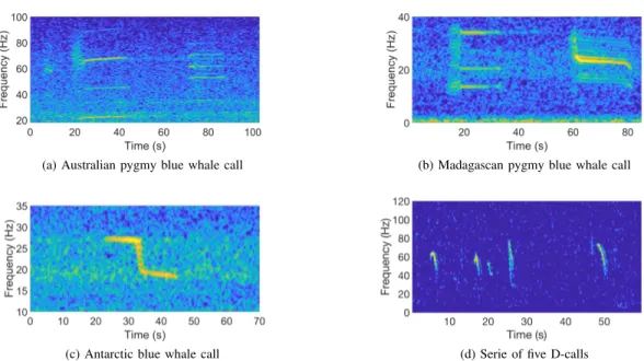
two acoustic populations are clearly identified in our acoustic records: the Madagascan (Mad PBW) and the Australian (Aus PBW) pygmy blue whales [21]. Each of these sub-species emits a distinctive and stereotyped call and possibly common or unrelated D-calls, as pictured on Figure 2.

B. Selected data subsets

Performances of the detector are evaluated on small subsets of this passive acoustic data. For the purpose of this study, three subsets have been created.

1) Data subset 1: To compute the performance metrics on interference-free data, four subsets (one for each call type) were built. Audio files were chosen to cover a large range of acoustic scenarios: from calls with high SNR to calls barely visible among the chorus, a din noise made of overlaid distant calls. For stereotyped calls, only data from 2015 were selected, to be invariant to the long-term call pitch shift [5]. For the data subset with D-calls, records were chosen among the whole OHASISBIO dataset, to account for potential geographical and temporal variability in the call type. A total of 240.5 hours of recordings were selected for the D-call data subset, 110.5 hours for Aus PBW, 78 hours for Mad PBW and 58.5 hours for Ant BW.

2) Data subset 2: This dataset will serve to evaluate the effects of the analyst ground-truth on the detection perfor-mances. Data selection process was similar to that of dataset 1, but with no overlap between the two datasets. However, the size of the three subsets for Mad PBW, Aus PBW and D-calls, are much smaller (6-hour long), so that multiple analysts could annotate them. Moreover, no Ant BW subset was built for this analysis.

3) Data subset 3: Once the performances were assessed on interference-free datasets, the detector was applied on one year of recording at site WKER. This site was chosen based on a manual inspection and previous analyses of the data that established the presence of the different call types [22]. The objective is to characterize the interferences that could lure the automated detection and to re-evaluate the false alarm rate in case of call absence.

C. Manual annotation

Manual annotation is solely considered for data subsets 1 and 2, as this is a long and tedious task that can only be achieved on small datasets.

1) Data subset 1: Manual annotation was made with Raven Pro 1.5 (Cornell Lab of Ornithology). Spectrograms with fixed parameters (Hanning windows with 50% overlap and 512-point FFT) were visually inspected by an expert human operator. Each call type was annotated one at a time. Only unit 2 of Aus PBW call and unit 1 of Mad PBW call were logged while for D-calls and Ant BW calls, the whole call was selected. Each manual detection was saved into a text file (beginning and end-time), to be compared with the automated detector outputs. A total of 3467 D-calls, 1697 Aus PBW calls, 2000 Mad PBW calls and 1499 Z-calls from Ant BW were logged by the analyst.

(a) Australian pygmy blue whale call (b) Madagascan pygmy blue whale call

(c) Antarctic blue whale call (d) Serie of five D-calls

Fig. 2. Spectrogram of blue whale calls used to assess performance of the detector. (a) Australian pygmy blue whale stereotyped call (b) Madagascan pygmy blue whale stereotyped call (c) Antarctic blue whale stereotyped call (Z-call) (d) Serie of 5 D-calls

2) Data subset 2: Multi-analyst manual annotation was completed using the Aplose online annotation platform devel-oped by the Ocean Data Explorer project [23]. This platform can be remotely accessed by multiple analysts and displays spectrograms with fixed parameters (Hanning windows with 80% overlap and 512-point FFT). Four expert analysts anno-tated D-calls and three of them annoanno-tated stereotyped calls, all with the same annotation protocol as for data subset 1. D. Pre-processing of the data

Before detection, the audio files are whitened using a FIR filter whose time-varying impulse response is derived from the noise power-spectral-density estimated every 300 seconds as described in [24, Appendix A]. This process makes the detection insensitive to the different types of background noise encountered in the dataset. Data are then bandpass filtered in the call frequency bandwidth reported in Table I. For stereotyped calls, data are also converted into baseband signals, with the frequency bounds reported in Table I, to reduce processing time.

TABLE I

FREQUENCY BANDWIDTH OF CALL TYPES USED FOR DETECTION Call type Frequency bandwidth (Hz)

D-calls 30 - 90

Mad PBW calls 35 - 45 Aus PBW calls 62 - 72 Ant BW calls 16 - 28

E. Detection method

The detector is based on dictionary learning and sparse representation of blue whales vocalizations. The principal asset of this method lays in the alliance of big dictionaries, that take

call variability into account, and linear combination of several elements of those dictionaries, to reflect call complexity. The detection principle is thoroughly described in [16].

Practically, detection is conducted in 2 steps :

1) Dictionary creation: dictionaries are directly designed from the data. Given a set of L time-based signals s, K-SVD algorithm [25] seeks the dictionary D, of size M_{6 L, that leads} to the best possible representation for each signal in this set. Here, signals s of calls can well be represented by a linear combination of a small number K of non-zero coefficients in the basis D. K is called sparsity constraint and is directly related to the complexity of each single call type to detect. If Kis over-evaluated, the number of false detection will tend to increase. On the contrary, if K is under-estimated, the detector may miss true detections. The dictionary size M has to be large enough to depict the variability of the calls, but must also stay small to limit computing time. In this study, the size of the dictionary M and the sparsity constraint K have been taken from reference [17]: for the highly variable D-calls M = 45 and K = 3, and for the stereotyped calls M = 20 and K = 2.

2) Detection: The algorithm scans the acoustic data by bins of N samples, equals to the duration t of the calls composing the dictionary. For D-calls, t = 8 s, for Aus PBW calls t = 25 s, for Mad PBW calls t = 20 s and for Ant BW calls, t = 18 s. The Orthogonal Machine Pursuit (OMP) algorithm then seeks the linear combination of K elements among the M dictionary elements that best matches the observed signal. In other words, for an observation vector y and a known dictionary D, the algorithm estimates θ as the approximate solution of

min

θ∈RM||y − Dθ||

2

Then the following threshold test, τη(y) =      1 if ||Dθ||22 ||y−Dθ||2 2 > η 0 otherwise, (2)

with τη(y) the decision metric and η the detection threshold,

is performed. τη(y) can be interpreted as a measure of the

Signal to Interference-plus-Noise Ratio (SINR) with ||Dθ||22

an estimate of the signal of interest and ||y −Dθ||22an estimate

of the interference-plus-noise [16]. A detection is considered to be true only if the SINR is above the threshold η (see Section III-A for an explanation threshold choice).

F. Performances evaluation

Performances are tested in three steps, each one operated on a data subset presented in section II-B. The first step aims at appraising the detector performance on a controlled, interference-free dataset. The second step assesses the perfor-mance variability due to the annotator ground-truth data. The last step will test the performances against data variability, such as the presence of interferences, or various call abundance scenarios.

1) Step 1: The main goal is to determine the average detection and false-alarm rates for stereotyped calls and D-calls. In order to do that, two datasets are extracted from the manually annotated calls of data subset 1: a training set, used to build the dictionary, and a test set, used to evaluate the performances. Usually, the learning set is made of a greater percentage of calls (at least 60 %) of the dataset than the test set. However here the purpose of the method is to detect calls from a large database with a limited amount of calls that define the dictionary. Therefore, the training set is made of less calls (50 for stereotyped calls and 200 for D-calls) than the test set. Evaluation of performance is assessed by comparing the detector outputs from the test set, with the ground truth detections established by an experienced human operator. Automated detections can be either true positive, when the detected call matches with a manually annotated call, i.e. when the midpoint of the time of the automated detection falls within the time bounds of the manual detection and vice versa; or false positive, when the detector detects something that has not been logged by the expert analyst. Detection rate, also named recall, is defined as the proportion of true calls found by the automated detector against the total number of calls in the manually annotated data set:

Recall = Number of true positive

Total number of call in the ground truth. (3) The number of false alarm per hour, or false-alarm rate, is the ratio between the number of false positive and the duration of the dataset in hours.

False alarm rate = Number of false positive

Dataset duration (in hours). (4) The second goal is then to evaluate the robustness of the detector by doing some cross validation, i.e. to test whether

the detector performance is dictionary dependent or not. Per-formances are computed multiple times on the same dataset by using the k-fold cross validation method to constitute the training and test sets. Mean and standard deviations are then computed for analysis.

2) Step 2: The second step is to assess the performance variability due to the analysts’ manual annotation of the data. The dictionaries used by the detector are built from one of the step 1 training set. Detector outputs are compared to the ground truth built by the multiple analysts. Detection and false-alarm rates are then averaged and standard deviations computed for the three call types.

3) Step 3: To examine the effect of interferences and call abundances on the automated detection, the detector is tested on a larger dataset made of the acoustic data recorded at site WKER in 2015. The dictionaries used by the detector are the same as in step 2. Here, a detection rate cannot be reported, since a manual ground-truth of a whole year dataset would be time consuming and tedious to establish. Yet, a false-alarm rate can be quantified by checking and classifying the detector outputs: a detection is declared as true when the detection is indeed a call, or false when the output is an interference. The interferences are then manually sorted into categories, according to the types occurring the most regularly.

III. RESULTS-PERFORMANCE EVALUATION

In this section, performance and their variability are evalu-ated for stereotyped and non-stereotyped blue whale calls on three data subsets of the OHASISBIO hydroacoustic data. A. Performance evaluation on data subset 1

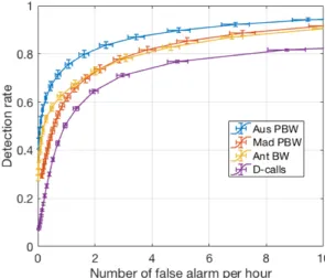
Figure 3 represents the Receiver Operating Characteristic curves for all call types detection done on data subset 1. These curves represent the average detection rate as a function of the average false alarm rate, both estimated for the k test sets. The number of false alarms per hour is determined by the detection threshold η. Best performances are achieved when

Fig. 3. Receiver Operating Characteristic (ROC) curves for the three blue whale stereotyped calls and D-calls

the detection rate is maximized for the smallest false alarm rate possible. The detector seems to perform better on stereotyped calls, with a detection rate at least 10% higher than on D-calls, regardless of the false-alarm rate. Even among stereotyped calls, detection rates are variable with a higher detection rate for Aus PBW at constant false alarm rate. To evaluate the effect of the Sound to Noise Ratio of the calls on detection performance, Figure 4 displays the detection rate of all call types for a fixed threshold η set to -8.2 for Aus PBW, -8 for Mad PBW, -9.1 for Ant BW, and -11.6 for D-calls, which correspond to an average false-alarm rate of 1.15/h, 1.06/h, 1.06/h, and 0.96/h, respectively. For each noisy observation y of a call, the SNR is estimated in the call bandwidth reported in Table I as

SN R = y

T_y

N σ2 − 1, (5)

where y is the call signal and σ2 is given by the robust estimator detailed in [24, Appendix A].

Fig. 4. Detection rate as a function of the Signal to Noise Ratio of the calls. The false alarm rate is set at 1 per hour for all the calls.

Detection rates increase with the SNR of the calls and be-come greater than 95% for stereotyped calls with a SNR above 5 dB. A variation in recall is observed within stereotyped calls and the detector performs globally better on Aus PBW and Ant BW calls than on Mad PBW calls. Overall, for D-calls, recall is lower and reaches a plateau between 80% and 90%, even for high SNR calls.

B. Performance evaluation on data subset 2

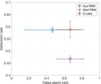
Detection was performed using dictionaries build in step 1 and detection threshold are defined as above. Means and standard deviations of the detection and false-alarm rates are illustrated in Figure 5. Average detection rate of Aus PBW and Mad PBW calls both reach 0.58 but with a wider standard deviation for Mad PBW calls (±0.01 and ±0.03 respectively). Mean recall values for D-calls is lower than for stereotyped calls (0.47±0.01). All false alarm rate values are below one

per hour with lower value for Aus PBW calls (0.46±0.32) than for Mad PBW and D-calls (0.67±0.15 and 0.67±0.15 respectively).

Fig. 5. Recall and false alarm rate (mean and standard deviations) for three call types, determined by comparing the detector outputs with tdifferent ground truth built by three analysts.

C. Performance evaluation on data subset 3

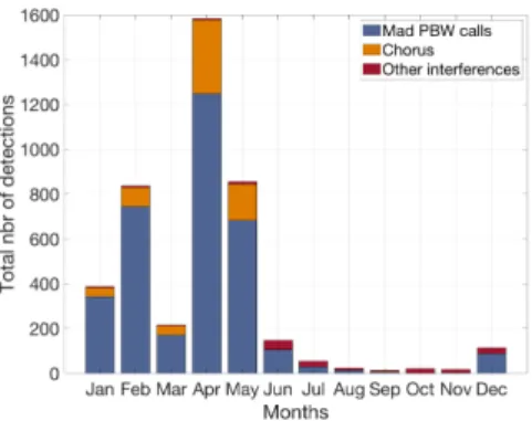
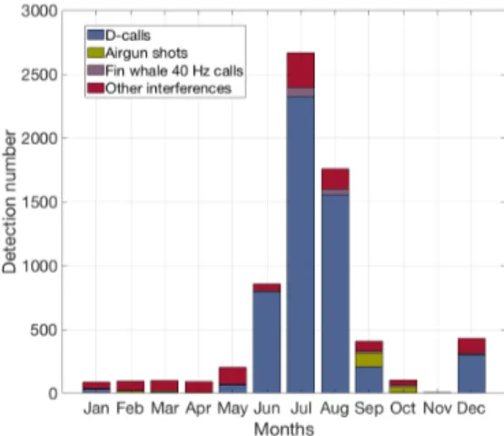
Long-term detections on WKER 2015 site are summarized in monthly histograms for each of the four calls (Figure 6). Detection patterns are highly seasonal with detection peaks in austral autumn for both pygmy blue whale acoustic pop-ulations and in winter and spring for Antarctic blue whale calls and D-calls. For stereotyped calls, the number of false alarm is far below the theoretical one false alarm per hour. This number is consistent over the year and therefore over different call abundance scenarios. Most interferences are due to chorus, especially for Mad PBW calls. Other interference types include ship noise and undetermined continuous banded noise in the call frequency bandwidth. For D-calls, the false alarm rates and types are very variable depending on the months. Two main categories of interferences have been identified: air gun shots and fin whale 40 Hz calls. The former are impulsive broadband sounds that are emitted periodically every 10 seconds during seismic surveys. The latter are thought to be social sounds produced by fin whales. They fall in the same frequency band as D-calls but they are more impulsive with a duration below one second; their spectrograms are compared in Figure 7. Other types of interference are mostly broadband short sounds and their occurrence seem constant over the month.

IV. DISCUSSION/CONCLUSION

Evaluating detector performances is essential to allow the correct use and interpretation of passive acoustic data [18]. Multiple sources of performances variability of SRD are investigated in this study, including call type, composition of the dictionary, SNR, ground-truth manual annotation as wall as interference type and abundance. Then, taking these

(a) Australian pygmy blue whale call detections for WKER 2015

(b) Madagascan pygmy blue whale call detections for WKER 2015

(c) Antarctic blue whale call detections for WKER 2015 (d) D-calls detections for WKER 2015

Fig. 6. Detection patterns as found by the detector at site WKER in 2015. (a) Australian pygmy blue whale call detections (b) Madagascan pygmy blue whale call detections (c) Antarctic blue whale call detections (d) D-call detections

(a) Air gun shots

(b) Fin whale 40 Hz calls

Fig. 7. Spectrogram of the two main types of interferences mistaken for D-calls by the SRD

observations into consideration, a detection strategy for long-term monitoring is presented.

A. Call type, SNR and dictionary composition effects on the detection performances

An efficient detector must combine high recall with low and consistent false alarm rates. Here, for a predetermined false alarm rate, the detector appears to generally perform better on stereotyped calls. Indeed, while detection rate reaches almost 95% for high SNR stereotyped calls, it doesn’t exceed 85% even for very high SNR D-calls. This trend is also observed in reference [26], where the detection performance are better for Ant BW stereotyped calls than for D-calls and in reference [27] where false alarm rate is particularly high for an average recall. D-calls, are highly variable but simple down-sweep signals, that can easily be mistaken for any kind of transient noise, often very abundant in underwater acoustic soundscapes (e.g. seismic shots). This may explain why most algorithm fail at identifying them, even when they have a high SNR.

Detection performances are also variable among stereotyped calls. If on the ROC curves in Figure 3 the detector seems to perform better on Aus PBW, Figure 4 actually shows that performances are equivalent for Aus PBW and Ant BW calls. But because the proportion of calls with a SNR below -5 dB is more than twice higher in the Ant BW dataset than in the

Aus PBW dataset, the overall performances are lower for Ant BW calls. For similar SNR bins, recall of Mad PBW is lower than for the two other stereotyped calls. The OHASISBIO dataset is characterized by the presence of an important chorus, especially in the Ant BW and Mad PBW frequency range. Reference [6] identified the presence of an Ant BW chorus as one of the main factors complicating reliable Ant BW call automated detection. They used two detectors that were designed to detect incomplete Ant BW calls, where the down-sweep and 18 Hz tonal unit are dissipated and where the tonal 28 Hz unit is the only unit left. Here, the detector is trained on a dataset with complete and incomplete calls and seems to perform well, even in the presence of an Ant BW chorus (e.g. Figure 6). However, the detector has more difficulty to deal with a Mad PBW chorus, probably due to the loudness of this chorus associated with the call simple time-frequency shape. As high SNR calls are more likely to have been emitted in the hydrophone vicinity, high detection rates of such calls imply that post-analysis on whale presence will be reliable in a small detection range. However, this range has not yet been properly estimated for blue whales. In view of the variable SNR proportions in the tested datasets, representing recall as a function of call SNR might be a good practice when reporting detector performances.

K-fold cross validation was used to make sure that per-formances were not dictionary dependent. Indeed, similarly to when a new kernel template is designed spectrogram correlation, performances should not be impacted when a new dictionary is built from data. Here, the recall standard deviation for a fixed false alarm rate of one false alarm per hour is in the order of ±0.01, allowing to state that the detection is not dictionary dependent.

B. Manual annotation effects on detection performances Human annotators do not always select the same calls when building the ground truth, which impacts the recall and false alarm rate values. Many external factors can influence the analysts annotation behavior, such as their level of expertise, personality or the time of day [6]. Besides, variability in annotation is likely to be higher for low SNR, short duration or altered calls [18]. The error bars in Figure 5 show that even for a small data subset, variations in data annotations induces variations in the detector performance. A wider study including bigger datasets and more analysts could help build-ing a standardized collaborative annotation methodology for reference datasets. We also observe that false alarm rate highly depends on the annotation procedure. Indeed, for datasets 1 and 2, human analyst(s) first annotated the datasets to create a ground-truth reference against which and the detector performances are assessed. For dataset 3, the detector was first applied on the data and then a human operator double checked the detections. The false alarm rate is much lower in this second approach. When an analyst annotates a dataset after the detector, she/he will tend to trust the detector and classify as calls what she/he may not have annotated otherwise. As a result, false alarm rates based on manual annotations with

no a priori will be overestimated, whereas false alarm rates based on a manual check of computer annotated data will be underestimated.

C. Interference and call abundance effects on detection per-formances

Performance variability is often defined according to three call abundance scenarios [6], [18]. But these scenarios often reflect different data qualities, with higher call abundances related to an increasing presence of high SNR calls, and lower call abundances often related to an increasing presence of low SNR calls and chorus [6]. Therefore, evaluating the effect of SNR on the performances, as shown in Figure 4, is equivalent. Influence of call abundance on false alarm rate can also be observed on dataset 3. Overall, this metric is stable over time periods covering different abundance scenarios, when only taking into account the false detections due to non specific interference types (e.g. air guns, fin whale 40 Hz calls).

Presence of interferences in large datasets is inevitable. Characterizing them is fundamental to avoid any bias during long term detection. By applying the SRD on a whole year, we were able to count and identify the interference types that could mislead the detector. For stereotyped calls, the main interference type was the chorus, especially for Mad PBW. It will not affect the presence patterns, but should probably be taken into account for an analysis on density estimation [19]. The two main interferences that affect the D-call detections — seismic airgun shots and fin whale 40 Hz pulses — are either very numerous or highly seasonal, and would completely bias an analysis of blue whale presence if not removed. Because those two sound types are well identified, the following detection strategy was designed to reject them automatically.

D. Strategy for long term detection

To be efficient, the detection strategy has to take into account the dataset and the call characteristics and the aim of the analysis that are going to be undertaken on the detection outputs. In this paper, the strategy aims at limiting the number of interference detections while keeping a correct recall, at least for high SNR calls.

1) Limitation of false alarm detections: Detection thresh-olds were determined empirically, after plotting detection and false alarm rates on ROC curves represented in Figure 3. A threshold corresponding to one false alarm per hour was chosen to limit the number of false detections in the long-term study. This is particularly important to discern periods of call absence. Moreover, if double-checking manually the detector outputs is an option for small datasets, in the case of OHASISBIO 50-year-records (all sites combined), this process would be far to tedious and time consuming.

2) Automated interferences removal: Testing the detector on one year of recording allowed to identify the sounds that were mistaken for calls by the detector. For stereotyped calls, most of the false alarms are due to chorus, and only a small, consistent number was due to ’true’ interferences. However for

D-calls, detection of airgun shots and fin whales 40 Hz pulses is a major concern. Getting rid of those detections would greatly improve the long-term detection and avoid double checking too many data. Two methods were tested to discard those interferences.

• Fin whale 40 Hz pulses are shorter (less than a second long), and tend to concentrate more energy than D-calls [28]. Thus, a high amplitude peak is often detectable in their waveform. The calculation of the call to noise ratio (CNR) is used here to discriminate them from D-calls. CNR is computed within the time frame of every detection output. The signal part assigned to the call is defined between the two peaks surrounding the maximum amplitude peak so that they are the first two peaks (from the maximum amplitude peak) to be under the total peak mean. CNR is then computed as the peak power minus noise power, over the overall noise power. Figure 8 represents the distribution of this ratio for D-calls in blue, and fin whale 40 Hz calls in pink. D-calls mainly have a lower call to noise ratio than fin whales 40 Hz calls. Assuming that D-call CNRs follow a gamma distribution with α = 3.77 and β = 2.03 and fin whale 40 Hz pulse CNR follow a normal distribution with µ = 17.8 and σ = 4.84, setting a threshold of CNR = 13, allows to automatically discard about 68% of the fin whale calls while keeping 90% of D-calls.

Fig. 8. CNR repartition of D-calls and fin whale 40 Hz calls detected by the SRD detector

• Air gun pulses are associated with both commercial and research seismic surveys and are generally fired every 8 to 15 seconds over time periods spanning from days to weeks [29], [30]. Periodicity of airgun shots thus will be used to discriminate them from D-calls. Therefore, discarding those sounds cannot be done directly on the detector outputs that contains only few airgun shots, for which the periodicity does not appear clearly. Instead, a new detection technic combining an energy sum detector [30], [31] and a periodicity measure is employed. In

practice, a spectrogram of each whitened (see paragraph II-D) sound file is computed with the following param-eters: Hanning window with 90% overlap and 1200-point FFT). Values in the spectrogram are summed across frequencies within the 30-70 Hz band, resulting in a new time series with a sampling frequency of 2.99 Hz. Then, the power spectral density (PSD) estimate, found using Welch’s overlapped segment averaging estimator, of 1.1-hour long signals is computed with 250-sample windows, 20% overlap and 1024-point FFT. Fin whale 20 Hz pulses are also produced periodically, but they are mainly emitted in the 15 Hz - 30 Hz bandwidth and have a 13-second inter pulse interval [32]. If a peak occurs in the FFT at a frequency from 0.083 Hz to 0.125 Hz, corresponding to air gun firing periodicity of 8 to 12 seconds, to exclude possible confusion with fin whale 20 Hz pulses, we consider that the whole file might contain airgun sounds and should therefore be excluded from the study.

Once those two automated processes are applied on D-calls detection outputs of WKER 2015, the D-Call detections can be sorted out (Figure 9). Almost 95% of the fin whale 40 Hz and air gun pulses have been eliminated while 78% of D-calls remains.

Fig. 9. Histogram of D-calls detections at WKER in 2015, after automated removal of fin whale 40 Hz and airgun pulses

3) Adaption to blue whale call pitch shift: Blue whale call-pitch displays inter-annual and intra-annual variations [5]. The latter are very limited in our dataset, due to the highly seasonal call presence [22]. The dictionaries used for stereotyped calls in this study were built from calls originating from different periods in 2015 only and thus should reflect these variations so that performances are not affected. The inter-annual decrease, at steady and specific rates for each whale population [5], has a higher magnitude and for a 8-year-long data set, a detection strategy must be designed to account for it. As shown in Figure 3, performances are dictionary independent. Therefore, the chosen approach is to build a new dictionary for every year, directly from the detector outputs based on a dictionary

from a contiguous year. Since for a given year, all sites display the same frequency decrease, the detector is only applied on one site from the new detection year. For each call type, the best site is selected to benefit from the most appropriate presence pattern : WKER for Ant BW calls, MAD for Mad PBW calls and NEAMS/SWAMS for Aus PBW calls. Each dictionary will be defined by 50 randomly-selected detector outputs among the ones with the higher SINR, to avoid any false-detections due to interferences. Dictionary parameters K and M will stay the same.

V. CONCLUSION

The performances of a detector based on dictionary learning and sparse representations (SRD) have been thoroughly evalu-ated for stereotyped and non-stereotyped calls of blue whales. They have been shown to vary with the call types, SNR, dic-tionary composition, annotator ground-truth and the presence of interferences. To palliate some detector weaknesses and to reduce the amount of double checking by an analyst, strategies have been designed to effectively and reproducibly apply this detector to a long-term dataset. In the future, this analysis will help us to implement this detection approach on the whole OHASIS-BIO database and to infer in confidence the blue whale presence, behavior and migratory routes in the Southern Indian Ocean from the detected calls.

ACKNOWLEDGMENT

The authors are grateful to the officiers and crew members of RV Marion Dufresne for the successful deployments and recoveries of the hydrophones of the OHASISBIO experi-ments. The contribution of Mickael Beauverger at LGO to the logistics and deployment cruises is greatly appreciated. The authors also wish to thank Franc¸ois-Xavier Socheleau, who developed the SRD, for his precious advice on automated mysticete call detection. M.T. was supported by a Ph.D. fellowship from the University of Brest.

REFERENCES

[1] P.O. Thompson, Underwater Sounds of Blue Whales, Balaenoptera musculus, in the Gulf of California, Mexico. Mar. Mammal Sci., 12 (April):288–293, 1996.

[2] W.C. Cummings and P. O. Thompson, Underwater Sounds from the Blue Whale, Balaenoptera musculus. J. Acoust. Soc. Am., 50(4B):1193, 1971.

[3] M.A. McDonald, S.L. Mesnick, and J.A. Hildebrand, Biogeographic characterisation of blue whale song worldwide: using song to identify populations. J. Cetacean Res. Manage., 8(1):55–65, 2006.

[4] M.A. McDonald, J.A. Hildebrand, and S.L. Mesnick, Worldwide decline in tonal frequencies of blue whale songs. Endang. Spec. Res., 9(1):13– 21, 2009.

[5] E.C. Leroy, J.-Y. Royer, J. Bonnel, and F. Samaran, Long-term and seasonal changes of large whale call frequency in the Southern Indian Ocean. J. Geophys. Res.: Oceans, 1231-13, 2018.

[6] E.C. Leroy, K. Thomisch, J.-Y. Royer, O. Boebel, and I. Van Opzeeland, On the reliability of acoustic annotations and automatic detections of Antarctic blue whale calls under different acoustic conditions. J. Acoust. Soc. Am., 144(2):740–754, 2018.

[7] E.M. Oleson, J. Calambokidis, W. Burgess, M.A. McDonald, C.A Leduc, and J.A. Hildebrand, Behavioral context of call production by eastern North Pacific blue whales. Mar. Ecol. Prog. Ser., 330(January):269–284, 2007.

[8] L. Lewis and A. ˇSirovi´c, Variability in blue whale acoustic behavior off southern California. Mar. Mammal Sci., 34:311–329, 2017.

[9] D.K. Mellinger, and C.W. Clark, Blue whale (Balaenoptera musculus) sounds from the North Atlantic. J. Acoust. Soc. Am., 114(2):1108–1119, 2003.

[10] A. ˇSirovi´c, J.A. Hildebrand, and D. Thiele, Baleen whales in the Scotia Sea during January and February 2003. J. Cetacean Res. Manage., 8 (2):161–171, 2006.

[11] F.W. Shabangu, K.P. Findlay, D. Yemane, K.M. Stafford, M. van den Berg, B. Blows and R.K. Andrew, Seasonal occurrence and diel calling behaviour of Antarctic blue whales and fin whales in relation to environmental conditions off the west coast of South Africa. J. of Marine Systems, 190:25–39, 2019.

[12] F. Samaran, O. Adam, J.-F. Motsch, and C. Guinet, Definition of the Antarctic and pygmy blue whale call templates. Application to fast automatic detection. Can. Acoust., 36:93–103, 2008.

[13] M.A. McDonald, An acoustic survey of baleen whales off Great Barrier Island, New Zealand. New Zeal. J. Mar. Fresh. Res., 4:519–529, 2006. [14] D.K. Ljungblad, K.M. Stafford, H. Shimada, and K. Matsuoka, Sounds attributed to Blue Whales Recorded off the Southwest Coast of Australia in December 1995. Rep. Intl. Whal. Comm., 47:435–439, 1997. ISSN 15610713.

[15] E.M. Oleson, S.M. Wiggins, and J.A. Hildebrand, Temporal separation of blue whale call types on a southern California feeding ground. Animal Behaviour, 74:881–894, 2007.

[16] F.-X. Socheleau, and F. Samaran, Detection of Mysticete Calls: a sparse representation-based approach. Res. Report IMT Atlantique, 1-19, 2017 [17] T. Guilment, F.-X. Socheleau, D. Pastor, and S. Vallez, Sparse representation-based classification of mysticete calls. J. Acoust. Soc. Am., 144(3):1550–1563, 2018.

[18] A. ˇSirovi´c, Variability in the performance of the spectrogram correlation detector for North-east Pacific blue whale calls. Bioacoustics, 25(2): 145–160, 2016.

[19] T.A. Marques, L. Thomas, S.W. Martin, D.K. Mellinger, J.A. Ward, D.J. Moretti, D. Harris, and P.L. Tyack, Estimating animal population density using passive acoustics. Biological Reviews, 88(2):287-309, 2013. [20] J.-Y. Royer OHA-SIS-BIO: Hydroacoustic observatory of the seismicity

and biodiversity in the Indian Ocean https://doi.org/10.18142/229, 2009. [21] F. Samaran, K.M. Stafford, T.A. Branch, J. Gedamke, J.-Y. Royer, R.P. Dziak, and C. Guinet, Variability in the performance of the spectrogram correlation detector for North-east Pacific blue whale calls. Bioacoustics, 8(8):1–10, 2013.

[22] E.C. Leroy, F. Samaran, K.M Stafford, J. Bonnel, and J.-Y. Royer, Broad-scale study of the seasonal and geographic occurrence of blue and fin whales in the Southern Indian Ocean. Endang. Species Res., 37289–300, 2018.

[23] https://oceandataexplorer.org/

[24] F-X. Socheleau, E.C. Leroy, A. Carvallo Pecci, F. Samaran, J. Bonnel, and J.-Y. Royer, Automated detection of Antarctic blue whale calls. J. Acoust. Soc. Am., 138(5):3105–3117, 2015.

[25] M. Aharon, M. Elad, and A. Bruckstein, K-svd: An algorithm for designing overcomplete dictionaries for sparse representation. IEEE Trans. Signal Proces., 54(11):4311, 2006.

[26] F.W Shabangu, D. Yemane, K.M. Stafford, P. Ensor, and K.P. Findlay, Modelling the effects of environmental conditions on the acoustic occurrence and behaviour of Antarctic blue whales PLoS ONE, 12(2): 1-24, 2017.

[27] K. Thomisch, Distribution patterns and migratory behavior of Antarctic blue whales PhD thesis, Alfred Wegener Institut, , 2017.

[28] A. ˇSirovi´c, L.N. Williams, S.M. Kerosky, S.M. Wiggins, and J.A. Hildebrand, Temporal separation of two fin whale call types across the eastern North Pacific Marine Biology, 160(1):47-57, 2013. [29] Q.P. Fitzgibbon, R.D. Day, R.D. Mccauley, C.J. Simon, and J.M.

Semmens, The impact of seismic air gun exposure on the haemolymph physiology and nutritional condition of spiny lobster , Jasus edwardsii Marine Pol. Bulletin, 125(1-2):146-156, 2017.

[30] S.L. Nieukirk, D.K. Mellinger, S.E. Moore, K. Klinck, R.P. Dziak, and J. Goslin, Sounds from airguns and fin whales recorded in the mid-Atlantic Ocean, 19992009 J. Acoust. Soc. Am., 131(2):1102-1112, 2012. [31] D.K. Mellinger, K.M. Stafford, and C.G. Fox, Seasonal occurrence of

sperm whale (Physter Macrocephalus) sounds in the gulf of Alaska, 1999-2001 Mar. Mammal Sci, 20(1):48-62, 2004.

[32] A. ˇSirovi´c, Ana, J.A. Hildebrand, S.M. Wiggins, M.A. McDonald, S.E. Moore, and D. Thiele, Seasonality of blue and fin whale calls and the

influence of sea ice in the Western Antarctic Peninsula. Deep-Sea Res. Part II: Topical Studies in Oceanography, 512327-2344, 2004.