Publisher’s version / Version de l'éditeur:
Vous avez des questions? Nous pouvons vous aider. Pour communiquer directement avec un auteur, consultez la première page de la revue dans laquelle son article a été publié afin de trouver ses coordonnées. Si vous n’arrivez pas à les repérer, communiquez avec nous à PublicationsArchive-ArchivesPublications@nrc-cnrc.gc.ca.
Questions? Contact the NRC Publications Archive team at
PublicationsArchive-ArchivesPublications@nrc-cnrc.gc.ca. If you wish to email the authors directly, please see the first page of the publication for their contact information.
https://publications-cnrc.canada.ca/fra/droits
L’accès à ce site Web et l’utilisation de son contenu sont assujettis aux conditions présentées dans le site LISEZ CES CONDITIONS ATTENTIVEMENT AVANT D’UTILISER CE SITE WEB.
Student Report (National Research Council of Canada. Institute for Ocean Technology); no. SR-2007-02, 2007
READ THESE TERMS AND CONDITIONS CAREFULLY BEFORE USING THIS WEBSITE. https://nrc-publications.canada.ca/eng/copyright
NRC Publications Archive Record / Notice des Archives des publications du CNRC : https://nrc-publications.canada.ca/eng/view/object/?id=4e2eeb3a-259d-40b6-85cb-7c2ffc41a103 https://publications-cnrc.canada.ca/fra/voir/objet/?id=4e2eeb3a-259d-40b6-85cb-7c2ffc41a103
NRC Publications Archive
Archives des publications du CNRC
For the publisher’s version, please access the DOI link below./ Pour consulter la version de l’éditeur, utilisez le lien DOI ci-dessous.
https://doi.org/10.4224/8896249
Access and use of this website and the material on it are subject to the Terms and Conditions set forth at Automated analysis of marine icing images
DOCUMENTATION PAGE REPORT NUMBER
SR-2007-02
NRC REPORT NUMBER DATE
Friday, April 20, 2007
REPORT SECURITY CLASSIFICATION Unclassified
DISTRIBUTION Unlimited TITLE
Automated Analysis of Marine Icing Images
AUTHOR(S) Dennis Cluett
CORPORATE AUTHOR(S)/PERFORMING AGENCY(S)
PUBLICATION
SPONSORING AGENCY(S)
Institute for Ocean Technology
IMD PROJECT NUMBER NRC FILE NUMBER
KEY WORDS
MIMS, Image Processing, Marine Icing, Matlab
PAGES FIGS. TABLES
SUMMARY
Introduces the topics of marine spray icing, the Institute for Ocean Technology’s (IOT) Marine Icing Monitoring System (MIMS), and image processing used to collect data from the images.
Describes, in depth, the current system, process, and techniques being used to determine ice thickness on various structures at sea. Also, limitations, advantages and where this technology can be
advanced to give more precise readings, given more time to focus on it.
ADDRESS National Research Council
Institute for Ocean Technology Arctic Avenue, P. O. Box 12093 St. John's, NL A1B 3T5
National Research Council Conseil national de recherches Canada Canada Institute for Ocean Institut des technologies Technology océaniques
AUTOMATED ANALYSIS OF MARINE ICING IMAGES
SR-2007-02 Dennis Cluett
TABLE OF CONTENTS
1.0 INTRODUCTION………1
2.0 MARINE SPRAY ICING………..…………..1
2.1 Influencing Factors………..………..1 2.2 Preventative Measures...……….……...……….1 3.0 MONITORING SYSTEM………...1 3.1 Components ...……….…….…….2 3.2 Ruggedization……….………2 4.0 IMAGE PROCESSING……….……….2 4.1 Techniques………...………..3 4.2 Execution……….3
4.2.1 Single image processing…...………..4
4.2.2 Sequence of images ...………..………..4
4.3 Improvements……….4
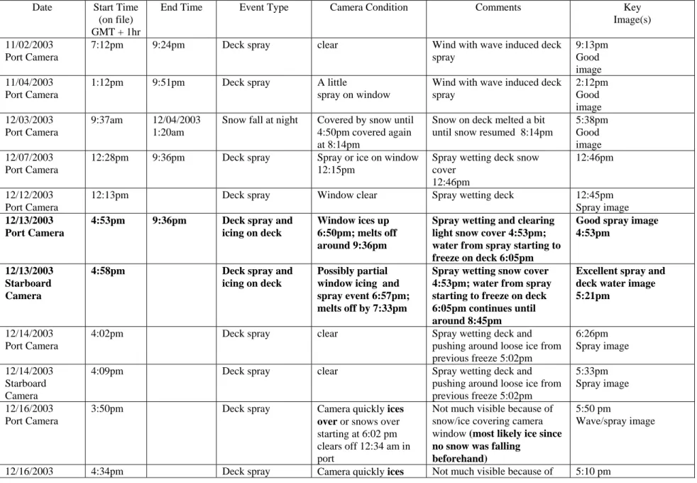
LIST OF TABLES Table 1: Summary of MIMS observations during winter of 2003/2004………..…….6
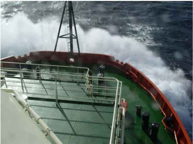
LIST OF FIGURES Figure 1: Large splash against Kingfisher hull……….8
Figure 2: Spray from wave-hull interaction (Kingfisher)………..………8
Figure 3: Monitoring system’s general components and configuration…...………… 9
Figure 4: Port and starboard camera locations………...……….9
Figure 5: Plot of ice thickness versus time for an icing event……….………….10
Figure 6: Base image used for comparison (no ice)………..…………10
Figure 7: Original image (with ice) and grayscale copy of it………...….11
Figure 8: Rotated image and zoomed to area of interest………….………11
Figure 9: Initial and refined edge detections……….……….11
Figure 10: Overlay of edge detection and close up……….………12
Figure 11: Popup window displaying ice thickness……….12
APPENDICES
Appendix A: Matlab Code for Kingfisher Ice Thickness Data (Single Image) Appendix B: Matlab Code for Manual Measurement of Distance
AUTOMATED ANALYSIS OF MARINE ICING IMAGES 1.0 INTRODUCTION
This report will focus on the Marine Icing Monitoring System (MIMS) and what it is used for. As more and more vessels and structures are set out to sea we run into more and more risks and challenges to keep these vessels safe. Marine spray icing is very common and can be quite dangerous if not carefully watched. The Institute for Ocean Technology (IOT) has developed MIMS to counteract and study marine spray icing.
2.0 MARINE SPRAY ICING
Marine spray icing occurs when certain weather conditions arise. Basically, it is when water crashes into the hull of a ship and creates a large upward splash. If there is significant wind the splash may get blown over the ship as a spray. And finally, if it is cold outside, you can expect that spray to freeze onto the ship. (See Figures 1 and 2) Heavy ice buildup can lead to the increased size and weight of the vessel, increase the draught of a vessel, and change the centre of vessel gravity. Simply put, icing
influences its stability, and can potentially cause a vessel to capsize or sink.
2.1 Influencing Factors
The main factors influencing marine spray icing are: Wind speed; Wave height; and Temperature. Vessel Icing occurs in wind speeds of about 9 m/s (sometimes lower), Temperature of approximately -2 °C and wave heights as low as 1m. Basically, if the temperature gets below -2 °C and there is a little wind, be prepared for icing to occur.
2.2 Preventative Measures
The best way to prevent getting caught in an icing event would be to stay at the dock if an icing storm is forecast, but that is not feasible for some seafarers. There are various coatings available to be applied to the superstructure of vessels. Some will act like a wax and get water to “bead” off of the surfaces. Others will allow for easier removal of ice, once it has already frozen on to the structure. In any case, there should always be a few sledgehammers and axes on board for removal of ice if you are entering water susceptible to these events.
3.0 MONITORING SYSTEM
The Marine Icing Monitoring System (MIMS) is a visual based technology for monitoring marine ice accumulation on offshore rigs and vessels where icing poses operational and safety hazards. (Gagnon, R. September 2004) The system is completely stand-alone, requiring no maintenance, needing only a standard 110 VAC power supply, and draws approximately 300 Watts. MIMS was first installed on the Caribou and is now actively collecting data on board the Kingfisher.
3.1 Components
The system consists of a CPU connected to two high resolution digital cameras that are positioned to view expansive areas, or smaller areas depending on requirements, where icing could occur when environmental conditions are within certain parameters. Multiple units could be used to cover more sites on the vessel. (See Figures 3 and 4)
When turned on, the computer controls each camera and causes the cameras to take pictures at regular intervals (every 12 minutes) that are downloaded
immediately to the computer’s hard drive. Data is retrieved from the hard drive at the end of the icing season.
The system has a satellite phone so that it can be controlled from IOT.
Thumbnail images can be quickly downloaded to monitor current conditions at the site, and the cameras can be controlled to zoom in or out. Full size images may also be downloaded; however, several minutes are required to download one image, whereas thumbnail images can be retrieved in a matter of a few seconds.
3.2 Ruggedization
Modifications and extensive ruggedization were carried out at IOT on the
originally purchased cameras. They were equipped with metal casings that have a Plexiglas window in the front. The casings then had to be well insulated to keep the electronics safe from the winter elements. Heaters we installed inside the casings to keep the window from freezing and to keep the camera functioning correctly. It was found out that the window would still sometimes freeze when spray would get in contact with it and would take some time to thaw. Because of this addition heater were added directly to the window itself. Also, the originally used satellite phone was not reliable and has since been replaced by a much better system that has seen no problems thus far.
4.0 IMAGE PROCESSING
The images captured by MIMS are collected at the end of the winter season and are then analyzed. Data such as sea state, ice thickness, weather conditions, time, and type of event are all noted. (See Table 1) Matlab is used for “Smart”, automated analysis. Information such as ice thickness, average thickness, and rate of buildup can be calculated using this method. It is very accurate and requires only a slight tuning from the general code (See Appendix A) to work with any other structure. The current script will only work for the Kingfisher application. I have also developed a more manual method of measurement for digital images, using Matlab, to check the automated results. (See Appendix B)
4.1 Techniques
There are many image processing techniques used depending on the situation. Some may be excellent for one image but give mediocre results on other images. The key is trying all possible methods and choosing the one that will work out the best on the majority of the images. If it is possible to use simple functions then do so, try not to overcomplicate things. It is impossible to determine the thickness of ice at every possible spot on a structure and a limited time, so focus on discrete logical areas to take your measurements from.
The most important thing to do is to first convert the image into grayscale. This brings every color into a relationship on a single scale, black being one, white being zero and everything else somewhere in between. The next thing to do when you are only interested in one area of an image is to remove the remaining part. To do this, create a binary mask. For example, in the area of interest
choose values of 1 and zeros for the rest. Then multiply this with the image you want to process. It will leave you with only the important part, which makes the computers job much simpler when it comes to the later processing and easier for you to see what’s going on as well.
Edge detection is one of the simpler image processing techniques and at the same time one of the most powerful. Basically, they look at one pixel, then the next and try to determine if there is a large change in the intensity of your
grayscale image. If there is a large gradient found then that will be considered an edge. This is not always correct for many reasons, but you can do a second edge detection with a different gradient threshold and remove what was once thought to be an edge, or vice versa. Most edge detection techniques (there are a lot) work best when they are finding either a vertical or horizontal line. For this
reason, if possible, rotate the image so that the edge you are looking for is in the vertical or horizontal position.
There are hundreds of other functions and methods of fixing certain problems with images. They are best understood through actually trying them out to see what results you get. If it’s not what you wanted try something different.
Eventually you get a fell for what will happen when you apply a certain filter and can make quick work of a complex image with the use of simple functions.
4.2 Execution
For this particular application on the Kingfisher there have been two methods developed for processing the captured images. The first method deals with processing a single image, but gives a visual representation of every step by displaying the new image after every function has been performed. The second method does the same analysis as the single image one, but does not show an image for every intermediate step. Instead it processes an entire icing event (~25 images or 5 hrs) and puts the results into an Excel spreadsheet for easy viewing. It also displays a plot of the ice thickness versus time with a trend line to take account of outliers that did not get processed properly. (See Figure 5) As said
before, some images do not get processed properly. This is due to water or ice on the camera or a wave splashing when the image was captured and is
unavoidable.
4.2.1 Single image Processing
See Appendix A for Matlab code and Figures 6 to 11 correspond to the bullets below. Here is a breakdown of what the code is actually doing. After each step it displays the image for you to see.
• Load the mask for the area of interest then read and display image • Convert it to grayscale and rotate so the structure is vertical
• Remove the remainder of the image we are not interested in • Initial edge detection to get the automatically calculated threshold • Change the threshold and do a refined edge detection to remove
image noise and unwanted edges
• Take the refined edge detection and rotate it back, then overlay it onto the original image to check for accuracy
• Search for the left and right edges of the ice and determine the total width of the ice covered pole
• From that, determine the thickness of ice and display a popup window showing the value
4.2.2 Sequence of images
See Appendix C for Matlab code and Figure 5 for the output Excel plot. Below is a breakdown of the Matlab code in Appendix C.
• Load the area mask and the sequence of images to be used • Perform a loop and do the Single image analysis on each image • Create an array to hold all of the data for each image
• Calculate the average thickness of ice
• Retrieve the header information from excel to determine where to place your current data
• Write the data to an excel spreadsheet with each individual thickness and the average thickness of ice during the event
4.3 Improvements
This technology is by no means perfect and there is always room for
improvement. Below is a list of a few things that could be improved as this project continues.
• There has been only enough time to study one particular area of a structure, for a more complete analysis multiple areas should be used to collect data.
• Only a vertical member has been studied, the horizontal members act quite differently and may need to take a different approach when analyzing them. Ice buildup is not as uniform as a vertical member.
• Only the starboard camera is being used to collect the ice thickness data, I similar script could be written and implemented for the port side camera to give a denser timeline of events.
• More work put into images that are difficult to analyze (spray or water partially covering structure) so they can also be used to retrieve data from. • Optimization of some of the loops and functions may be possible to speed
Table 1. Summary of MIMS observations during winter of 2003/2004 deployment on Caribou ferry
Date Start Time End Time (on file)
GMT + 1hr
Event Type Camera Condition Comments Key Image(s) 11/02/2003
Port Camera
7:12pm 9:24pm Deck spray clear Wind with wave induced deck spray 9:13pm Good image 11/04/2003 Port Camera
1:12pm 9:51pm Deck spray A little
spray on window
Wind with wave induced deck spray 2:12pm Good image 12/03/2003 Port Camera 9:37am 12/04/2003 1:20am
Snow fall at night Covered by snow until 4:50pm covered again at 8:14pm
Snow on deck melted a bit until snow resumed 8:14pm
5:38pm Good image 12/07/2003
Port Camera
12:28pm 9:36pm Deck spray Spray or ice on window 12:15pm
Spray wetting deck snow cover
12:46pm
12:46pm
12/12/2003 Port Camera
12:13pm Deck spray Window clear Spray wetting deck 12:45pm Spray image
12/13/2003 Port Camera
4:53pm 9:36pm Deck spray and icing on deck
Window ices up 6:50pm; melts off around 9:36pm
Spray wetting and clearing light snow cover 4:53pm; water from spray starting to freeze on deck 6:05pm
Good spray image 4:53pm
12/13/2003 Starboard Camera
4:58pm Deck spray and icing on deck
Possibly partial window icing and spray event 6:57pm; melts off by 7:33pm
Spray wetting snow cover 4:53pm; water from spray starting to freeze on deck 6:05pm continues until around 8:45pm
Excellent spray and deck water image 5:21pm
12/14/2003 Port Camera
4:02pm Deck spray clear Spray wetting deck and pushing around loose ice from previous freeze 5:02pm 6:26pm Spray image 12/14/2003 Starboard Camera
4:09pm Deck spray clear Spray wetting deck and pushing around loose ice from previous freeze 5:02pm
5:33pm Spray image 12/16/2003
Port Camera
3:50pm Deck spray Camera quickly ices
over or snows over
starting at 6:02 pm clears off 12:34 am in port
Not much visible because of snow/ice covering camera window (most likely ice since
no snow was falling beforehand)
5:50 pm
Wave/spray image
Starboard Camera
over or snows over
starting at 5:58 pm clears off 10:38 pm in port
snow/ice covering camera window (most likely ice since
no snow was falling beforehand) Wave/spray image 12/22/2003 Starboard Camera 5:46pm Apparent small amount of ice on deck
clear Icing from apparent refreezing snow cover melt. No apparent deck spray
5:46 pm Deck ice 01/01/2004
Port Camera
4:12pm 7:36pm Deck spray wetting snow cover
Camera gets some spray and possible ice (partial cover) around 4:48pm clears off at 7:36pm
Not sure if wetted snow on deck ices up after wetting
5:48 pm
Window obscured a little, wind and spray visible, deck in process of wetting
01/05/2004 Port Camera
4:53pm 7:18pm Deck spray and icing on deck
Mostly clear Spray wetting deck 4:53pm; water from spray starting to freeze on deck 5:06pm continues until around 7:18pm
Excellent spray and accumulated deck ice image 6:06pm 01/07/2004 Starboard Camera 4:06pm Deck spray wetting previous and newly falling snow yielding frozen wetted snow on deck
Window ices over from spray and snow at 5:06pm and melts off in port at 2:18am
Spray wetting snow cover mixed with freshly falling snow starting around 4:06pm
Good image of freezing wetted snow on deck and starting on camera window 4:42pm 01/09/2004 Starboard Camera 4:12pm Deck spray wetting snow cover with previous frozen wetted snow underneath
Window ices over from spray at 4:24pm and melts off by 7:50pm
Good image spray wetting snow and ice on deck and some icing on camera window 5:48pm 01/17/2004 Starboard Camera 3:12pm Spray in air wetting deck
Clear usually, but a few images show spray on window (probably liquid)
Other images show sloshing deck water from spray 3:42pm, 3:54pm, 4:06pm
Excellent image of generated spray in air impinging on deck 3:12pm
01/20/2004 Starboard/Port Cameras
4:42pm Ice on window Window icing starting at 4:42pm and clears around 9:49pm 01/23/2004 Starboard Camera 5:42pm Snow/ice on window
Window snows over, probably turning to ice, starting at 5:42pm and doesn’t clear off until Jan. 25 at 3:30pm
Figure 1. Large splash against Kingfisher hull
Figure 3. Monitoring system’s general components and configuration
Ice Thickness vs Time 0 0.5 1 1.5 2 2.5 3 3.5 4 4.5 1 2 3 4 5 6 7 8 9 10 11 12 13 14 15 16 17 18 19 20 21 22 Time (min x 12) Ic e T h ick n e ss (c m ) Kingfisher data Trendline
Figure 5. Plot of ice thickness versus time for an icing event.
Figure 7. Original image (with ice) and grayscale copy of it
Figure 8. Rotated image and zoomed to area of interest
Figure 10. Overlay of edge detection and close up
Appendix A
Matlab Code for Kingfisher Ice Thickness Data Retrieval
% clear current workspace and load the correct one clear variables; load('bar_masks.mat') % read in images I1 = imread('D291900F.jpg');
cd('E:\Test Image sequence');
% show original image
figure, imshow(I1); title('Original Image'); imwrite(I1,'I1.bmp','bmp'); % convert to grayscale BW1 = rgb2gray(I1); figure, imshow(BW1); title('Grayscale'); imwrite(BW1,'BW1.bmp','bmp'); % rotate image
BW1 = imrotate(BW1,-9.5,'bilinear','crop'); figure, imshow(BW1);
title('Rotated');
imwrite(BW1,'Rotated.bmp','bmp');
% remove remainder of image
cutout = immultiply(mask1,BW1); figure, imshow(cutout); title('Cutout'); imwrite(cutout,'Cutout.bmp','bmp'); % edge detection
[ed,At] = edge(cutout,'sobel',[],'both','thinning'); figure, imshow(ed);
title('Initial Edge Detection'); imwrite(ed,'InitialED.bmp','bmp');
% Change the automatically computed thresholds
k = 8;
ed = edge(cutout,'sobel',k*At,'both','thinning'); ed = bwmorph(ed,'clean');
figure, imshow(ed)
title('Refined Edge Detection'); imwrite(ed,'RefinedED.bmp','bmp');
% overlay onto the original image
ed_rot = zeros(1712,2288,3); for r = 1:1712 for c = 1:2288 for k = 1:3 if ed(r,c) == 1 ed_rot(r,c,k) = 1; end; end; end; end;
ed_rot = imrotate(ed_rot,9.5,'bilinear','crop'); orig_overlay = I1;
for r = 1:1712 for c = 1:2288 for k = 1:3
A-1 end; end; end; end; figure, imshow(orig_overlay); title('Edge Detection Overlay');
imwrite(orig_overlay,'EDOverlay.bmp','bmp');
cd('M:\My Documents\MatLab');
% search for left and right boundaries
y = 540; x1 = 976; x2 = 987; while ed(y,x1) == 0 x1 = x1-1; end; while ed(y,x2) == 0 x2 = x2+1; end; %x1 %x2
% determine the thickness of ice
cmperpixel = 0.5; pole = 17;
width = x2 - x1 + 1;
thickness = cmperpixel*(width - pole)/2;
% calculate average thickness for the sequence
total_thick = total_thick + thickness; avg = total_thick;
ave_thick = ['Avg: ' num2str(avg)];
% put values in data array for export to excel
outdata{3,1} = thickness;
%display result
message = ['Ice thickness of: ' num2str(thickness) ' cm']; msgbox(message,'Ice Measurement','help');
A-2
Appendix B
Matlab Code for Manual Measurement of Distance
% Algorithm to make a measuring tool appear over an image
% Choose the image
[filename,pathname] = uigetfile({'*.jpg';'*gif';...
'*.tif';'*.png'},...
'Select Image'); cd(pathname);
hImg = imshow(filename);
% Convert XData and YData to meters using conversion factor.
cmetersPerPixel = 1/4;
XDataInCMeters = get(hImg,'XData')*cmetersPerPixel; YDataInCMeters = get(hImg,'YData')*cmetersPerPixel;
% Set XData and YData of image to reflect desired units.
set(hImg,'XData',XDataInCMeters,'YData',YDataInCMeters); set(gca,'XLim',XDataInCMeters,'YLim',YDataInCMeters);
% Specify position of distance tool in terms of XData/YData units.
hline = imdistline(gca,[150 250],[100 100]); api = iptgetapi(hline);
Appendix C
Matlab Code for Kingfisher Ice Thickness Data (Image Sequence)
% and export the data to a Microsoft excel spreadsheet
% clear current workspace and load the proper one
clear variables; load('bar_masks.mat')
% read in images
cd('E:\Test Image sequence');
load('image_sequence.mat')
cd('M:\My Documents\MatLab');
% Loop through several images for i = 1:36 I1 = I{1,i}(:,:,:); % convert to grayscale BW1 = rgb2gray(I1); % rotate image
BW1 = imrotate(BW1,-9.5,'bilinear','crop');
% remove remainder of image
cutout = immultiply(mask1,BW1);
% edge detection
[ed,At] = edge(cutout,'sobel',[],'both','thinning');
% Change the automatically computed thresholds
k = 8;
ed = edge(cutout,'sobel',k*At,'both','thinning'); ed = bwmorph(ed,'clean');
% overlay onto the original image
ed_rot = zeros(1712,2288,3); for r = 1:1712 for c = 1:2288 for k = 1:3 if ed(r,c) == 1 ed_rot(r,c,k) = 1; end; end; end; end;
ed_rot = imrotate(ed_rot,9.5,'bilinear','crop'); orig_overlay = I1; for r = 1:1712 for c = 1:2288 for k = 1:3 if ed_rot(r,c,k) ~= 0 orig_overlay(r,c,k) = 1; end; end; end; end;
% search for left and right boundaries
y = 540; x1 = 976; x2 = 987; while ed(y,x1) == 0 x1 = x1-1; end;
C-1 x2 = x2+1;
end;
% determine the thickness of ice
cmperpixel = 0.5; pole = 17;
width = x2 - x1 + 1;
thickness = cmperpixel*(width - pole)/2;
%calculate average thickness for the sequence
total_thick = total_thick + thickness; avg = total_thick/i;
ave_thick = ['Avg: ' num2str(avg)];
% put values in data array for export to excel
outdata{i+2,1} = thickness;
end;
% get date and use as header for next excel column
[indata, inheader] = xlsread('Marine_Icing_Thickness.xls', 'Kingfisher'); siz = size(inheader); j = siz(1,2) + 1; outdata{1,1} = date; outdata{2,1} = ave_thick; column = [convert{j} '1'];
% write data to excel spreadsheet
xlswrite('Marine_Icing_Thickness.xls', outdata, 'Kingfisher', column);