Coherent decay of Bose-Einstein condensates

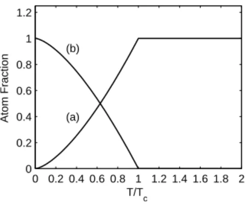
We start by introducing the thermodynamics of Bose gases near the critical temperature for Bose-Einstein condensation, and what are the expected deviations to the ideal gas picture

Finally we review results obtained with a quadratic + quartic potential, which allows to study a regime where the rotation frequency is equal to or larger than the harmonic

We describe how the QZ effect turns a fragmented spin state, with large fluctuations of the Zeeman populations, into a regular polar condensate, where the atoms all condense in the m

Our theoreti- cal calculations show that, by transferring the atoms into a shallow trap, the spin squeezed states created in [40] can survive more than 0.5 second under the influence

Les deux types d’antiseptiques ont leur place dans notre monde, les antiseptiques de synthèse étaient toujours efficaces puisqu’ils sont plus commercialisés et

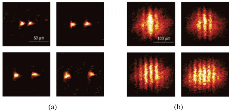
By looking at the number of scattered atoms in the x direction (perpendicular to the plane of Fig. 2), we have verified that, away from the endfire modes, the rate of emission varies

We show in particular that in this strongly degenerate limit the shape of the spatial correlation function is insensitive to the transverse regime of confinement, pointing out to

In this Letter, we propose an analogue of the RFIO effect using two BECs trapped in harmonic potentials and coupled via a real-valued random Raman field.. We show that the