Control, gates, and error suppression with Hamiltonians in quantum computation

(1)

Control, Gates, and Error Suppression with Hamiltonians

in Quantum Computation

by

Adam Darryl Bookatz

Submitted to the Department of Physics

in partial fulfillment of the requirements for the degree of

Doctor of Philosophy in Physics

at the

MASSACHUSETTS INSTITUTE OF TECHNOLOGY

MASSACHUSETTS INSTITUTE OF TECHNOLOGY

JUN

09 2016

LIBRARIES

June 2016

@ Massachusetts Institute of Technology 2016. All rights reserved.

Author ...

Certified by...

Accepted by ...

Signature redacted

Department of Physics

May 12, 2016

Signature redacted

_{. ... ...}

_....

_...

Edward Farhi

Cecil and Ida Green Professor of Physics;

Director, Center for Theoretical Physics

Thesis Supervisor

Signature redacted

Nergis Mavalvala

Curtis and Kathleen Marble Professor of Astrophysics

Associate Department Head for Education, Physics

(2)

(3)

Control, Gates, and Error Suppression with Hamiltonians in Quantum Computation

by

Adam Darryl Bookatz

Submitted to the Department of Physics on May 12, 2016, in partial fulfillment of the

requirements for the degree of Doctor of Philosophy in Physics

Abstract

In this thesis we are primarily interested in studying how to suppress errors, perform sim-ulation, and implement logic gates in quantum computation within the context of using Hamiltonian controls. We also study the complexity class QMA-complete.

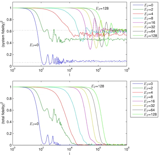
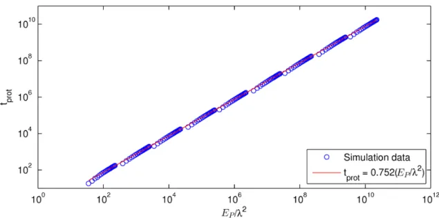
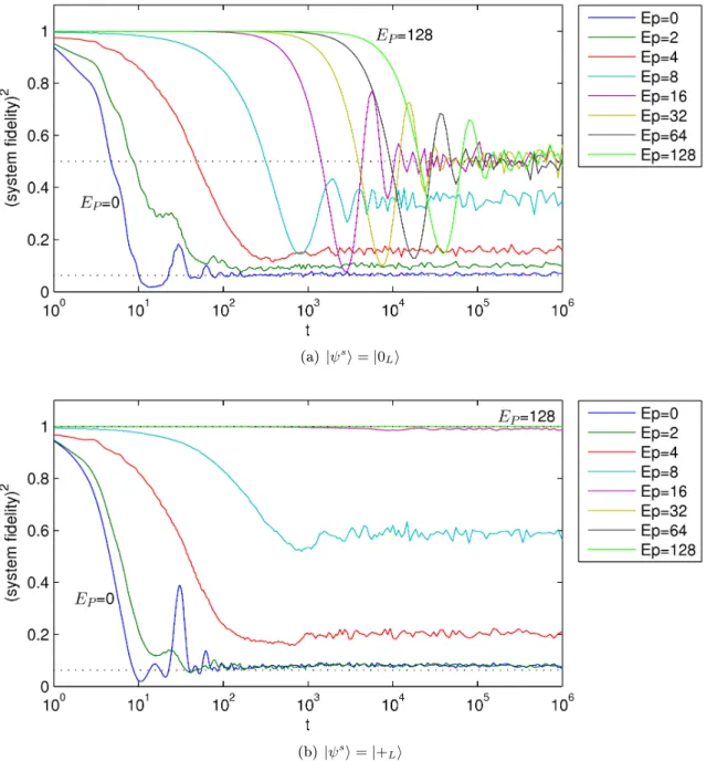
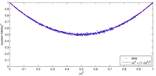
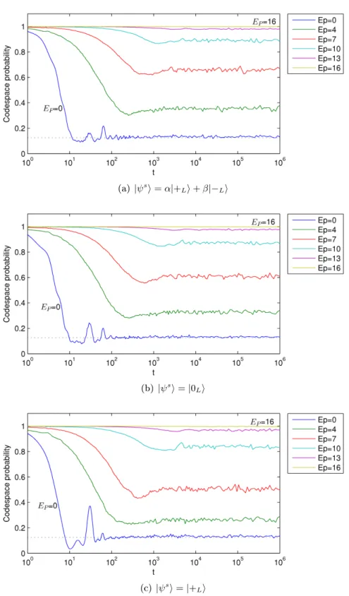
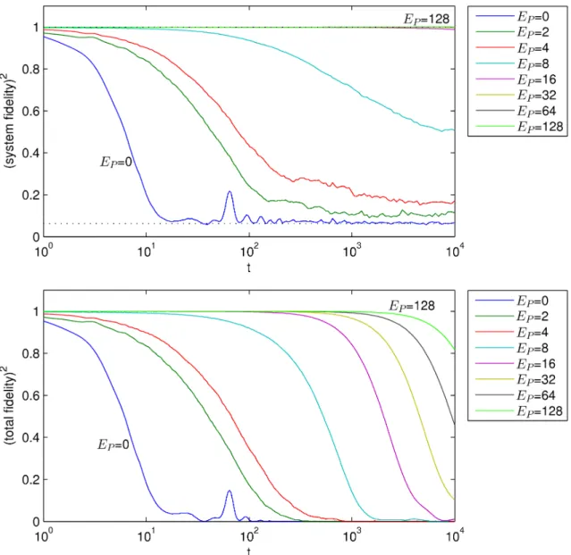
We first investigate a method (introduced by Jordan, Farhi, and Shor) for suppress-ing environmentally induced errors in Hamiltonian-based quantum computation, involvsuppress-ing encoding the system with a quantum error-detecting code and enforcing energy penalties against leaving the codespace. We prove that this method does work in principle: in the limit of infinitely large penalties, local errors are completely suppressed. We further derive bounds for the finite-penalty case and present numerical simulations suggesting that the method achieves even greater protection than these bounds indicate.

We next consider the task of Hamiltonian simulation, i.e. effectively changing a sys-tem Hamiltonian to some other desired Hamiltonian by applying external time-dependent controls. We propose protocols for this task that rely solely on realistic bounded-strength control Hamiltonians. For systems coupled to an uncontrollable environment, our approach may be used to perform simulation while simultaneously suppressing unwanted decoherence. We also consider the scenario of removing unwanted couplings in many-body quantum systems obeying local system Hamiltonians and local environmental interactions. We present protocols for efficiently switching off the Hamiltonian of a system, i.e. simulating the zero Hamiltonian, using bounded-strength controls. To this end, we introduce the combinatorial concept of balanced-cycle orthogonal arrays, show how to construct them from classical error-correcting codes, and show how to use them to decouple 𝑛-qudit ℓ-local Hamiltonians using protocols of length at most 𝑂(𝑛ℓ−1_{log 𝑛).}

We then present a scheme for implementing high-fidelity quantum gates using a few interacting bosons obeying a Bose-Hubbard Hamiltonian on a line. We find high-fidelity logic operations for a gate set (including the cnot gate) that is universal for quantum information processing.

Lastly, we discuss the quantum complexity class QMA-complete, surveying all known such problems, and we introduce the “quantum non-expander” problem, proving that it is QMA-complete. A quantum expander is a type of rapidly-mixing quantum channel; we show that estimating its mixing time is a co-QMA-complete problem.

Thesis Supervisor: Edward Farhi

(4)

(5)

Acknowledgements

First and foremost, I would like to thank my wife, Josepha, for her steadfast support and encouragement and for cheerfully putting up with having a graduate student for a husband. I am especially grateful to my advisor, Eddie Farhi, for being a great thesis supervisor, giving me both direction and freedom, as well as exemplifying how to write academic papers with precision and clarity. I also especially thank Pawel Wocjan, for being like a second advisor to me, sharing much wisdom – in science, career, and life – and working on many projects with me. In addition, I greatly appreciate the help of all of my collaborators, Yoav Lahini, Martin Roetteler, Leo Zhou, Greg Steinbrecher, Stephen Jordan, Yi-Kai Liu, Lorenza Viola, and Dirk Englund. Thank you to my thesis committee members, Edward Farhi, Aram Harrow, and Boleslaw Wyslouch for carefully reading and checking my thesis, thereby comforting me that at least someone has read it.

I feel privileged to have been able to attend MIT, with its strong series of quantum information courses, and I thank my teachers, Professors Isaac Chuang, Scott Aaronson, and Peter Shor for their classes from which I benefited greatly. The help, advice, and discussions with MIT postdocs and students has also been invaluable, and I want to thank Shelby Kimmel, Cedric Lin, Han-Hsuan Lin, David Gosset, Lior Eldar, Kristen Temme, Iman Marvian, as well as professors Barton Zwiebach, Aram Harrow, Seth Lloyd, and Sam Gutmann. I thank the many people of the faculty and staff of the CTP, the Department of Physics, and MIT who have helped me and taught me, and I also thank the MIT Rowing Club for helping me ward off physical atrophy long enough to write this thesis.

Lastly, I thank my parents, Brian and Sandra, for their continuous support throughout my entire life, and my brothers, David and Gidon, for being great brothers and keeping me suitably distracted when appropriate; I am truly fortunate to have such a family.

(6)

(7)

Chapter 0 Thesis introduction

Quantum computing proposes the exciting possibility of exploiting the ‘weirdness’ of quan-tum mechanics to develop a new paradigm of computing. While quanquan-tum computers are widely believed to be more powerful than classical computers for certain important tasks (such as factoring and unstructured searches), the question of what computational power practical quantum computation yields remains open. Moreover, it appears that the tech-nology of scalable quantum computers is still beyond the near-future, so studying how to overcome the obstacles that impede building even small-scale quantum computers is a crucial topic to the field. This thesis addresses, in part, both of these questions.

In classical computing, by which we mean regular, non-quantum computing, the basic unit of information is the bit – an object that can be in precisely one of two states, 0 or 1. If we have 𝑛 bits, each of them is either 0 or 1, so a system of 𝑛 bits can always be specified by 𝑛 parameters – one simply records the value of each bit. Note that there are 2𝑛_possible

𝑛-bit values. The quantum setting is much richer. And, to the best of our knowledge, it is also fundamentally how our world really operates. Quantum mechanics allows for two-state objects (e.g. an electron’s spin), so like a bit, such a system can be 0 or 1. But unlike a bit, the quantum state need not be only 0 or 1; it can be in a superposition of both 0 and 1 “at the same time”. Such a quantum bit is called a qubit. However, the fundamental difference between classical and quantum computing is seen not from a single qubit but from many qubits. For with 𝑛 qubits, each of the 2𝑛_{possible 𝑛-bit values are now merely the basis states}

allowed in the superposition. Specifying a system of 𝑛 qubits involves, in general, keeping track of all 2𝑛_{coefficients of each of those basis states, i.e. “how much” of the state is in each}

of the 2𝑛 _𝑛_{-bit values. This is not to say that quantum computers can yield exponentially}

more information than classical computers. The information contained in these coefficients is not immediately accessible. To obtain information from the state, one must measure it, and when one measures a quantum state, the superposition collapses, giving just one of the 2𝑛 _{classical bit strings. Indeed, someone with a background in stochastic (random)}

processes may not think this quantum picture, as described so far, sounds particularly powerful – one may think these coefficients represent mere probabilities, making a collection of 𝑛 qubits no different from a probabilistic mixture of 𝑛 bits. But unlike probabilities, these coefficients are not non-negative numbers; they can be negative (or even complex), so that when processing quantum information, components of the superposition may undergo complicated cancellations (interference) that cannot occur with random bits.

If this sounds complicated, it is because it is. We still have a long way to go in under-standing how to harness the power of the quantum world for use in computation. Much

(12)

progress has been made in the past three decades. Of particular interest are two algorithms – Grover’s algorithm and Shor’s algorithm – that have attracted a lot of attention to the field of quantum computing. Grover’s algorithm allows a quantum computer to search for a marked item amongst 𝑁 items, taking only time proportional to √𝑁 to do so (as opposed to the classical scenario, where such a search could require looking at all 𝑁 items and there-fore takes time proportional to 𝑁). Shor’s algorithm allows a quantum computer to factor integers (15 = 5 × 3 being a very simple example). This problem is believed to be difficult for regular computers – one can factor 15 = 5 × 3 in their head, but even with a modern supercomputer, factoring a 400-digit number seems to be extremely difficult. In fact, our confidence in the difficulty of this problem has led to it being widely used in cryptography: currently, sending sensitive information (like your credit card) over the internet relies on techniques like RSA encryption to keep it secret, and the security of RSA relies solely on the difficulty of factoring large numbers. Shor’s algorithm shows that a quantum computer could factor integers efficiently and break RSA encryption easily.

Although there is much interest in the field of quantum computing, the goal of ac-tually building a large-scale quantum computer currently remains beyond reach. One of the greatest obstacles to accomplishing this goal is overcoming errors due to environmental disturbance. A quantum system with unwanted interactions from an uncontrollable envi-ronment will decohere, i.e. lose much of the extra quantum information held within the superposition states. Practically, attempting to isolate the system from the environment has limitations – after all, the device is meant to be a computer, necessitating control and measurement via external interaction. A major push in the field of quantum computing has therefore been towards suppressing and correcting errors arising during computation, and much progress has been made, at least theoretically. Indeed, in the most common model of quantum computing – the circuit model – it has been shown that, provided error rates are below some constant value, arbitrarily-accurate quantum computation can, in principle, be performed efficiently.

The circuit model describes quantum computation in terms of instantaneous operations (gates), similar to the notion of logical and, or, not, and nand gates in classical circuits. It is not, however, the only model of quantum computation. It is also somewhat of an idealization, as it treats these gates as being implemented instantaneously without dealing with the underlying physical machinery performing the operations. In quantum physics, systems are generally described by Hamiltonians – operators defining the energy of the system and responsible, via the Schrödinger equation, for their evolution. There are a number of models of quantum computation described in terms of Hamiltonians, including the original vision of quantum computation by Richard Feynman, who is often credited with pioneering the field, as well as the model of adiabatic quantum computation, upon which the widely-publicized (but non-universal) D-Wave architecture is based. Such models, which we term Hamiltonian-based quantum computation in this thesis, involve specifying the Hamiltonian of a system, evolving the system in time under this Hamiltonian (with no intermediate measurements or instantaneous operations allowed), and performing a final measurement. We will primarily focus on such a setting in this thesis, where systems, and our control over them, are restricted to (non-instantaneous) Hamiltonian evolution. Within this context:

∙ we analyse an error suppression technique for Hamiltonian-based quantum computa-tion, proving that it works in principle;

(13)

system-environment couplings;

∙ we develop protocols for Hamiltonian simulation (i.e. having a system defined by one Hamiltonian behave as though it were defined by a different Hamiltonian), again suppressing unwanted environmental disturbance; and

∙ we develop realizable or near-future-realizable Hamiltonians for implementing useful quantum gates.

Another topic of interest when studying Hamiltonian models of quantum computing is what computational power they provide. Historically, there has been a strong connection between this question (at least for adiabatic quantum computing) and the study of the quantum complexity class called QMA-complete. In this thesis,

∙ we discuss what problems are known to be in this class and

∙ we prove that it contains a particular problem involving so-called quantum expanders, which are, among other things, related to the thermalization of quantum systems coupled to an environment.

In the next section, we elaborate on these points, outlining the content that comprises this thesis.

0.1 Outline

Each chapter in this thesis is self-contained, with its own bibliography and appendices (if applicable) at the end of the chapter. First, in Chapter 1, we provide much of the back-ground required for the remainder of the thesis, presenting a broad overview of the topics needed to understand the later material. More technical background will be introduced in the individual chapters as needed, as will references for further study. We now outline the contents of these chapters (with references to the applicable background sections given in parentheses).

As noted, a challenging obstacle towards building quantum computers is protecting them from unwanted environmental disturbance. In the usual circuit model of quantum computa-tion (Sec. 1.3), the theory of quantum error correccomputa-tion has been well-developed, suggesting that, in principle, quantum computation can be performed in a manner resistant to such environmental disturbance; however, the question of how well Hamiltonian-based quantum computation models (Sec. 1.2) can be protected from error remains open. One proposal (introduced by Jordan, Farhi, and Shor) for suppressing environmentally induced errors in Hamiltonian-based quantum computation is the use of quantum error-detecting codes (Sec. 1.5.2), together with energy penalties against leaving the codespace. In Chapter 2 we prove that this method does work in principle: in the limit of infinitely large penalties, errors are completely suppressed. We also derive bounds for the finite-penalty case and perform numerical simulations that suggest that the energy penalty method achieves even greater protection than these bounds guarantee.

Related to the goal of the previous paragraph are Hamiltonian decoupling and Hamilto-nian simulation, in the context of quantum control theory. In HamiltoHamilto-nian decoupling, one seeks to switch off the Hamiltonian of a system, removing unwanted internal and system-environment couplings (the latter being responsible for decoherence errors). More generally, in Hamiltonian simulation one is interested in removing these unwanted couplings while

(14)

simultaneously effectively changing the system Hamiltonian to simulate a different, desired Hamiltonian. These tasks would be useful, for example, for quantum memories and analogue quantum simulators (Sec. 1.2.4), respectively, while addressing the ever-important objective of suppressing environmental errors. In contrast to many previous protocols for these tasks that rely on using instantaneous unitary pulses (which, in terms of Hamiltonians, require controls of unbounded strength, and are therefore fundamentally unphysical), we are inter-ested in the setting in which all controls can be described using bounded-strength Hamil-tonians. In Chapter 3 we develop a control protocol for Hamiltonian simulation that uses only bounded-strength controls by combining a Hamiltonian simulation scheme that uses controls of unbounded-strength, with a bounded-strength decoupling scheme called Eulerian decoupling.

Another issue for general-purpose decoupling and simulation protocols is that they are often inefficient, requiring very long control sequences. By making physically-reasonable assumptions about the quantum system of interest, however, we can hope to devise better protocols. In Chapter 4 we develop efficient bounded-strength decoupling protocols for local Hamiltonians, i.e. for quantum systems in which each qubit interacts with only a few other qubits, as is typically the case in nature (Sec. 1.1.4). To do so, we introduce the combinatorial concept of balanced-cycle orthogonal arrays, demonstrate how to construct them from classical error-correcting codes (Sec. 1.5.1), and show how to exploit the locality of the system with them to perform decoupling more efficiently.

While the previous topics address Hamiltonian-based quantum computation and Hamil-tonian simulation, the most common model of quantum computation is the circuit model (Sec. 1.3), in which computation is described by a sequence of unitary operations (gates). As noted, this model is somewhat of an idealization, ignoring the question of how these uni-tary operations are to be performed. Nonetheless, in a real physical system actualizing this computation, each step is generally performed by implementing some corresponding Hamil-tonian. Designing a physically-realizable Hamiltonian to implement a desired unitary gate, while obeying the constraints of the physical platform available, is in general a non-trivial problem. Inspired by continuous-time quantum walks (Sec. 1.2.3), in Chapter 5 we present a method for implementing high-fidelity quantum logic gates using interacting bosons on a one-dimensional lattice (Sec. 1.1.6). Specifically, constraining ourselves to experimentally feasible system parameters, we present high-fidelity logic operations for a gate set, including the cnot gate (Sec. 1.3.2), that is universal for quantum information processing.

Aside from the important question of how to practically implement quantum computa-tion, another important question is what computational power the quantum setting provides. This question is addressed by the field of quantum complexity theory (Sec. 1.4.2). In this thesis, we are primarily interested in the quantum complexity class known as QMA-complete, the quantum analogue of the classical class NP-complete. Informally, QMA-complete con-sists of the problems whose solutions are believed to be hard to find – but easy to verify – using a quantum computer. The development of the QMA-complete class and its most fa-mous member, the local Hamiltonian problem (Sec. 1.4.3), has been highly connected to analysing the power of using local Hamiltonians for Hamiltonian-based computation meth-ods, notably that of adiabatic quantum computation (Sec. 1.2.1). A survey of all known QMA-complete problems is the content of Chapter 7.

Adding to the list of known QMA-complete problems, in Chapter 6 we classify the complexity of the quantum non-expander problem as being QMA-complete. Quantum expanders are the quantum analogues of expander graphs (which play a prominent role in computer science and discrete mathematics), and are related to the thermalization of open

(15)

quantum systems. They are quantum operations (Sec. 1.1.5) that rapidly take quantum states towards the maximally mixed state (Sec. 1.1.5), i.e. they always add entropy to states that are far from totally random. We show that checking whether a given quantum operation is a poor quantum expander is a QMA-complete problem. Aside from its applications to physics, the result is interesting because QMA (unlike its classical counterpart) has relatively few known complete problems aside from local Hamiltonian problems.

(16)

(17)

Chapter 1 Background material

This chapter is primary tasked with reviewing the basics of quantum mechanics, classical and quantum computing, computational complexity theory, and error-correcting codes. Al-though we will briefly review some basics of quantum mechanics, this thesis assumes the reader is comfortable with linear algebra and the Dirac ket notation of quantum physics. We will also use, without much background explanation, some very basic terminology (and occasionally facts) about groups, graphs, finite fields, and representation theory, but thor-ough background in these topics is certainly not required. The majority of the information present in this chapter can be found, with much greater thoroughness, in the excellent text-book by Nielsen and Chuang [1]. The notes of Preskill [2] is also an excellent recommended resource for the interested reader.

1.1 Quantum mechanics

We start our background material by reviewing the postulates of quantum mechanics as they will pertain to quantum computing and the content later in this thesis.

1.1.1 Quantum states

To any (isolated) quantum system is associated a Hilbert space ℋ (for our purposes, a vector space endowed with an inner product), known as its state space. The state of the quantum system is a normalized vector in this space. The simplest non-trivial system has the state space C2_{, describing a single qubit, whose states can be written as}

|𝜓⟩ = 𝑐0|0⟩ + 𝑐1|1⟩ = 𝑐0 (︂ 1 0 )︂ + 𝑐1 (︂ 0 1 )︂

where |0⟩ and |1⟩ are the standard basis vectors, written in Dirac ket notation, and 𝑐0, 𝑐1 ∈ C

are complex coefficients (also called amplitudes) satisfying |𝑐0|2+|𝑐1|2 = 1. This latter

con-dition stems from the normalization concon-dition of |𝜓⟩, namely ⟨𝜓|𝜓⟩ = 1. The overall phase of the state does not matter: |𝜓⟩ and 𝑒𝑖𝛼_{|𝜓⟩ represent the same state and are considered to}

be equal up to phase.

Note that a qubit is a 2-dimensional system, with two basis vectors (|0⟩ and |1⟩), and may naturally represent the state of a single 2-level particle, e.g. the spin of a single electron (with |0⟩ representing spin up and |1⟩ representing spin down). One can also speak more generally of 𝑑-dimensional systems, which are called qudits. In this case, the state space is C𝑑_{. A}

(18)

𝑑-dimensional qudit may, e.g., represent an atomic system that has 𝑑 levels of excitation available. Quantum systems can also be infinite-dimensional, such as those describing a particle travelling in continuous space; however, in quantum computing we are generally interested in finite-dimensional systems and in this thesis we will implicitly assume that all systems are finite-dimensional unless otherwise noted.

1.1.2 Measurement

Let {|𝜑1⟩, |𝜑2⟩, . . . , |𝜑𝐷⟩} be a set of orthonormal basis vectors of the state space. Given a

state |𝜓⟩, we can measure |𝜓⟩ in the basis. The result will be one of these basis vectors with some probability. Specifically, we will obtain a result of |𝜑𝑖⟩ with probability

𝑝𝑖=| ⟨𝜑𝑖|𝜓⟩ |2.

Note that the state of the system changes by virtue of performing the measurement: it was originally in the state |𝜓⟩ but, as a result of the measurement, has changed to the basis vector |𝜑𝑖⟩ that we obtained from our measurement. Only if |𝜓⟩ was equal (up to phase) to

one of these basis vectors, say |𝜑𝑗⟩, are we guaranteed that the state will not be modified,

for in that case, the measurement will result in |𝜑𝑗⟩ = |𝜓⟩ with probability 𝑝𝑗 = 1. Much

more general and powerful formulations of measurement exist in quantum mechanics, but they will not be needed in this thesis; we direct the interested reader to [1].

1.1.3 Hamiltonians and evolution

Having specified the state of a quantum system, we would like to understand how that system evolves in time, in order that we may determine the state of the system at any future time.

Hamiltonians

The time-evolution of a quantum system is governed by an linear operator called the Hamil-tonian, 𝐻, of the system. The Hamiltonian may be time-dependent, in which case we often write 𝐻(𝑡), or time-independent, in which case we simply write 𝐻. The Hamiltonian is a Hermitian operator, meaning that 𝐻† _{= 𝐻}_{, where † is used to denote the conjugate}

trans-pose. Since we are primarily interested in finite-dimensional systems, 𝐻 can be thought of as a matrix such that if one takes its transpose and complex conjugate, one obtains 𝐻 again. In addition to governing time evolution, about which we shall elaborate shortly, Hamil-tonians also govern the energetics of a system, as they are the operator corresponding to energy. The allowed energy levels {𝐸𝛼} of the system are precisely the eigenvalues of 𝐻,

with corresponding energy eigenstates {|𝐸𝛼⟩},

𝐻|𝐸𝛼⟩ = 𝐸𝛼|𝐸𝛼⟩ .

Observe that, at least in discrete systems, the spectrum of allowed energies is restricted, in contrast to the continuum allowed in classical mechanics.

In principle, we can measure the energy of a system, i.e. measure 𝐻. Indeed, we can in principle measure any Hermitian operator 𝑀. Suppose 𝑀 has eigenvalues {𝑚𝛼} and

eigenvectors {|𝑚𝛼⟩}, which because 𝑀 is Hermitian, we can take to be an orthonormal

(19)

the {|𝑚𝛼⟩} basis to obtain some resulting 𝑀-eigenstate |𝑚𝛼⟩ with probability | ⟨𝑚𝛼|𝜓⟩ |2;

the measurement outcome is then the corresponding eigenvalue 𝑚𝛼. The expectation value

is therefore∑︀𝛼𝑚𝛼| ⟨𝑚𝛼|𝜓⟩ |2=⟨𝜓| 𝑀 |𝜓⟩. Thus, if a state of the system is |𝜓⟩, its average

energy is

𝐸𝜓 =

∑︁

𝛼

𝐸𝛼| ⟨𝐸𝛼|𝜓⟩ |2=⟨𝜓| 𝐻 |𝜓⟩ .

In the case of qubits, four extremely important Hermitian linear operators (matrices) are the identity

1 = (︂

1 0 0 1

)︂

and the three Pauli matrices, 𝑋 = 𝜎𝑋 = (︂ 0 1 1 0 )︂ , 𝑌 = 𝜎𝑌 = (︂ 0 _−𝑖 𝑖 0 )︂ , 𝑍 = 𝜎𝑍 = (︂ 1 0 0 ₋₁ )︂ .

In fact, these four matrices form a basis for the linear operators on C2_{. If 𝐴 is a linear}

operator acting on qubits then it can be written as a linear combination of the Pauli matrices and the identity,

𝐴 = 𝑎01 +𝑎𝑥𝑋 + 𝑎𝑦𝑌 + 𝑎𝑧𝑍

for some complex numbers 𝑎0, 𝑎𝑥, 𝑎𝑦, 𝑎𝑧. We note that 𝐴 is Hermitian if and only if these

coefficients 𝑎0, 𝑎𝑥, 𝑎𝑦, 𝑎𝑧 are all real. We also note that 𝐴 is traceless if and only if 𝑎0 = 0.

Without loss of generality, we can always take a Hamiltonian to be traceless by shifting the overall energy of the system by −𝑎0, and so we often will decompose a Hamiltonian on a

qubit system as

𝐻 = 𝑎𝑥𝑋 + 𝑎𝑦𝑌 + 𝑎𝑧𝑍 = ⃗𝑎· ⃗𝜎 with 𝑎𝑥, 𝑎𝑦, 𝑎𝑧∈ R ,

where ⃗𝑎 = (𝑎𝑥, 𝑎𝑦, 𝑎𝑧) and ⃗𝜎 = (𝑋, 𝑌, 𝑍).

As a very simple example, one could imagine a simple 1-qubit system operating under the Hamiltonian 𝐻 = 𝜔𝑋, where 𝜔 is a constant with units of energy. The eigenstates of this 𝐻 are proportional to |0⟩ ± |1⟩ with energy eigenvalues ±𝜔. In principle, any Hermitian operator is eligible to be a Hamiltonian, although the Hamiltonians that arise in nature and experiment are typically of a much more restricted form.

The Schrödinger equation and unitary evolution

Given a Hamiltonian 𝐻(𝑡) for a quantum system, the state of the system evolves according to the Schrödinger equation

𝑖~d

d𝑡|𝜓(𝑡)⟩ = 𝐻(𝑡)|𝜓(𝑡)⟩

where |𝜓(𝑡)⟩ is the state of the system at time 𝑡, ~ is the reduced Planck constant, and 𝑖 is the imaginary unit, 𝑖 = √−1. Note that throughout this thesis, we generally use a unit system in which ~ = 1 and therefore ignore ~ entirely. The Schrödinger equation implies that if one knows the initial state of a system |𝜓(0)⟩ at time 𝑡 = 0, and one knows the

(20)

Hamiltonian of the system, one can, in principle, calculate1 _{the state |𝜓(𝑡)⟩ of the system}

at any future time 𝑡. Indeed, we can write

|𝜓(𝑡)⟩ = 𝑈(𝑡)|𝜓(0)⟩

where 𝑈(𝑡) is called the time-evolution operator (or sometimes the propagator). Math-ematically, because 𝐻(𝑡) is Hermitian, 𝑈(𝑡) is a unitary linear operator, meaning that 𝑈†(𝑡) = 𝑈−1(𝑡). Explicitly relating a unitary evolution operator and a Hermitian Hamilto-nian, however, can be difficult.

If 𝐻(𝑡) = 𝐻 is time-independent, we can solve the Schrödinger equation by exponenti-ating, obtaining

𝑈 (𝑡) = 𝑒−𝑖𝐻𝑡.

For example, for a single qubit, if 𝐻 = 𝜔 ˆ𝑛 · ⃗𝜎 for some real 𝜔, then 𝑈(𝑡) = 𝑒−𝑖𝜔^𝑛·⃗𝜎𝑡 ₌

cos(𝜔𝑡)− 𝑖 sin(𝜔𝑡)ˆ𝑛 · ⃗𝜎, where |ˆ𝑛|2 _{= 1. If 𝐻(𝑡) is time-dependent, but always commutes}

with itself at any time, i.e. [𝐻(𝑡1), 𝐻(𝑡2)] = 0for all 𝑡1, 𝑡2, we can then write

𝑈 (𝑡) = 𝑒−𝑖∫︀0𝑡𝐻(𝜏 )d𝜏.

However, in the general time-dependent case, we cannot write a simple explicit expression for 𝑈(𝑡) in terms of 𝐻(𝑡). In this case we may use a Dyson series expansion and formally write 𝑈 (𝑡) =𝒯 exp {︂ −𝑖 ∫︁ 𝑡 0 𝐻(𝜏 )d𝜏 }︂

where 𝒯 denotes the time-ordering operator, 𝒯 {𝐴(𝑡1)𝐵(𝑡2)} =

{︃

𝐴(𝑡1)𝐵(𝑡2), if 𝑡1 > 𝑡2,

𝐵(𝑡2)𝐴(𝑡1), if 𝑡1 < 𝑡2.

This expression can also be considered as shorthand for 𝑈 (𝑡) = 1 + (−𝑖) ∫︁ 𝑡 0 d𝑡′𝐻(𝑡′) + (_−𝑖)2 ∫︁ 𝑡 0 d𝑡′ ∫︁ 𝑡′ 0 d𝑡′′𝐻(𝑡′)𝐻(𝑡′′) + _{· · ·} + (_−𝑖)𝑚 ∫︁ 𝑡 0 d𝑡′ ∫︁ 𝑡′ 0 d𝑡′′_{· · ·} ∫︁ 𝑡(𝑚−1) 0 d𝑡(𝑚)𝐻(𝑡′)𝐻(𝑡′′)_{· · · 𝐻(𝑡}(𝑚)) + _{· · · .}

Evidently, it is not easy to calculate the evolution due to a time-dependent Hamiltonian in general, which makes analysing the consequences of modifying the Hamiltonian of a system (as will be done in Chapters 2, 3, and 4) quite challenging.

An alternative expansion for treating the general case is provided by the Magnus expan-sion. Let us say that we are interested in evaluating 𝑈(𝑇 ) at some fixed time 𝑇 > 0. We can associate an effective time-independent Hamiltonian ¯𝐻 to 𝑈(𝑇 ), so that 𝑈(𝑇 ), which is the description of evolving under the time-dependent 𝐻(𝑡) for time 𝑇 , is mathematically equivalent to evolving under the time-independent ¯𝐻 for the same length of time 𝑇 . We

1_{This is, of course, assuming that no measurements were made – if the system is at any point measured,}

the Measurement axiom of Sec. 1.1.2 dictates that the system abruptly changes probabilistically as we saw above. We will evade the (perhaps philosophical) question of whether these two types of evolution can be reconciled in a single framework.

(21)

can therefore write

𝑈 (𝑇 ) = exp(_{−𝑖 ¯}𝐻𝑇 ). The Magnus expansion allows us to calculate ¯𝐻 as

¯ 𝐻 = ¯𝐻(0)_{+ ¯}_𝐻(1)_{+ ¯}_𝐻(2)₊_{· · · ,} where ¯ 𝐻(0)= 1 𝑇 ∫︁ 𝑇 0 𝐻(𝜏 )𝑑𝜏 , ¯ 𝐻(1)= −𝑖 2𝑇 ∫︁ 𝑇 𝜏1=0 ∫︁ 𝜏1 𝜏2=0 [𝐻(𝜏1), 𝐻(𝜏2)] 𝑑𝜏2𝑑𝜏1,

with higher order terms involving more integrals and more complicated commutators. In this thesis we will only need to make use of the first order term, ¯𝐻(0)_{, which can be seen to}

be the average of 𝐻(𝑡) over time 𝑇 . For more information, including implicit formulae for higher order terms, convergence theorems, and bounds on the accuracy of truncating the series, consult [3].

1.1.4 Composite systems

Tensor products and bases

So far, we have described quantum systems acting on some Hilbert space, without worrying about the structure of that Hilbert space. For a single qubit, qudit, or particle with only one degree of freedom, this is often sufficient. However, we will usually be interested in composite systems, composed of multiple particles or representing multiple qubits (or qudits). For this we need tensor products spaces, which we very briefly review.

Let 𝑉 and 𝑊 be two Hilbert spaces with orthonormal bases {|𝑖⟩} and {|𝑗⟩} respectively. Their tensor product, 𝑉 ⊗ 𝑊 , is the space spanned by {|𝑖⟩ ⊗ |𝑗⟩}, i.e. consists of vectors that can be written in the form ∑︀_𝑖𝑗𝑐𝑖𝑗|𝑖⟩ ⊗ |𝑗⟩. Note that where no confusion will arise, we

may omit the tensor product symbol for states, writing |𝑖⟩|𝑗⟩, or even |𝑖𝑗⟩, to mean |𝑖⟩ ⊗ |𝑗⟩. If the state of a system can be written in the form |𝜓𝑉⟩ ⊗ |𝜓𝑊⟩ =(︁ ∑︀𝑖𝑎𝑖|𝑖⟩

)︁

⊗(︁ ∑︀𝑗𝑏𝑗|𝑗⟩

)︁ then we say the state is separable or unentangled; otherwise, we say it is entangled.

Suppose that 𝐴 and 𝐵 are linear operators on 𝑉 and 𝑊 respectively. Then their tensor product, 𝐴 ⊗ 𝐵, acts as (𝐴 ⊗ 𝐵)(∑︀𝑘𝑐𝑘|𝑣𝑘⟩ ⊗ |𝑤𝑘⟩) =∑︀𝑘𝑐𝑘(𝐴|𝑣𝑘⟩) ⊗ (𝐵|𝑤𝑘⟩), where {|𝑣𝑘⟩}

and {|𝑤𝑘⟩} are vectors in 𝑉 and 𝑊 respectively, and 𝑐𝑘∈ C. Any linear operator on 𝑉 ⊗ 𝑊

can be written as a linear combination of tensor products, i.e. of the form ∑︀_𝑘𝑐𝑘𝐴𝑘⊗ 𝐵𝑘,

which acts as(︁ ∑︀_𝑘𝑐𝑘𝐴𝑘⊗ 𝐵𝑘 )︁ |𝑣⟩ ⊗ |𝑤⟩ =∑︀𝑘 (︁ 𝑐𝑘(𝐴𝑘⊗ 𝐵𝑘)(|𝑣⟩ ⊗ |𝑤⟩) )︁ .

It is convenient to represent states and operators on finite-dimensional tensor prod-uct spaces in a matrix form. Suppose {|𝑖⟩ : 𝑖 = 0, . . . , 𝐷𝑉} and {|𝑗⟩ : 𝑗 = 0, . . . , 𝐷𝑊} are

orthonormal bases of 𝑉 and 𝑊 , with dimensions |𝑉 | = 𝐷𝑉 + 1and |𝑊 | = 𝐷𝑊 + 1

respec-tively.2 _{If |𝑣⟩ ∈ 𝑉 and 𝐴 acts on 𝑉 , recall that we may write these in matrix form with}

2_{Note that, for notational consistency, we start the enumeration at 0 as is typical in computer science,}

(22)

respect to {|𝑖⟩ : 𝑖 = 0, . . . , 𝐷𝑉} as |𝑣⟩ ≡ ⎛ ⎜ ⎜ ⎜ ⎜ ⎜ ⎝ ⟨0|𝑣⟩ ⟨1|𝑣⟩ ⟨2|𝑣⟩ ... ⟨𝐷𝑉|𝑣⟩ ⎞ ⎟ ⎟ ⎟ ⎟ ⎟ ⎠ , 𝐴_≡ ⎛ ⎜ ⎜ ⎜ ⎜ ⎜ ⎝ ⟨0|𝐴|0⟩ · · · ⟨0|𝐴|𝐷𝑉⟩ ⟨1|𝐴|0⟩ · · · ⟨1|𝐴|𝐷𝑉⟩ ⟨2|𝐴|0⟩ · · · ⟨2|𝐴|𝐷𝑉⟩ ... ... ... ⟨𝐷𝑉|𝐴|0⟩ · · · ⟨𝐷𝑉|𝐴|𝐷𝑉⟩ ⎞ ⎟ ⎟ ⎟ ⎟ ⎟ ⎠ .

Note that we have used the natural ordering

|0⟩, |1⟩, |2⟩, . . . , |𝐷𝑉⟩

when ordering the rows and columns. Now, {|𝑖⟩ ⊗ |𝑗⟩ : 𝑖 = 0, . . . , 𝐷𝑉, 𝑗 = 0, . . . , 𝐷𝑊} is an

orthonormal basis of 𝑉 ⊗ 𝑊 . To use this in matrix form, we consider these basis vectors to be ordered primarily according to 𝑉 and secondarily according to 𝑊 ; i.e. the order is

|00⟩, |01⟩, . . . , |0𝐷𝑊⟩, |10⟩, |11⟩, . . . , |1𝐷𝑊⟩, |20⟩, . . . , |𝐷𝑉𝐷𝑊⟩.

where we have suppressed the ⊗ notation. For example, if 𝑉 = 𝑊 = C2 _{each represented}

qubits, then we order their tensor product basis as |00⟩, |01⟩, |10⟩, |11⟩; this ordering is con-sistent with the order of integers represented in binary (00, 01, 10, and 11).

Adopting this convention, the (𝐷𝑉+1)(𝐷𝑊+1)× (𝐷𝑉+1)(𝐷𝑊+1)matrix form of the

tensor product 𝐴 ⊗ 𝐵 is given by the Kronecker product

𝐴_{⊗ 𝐵 ≡} ⎛ ⎜ ⎜ ⎜ ⎝ 𝑎00𝐵 𝑎01𝐵 · · · 𝑎0𝐷𝑉𝐵 𝑎10𝐵 𝑎11𝐵 · · · 𝑎1𝐷𝑉𝐵 ... ... ... ... 𝑎𝐷𝑉0𝐵 𝑎𝐷𝑉1𝐵 · · · 𝑎𝐷𝑉𝐷𝑉𝐵 ⎞ ⎟ ⎟ ⎟ ⎠

where 𝑎𝑘ℓ is the (𝑘, ℓ) component of 𝐴, i.e. 𝑎𝑘ℓ =⟨𝑘|𝐴|ℓ⟩.

We can define larger multi-qudit spaces similarly; an 𝑛-qudit space is the Hilbert space given by (C𝑑₎⊗𝑛 _{= C}𝑑_{⊗ · · · ⊗ C}𝑑 _{with 𝑛 copies of C}𝑑_{. Of particular importance is the}

case of 𝑛 qubits (𝑑 = 2). The standard basis, called the computational basis, is given by {|𝑖⟩ : 𝑖 ∈ {0, 1}𝑛}, where {0, 1}𝑛 denotes the set of all 𝑛-tuples of binary numbers. Again, when writing vectors and matrices, the order of these basis elements is in ascending numerical order. For example, for 𝑛 = 3 the computational basis is, in order,

{|000⟩, |001⟩, |010⟩, |011⟩, |100⟩, |101⟩, |110⟩, |111⟩}.

Consider a 1-qubit system, C2_{. Recall that any linear operator 𝐴 on this space can}

always be written as a linear combination of the Pauli matrices and the identity, 𝐴 = 𝑛01 +𝑛𝑥𝑋 + 𝑛𝑦𝑌 + 𝑛𝑧𝑍, for some complex numbers 𝑛0, 𝑛𝑥, 𝑛𝑦, 𝑛𝑧. Moving to the 𝑛-qubit

case, if 𝐴 is a linear operator on 𝑛 qubits, we may write 𝐴 as a linear combination of the 𝑛-fold tensor products of Pauli matrices,

𝐴 = ∑︁

𝜎𝑖∈{1,𝑋,𝑌,𝑍}

𝑖=1,...,𝑛

𝑐𝜎1,...,𝜎𝑛 𝜎1⊗ · · · ⊗ 𝜎𝑛,

(23)

and where 𝑐𝜎1,...,𝜎𝑛 are complex coefficients (or, if 𝐴 is Hermitian, real coefficients). In

general, this sum includes terms in which 𝜎1 ⊗ · · · ⊗ 𝜎𝑛 act non-trivially on each qubit,

i.e. in which none of the 𝜎𝑖 are equal to 1. For example, one can imagine a Hamiltonian

𝐻 = 𝑋_{⊗𝑋 ⊗· · ·⊗𝑋. This Hamiltonian indicates an interaction involving all 𝑛 qubits at the} same time. Indeed, even for very small 𝑡, the evolution of the system 𝑈 = 1 −𝑖𝐻𝑡 + 𝑂(𝑡2₎

will include the operation 𝑋 ⊗ 𝑋 ⊗ · · · ⊗ 𝑋, affecting all of the qubits together. In the next subsection, we shall deal with more restricted operators, in which the number of non-trivial 𝜎𝑖 in any given term 𝜎1⊗ · · · ⊗ 𝜎𝑛 is limited.

Locality

In principle, any Hermitian matrix can serve as the Hamiltonian of a system. In nature (and experiment), however, Hamiltonians generally have certain constraints. In particular, it is typically the case that the interactions between different particles involve only a few particles at a time. This property is called locality. We can further classify how local a Hamiltonian is: we say that a Hamiltonian 𝐻 on 𝑛 qubits is an ℓ-local Hamiltonian if it can be written as

𝐻 =∑︁

𝑘

𝐻𝑘

where each 𝐻𝑘 acts non-trivially on at most ℓ of the 𝑛 qubits. That is, 𝐻 is ℓ-local if we

can write it as the sum of tensor products 𝐻 =∑︁ 𝑘 𝐻𝑘= ∑︁ 𝑘 ℎ𝑘,1⊗ · · · ⊗ ℎ𝑘,𝑛

where each ℎ𝑘,𝑖 is a Hermitian operator on qubit 𝑖 alone and where, for each 𝑘, at most ℓ of

these ℎ𝑘,𝑖 are not equal to the identity, i.e. for each 𝑘, |{ℎ𝑘,𝑖̸= 1 : 𝑖 = 1, . . . , 𝑛}| 6 ℓ.

Obviously, any Hamiltonian on 𝑛 qubits is ℓ-local for ℓ = 𝑛, but if it is also ℓ-local for some small ℓ, typically a small constant like 2 or 3, then it is considered to be a local Hamiltonian. In fact, in nature Hamiltonians are typically 2-local, meaning that only pairwise interactions are present. Due to the ubiquity of locality in nature, locality will be a reoccurring theme in this thesis. We will make locality assumptions in Chapters 2 and 4 to derive stronger results than might be true in the general case. Moreover, as we will discuss in Sec. 1.4.3, the concept of local Hamiltonians features prominently in the story of QMA-completeness, which is studied in Chapters 6 and 7.

Note that in this definition of locality, which is standard in the quantum computing field, there are no constraints on which particle (or qubit) interacts with which other particle – any particle can interact with any other particle, as long as each of those interactions involves only a few particles. Typically, however, there are also constraints as to which particles may interact with each other. A common situation is that of particles fixed on a lattice, where the particles can only interact substantially with their immediate neighbours. This additional condition is referred to as geometric locality, and should not be confused with the more general definition of locality used in this thesis and defined above.

Systems and Environments

Another situation in which treating a system as composite is important is when describing a system coupled to an environment (also called a bath). In this case, we can imagine the system and environment each described by some Hilbert space ℋ𝒮 and ℋℬ, respectively, so

(24)

that the composite system-environment is the space ℋ = ℋ𝒮⊗ ℋℬ. The Hamiltonian of the

system-environment can generically be written as 𝐻 = 𝐻_𝒮⊗ 1ℬ+ 1𝒮⊗𝐻ℬ+

∑︁

𝛼

𝑆𝛼⊗ 𝐵𝛼

where 𝐻𝒮and each 𝑆𝛼are Hermitian operators on the system, 𝐻ℬand each 𝐵𝛼are Hermitian

operators on the environment, and 1𝒮 and 1ℬ are the identity operators on the system and

environment respectively. In the absence of the 𝑆𝛼⊗ 𝐵𝛼terms, the system and environment

are not coupled, and evolve separately from each other. Indeed, if 𝐻 = 𝐻𝒮⊗ 1ℬ+ 1𝒮⊗𝐻ℬ

then, necessarily, the unitary evolution 𝑈(𝑡) of the system-environment can be decomposed as 𝑈(𝑡) = 𝑈𝒮(𝑡)⊗ 𝑈ℬ(𝑡) where 𝑈𝒮(𝑡) and 𝑈ℬ(𝑡) are unitary operators on the system and

environment, respectively; consequently, any state |𝜓𝒮ℬ⟩ = |𝜓𝒮⟩⊗|𝜓ℬ⟩ evolves as |𝜓𝒮ℬ(𝑡)⟩ =

𝑈_𝒮(𝑡)|𝜓𝒮(0)⟩ ⊗ 𝑈ℬ(𝑡)|𝜓ℬ(0)⟩, with the system unambiguously in the state 𝑈𝒮(𝑡)|𝜓𝒮(0)⟩.

However, in the presence of a coupling, i.e. where ∑︀𝛼𝑆𝛼⊗ 𝐵𝛼 ̸= 0, this is no longer true:

the combined evolution cannot generally be written in this form, and the presence of the environment affects the evolution of the system, becoming entangled with it.

Typically, when using this formalism, the system is something that we can (at least par-tially) control and that we are interested in measuring, say, for the purpose of computation. The environment, on the other hand, is uncontrollable, and we are not interested in – or even capable of – measuring it. A leading challenge in developing scalable, useful quantum computers is overcoming environmental disturbance, and much of this thesis grapples with this challenge.

1.1.5 Mixed states

So far, we have discussed quantum systems that are in some definite state, say |𝜓⟩. We now briefly review the formalism applicable to statistical mixtures of quantum states, i.e. a formalism that describes the situation where we only have partial information about the state of the quantum system. This formalism makes use of what is called a density matrix or density operator.

Suppose we have a quantum system that is known to be in one of a number of states {|𝜓𝑖⟩}, each with probability 𝑝𝑖. Then the density operator for this ensemble is defined to

be the Hermitian operator

𝜌 =∑︁

𝑖

𝑝𝑖|𝜓𝑖⟩⟨𝜓𝑖| .

The states {|𝜓𝑖⟩} need not be orthogonal and therefore the 𝑝𝑖are not necessarily eigenvalues.

The eigenvalues of 𝜌 are nonetheless non-negative because 𝜌 is a positive operator: for any |𝜑⟩, we have ⟨𝜑|𝜌|𝜑⟩ =∑︀𝑖𝑝𝑖| ⟨𝜑|𝜓𝑖⟩ |2 > 0. Also note that because the system is definitely in

one of the states {|𝜓𝑖⟩}, we have ∑︀_𝑖𝑝𝑖 = 1, and therefore Tr 𝜌 = 1. Indeed, these last two

features are the defining features of density matrices, and it can be shown that any operator 𝜌 is a density matrix for some set of states {|𝜓𝑖⟩} with some probabilities {𝑝𝑖} if and only

if 𝜌 is a positive operator and satisfies Tr 𝜌 = 1.

In the case where the quantum system is in a definite state, say |𝜓⟩, then 𝜌 = |𝜓⟩⟨𝜓|, with a probability of 1 associated with |𝜓⟩. In this case, we describe the state as pure. If the state is not pure, we call it mixed. If no information is known about the system at all, the density matrix will be proportional to the identity matrix 1, and is referred to as maximally mixed.

(25)

To consider how measurement and evolution work in the density matrix formalism, one need only realize that a density matrix is a convex combination of pure states. Evolution and measurement distributions on the density matrix simply correspond to evolution and mea-surement of each of these pure states, leaving the sum over the ensemble and the associated probabilities 𝑝𝑖 unchanged. One thereby obtains the following.

Measurement: Let {|𝜑𝑗⟩} be a set of orthonormal basis vectors of the state space. Given

a density operator 𝜌, we can measure 𝜌 in this basis, obtaining a result of |𝜑𝑘⟩ with

probability

𝑝𝜑𝑘 =⟨𝜑𝑘|𝜌|𝜑𝑘⟩

at which point the density operator of the system becomes |𝜑𝑘⟩⟨𝜑𝑘|.

Unitary Evolution: 𝜌(𝑡) evolves under the time-evolution operator 𝑈(𝑡) according to 𝜌(𝑡) = 𝑈 (𝑡) 𝜌(0) 𝑈 (𝑡)†.

Although the density matrix formalism described above is defined for an ensemble of quantum states with uncertainty as to which state the system is in, its primary use in this thesis will be for describing parts of composite systems. Suppose a joint quantum system 𝐴𝐵 is in the state |𝜓⟩. We would like to describe the system of just 𝐴 alone. In the general case, there is no pure quantum state associated with 𝐴, since the state may be entangled with 𝐵 as well. However, using the density operator formalism, we can ascribe a density matrix 𝜌 to the state of 𝐴 in such a way that all measurement outcomes for measurements performed on 𝐴 alone are reproduced (in the sense of yielding the same measurement probability distribution and final state). To this end, we define the reduced density operator for 𝐴 to be

𝜌 = Tr𝐵|𝜓⟩⟨𝜓|

where Tr𝐵 is the partial trace over 𝐵, given by

Tr𝐵 (︁∑︁ 𝑖𝑗𝑘ℓ 𝑐𝑖𝑗𝑘ℓ|𝑎𝑖⟩⟨𝑎𝑗| ⊗ |𝑏𝑘⟩⟨𝑏ℓ| )︁ =∑︁ 𝑖𝑗𝑘ℓ 𝑐𝑖𝑗𝑘ℓ|𝑎𝑖⟩⟨𝑎𝑗| Tr (︁ |𝑏𝑘⟩⟨𝑏ℓ| )︁ =∑︁ 𝑖𝑗𝑘ℓ 𝑐𝑖𝑗𝑘ℓ⟨𝑏ℓ|𝑏𝑘⟩ |𝑎𝑖⟩⟨𝑎𝑗|

for any vectors {|𝑎𝑖⟩} and {|𝑏𝑖⟩} on 𝐴 and 𝐵 respectively. This formalism is particularly

useful for joint system-environment situations, where one is interested in the state of the system but not the environment.

Suppose the system and environment are initially unentangled, say with the system in the state |𝜓𝒮⟩ and the environment in the state |𝜓ℬ⟩, so that the joint system-environment state

is |𝜓𝒮⟩⊗|𝜓ℬ⟩. The density matrix of the joint system is therefore 𝜌𝒮ℬ =|𝜓𝒮⟩⟨𝜓𝒮|⊗|𝜓ℬ⟩⟨𝜓ℬ|,

and the partial trace over the environment gives Trℬ(𝜌𝒮ℬ) =|𝜓𝒮⟩⟨𝜓𝒮|, in agreement with our

initial statement that the system is in the pure state |𝜓𝒮⟩. More generally, we could imagine

the system and environment are initially unentangled but are each described by some density matrix on their respective subsystems, so that 𝜌𝒮ℬ= 𝜌𝒮⊗ 𝜌ℬ. Again, Trℬ(𝜌𝒮ℬ) = 𝜌𝒮. More

general still, the system-environment may not be unentangled at all, in which case we cannot write 𝜌𝒮ℬ as the tensor product of two states. The density matrix Trℬ(𝜌𝒮ℬ) on the system,

(26)

the system alone will give the same outcome distribution whether one uses 𝜌𝒮ℬor Trℬ(𝜌𝒮ℬ);

the reader is invited to consult [1] for an explanation of why this is the case. Quantum operations

It is an axiom of quantum mechanics that evolution of a quantum system is governed by the Schrödinger equation, and therefore time-evolution is described by a unitary operator. However, this only applies to the evolution of an isolated quantum system. To describe how only a part of a quantum system evolves – say, a way to describe how the state of the system evolves, without tracking how its adjoined environment evolves – we use the formalism of so-called quantum operations.

An operator that maps linear operators (such as density matrices) to linear operators is called a superoperator. Suppose that the system-environment is initially in the state 𝜌_𝒮ℬ and evolves under the unitary 𝑈, taking it to the state 𝑈𝜌_𝒮ℬ𝑈†. The system alone (after the environment is traced out) is therefore initially described by the density matrix 𝜌_𝒮 = Tr_ℬ(𝜌_𝒮ℬ), and afterwards is described by

ℰ(𝜌𝒮) = Trℬ(𝑈 𝜌𝒮ℬ𝑈†) ,

where the superoperator ℰ depends on the initial system-environment state 𝜌𝒮ℬ and its

unitary evolution. Thus, while the system-environment evolves under the unitary operator 𝑈, the evolution of the density matrix of the system alone is described by the superoperator ℰ acting on just the system. In general, the action of ℰ is more complicated than conjugation by a unitary matrix (as would have been the case for an isolated system); we now proceed to review the mathematical framework of such superoperators.

We define a superoperator ℰ to be a quantum operation if its action on density matrices 𝜌 can be written as

ℰ(𝜌) =∑︁

𝑘

𝐸𝑘𝜌𝐸_𝑘†

where the Kraus operators (also known as operation elements) {𝐸𝑘} satisfy the condition

∑︁

𝑘

𝐸_𝑘†𝐸𝑘 = 1 .

Quantum operations may also be called quantum channels and in Chapter 6 are referred to as being admissible superoperators. We note in passing that this definition is equivalent to saying that ℰ is a completely-positive trace-preserving linear map (a CPTP map), meaning that Tr ℰ(𝜌) = Tr 𝜌 for all 𝜌 and (ℰ ⊗ℐ)(𝐴) is positive for any positive operator 𝐴, where ℐ is the identity superoperator (ℐ(𝜌) = 𝜌). For more information and generalizations, including proofs that these mathematical formulations are equivalent to the idea of tracing out the environment of a unitarily evolved system-environment, the reader is invited to consult the chapter on quantum operations in [1].

1.1.6 Bosonic systems

Although quantum computing is often primarily interested in finite-dimensional systems, we briefly mention here the case of bosonic systems, as will be relevant in Chapter 5. The formalism of a simple isolated bosonic system is that of the quantum harmonic oscillator. An arbitrary number of bosons can be present in such a system, with corresponding basis states

(27)

{|𝑛⟩ : 𝑛 = 0, 1, 2, . . .} where 𝑛 is the number of bosons present. Two important operators for this system are the annihilation (lowering) and creation (raising) operators, 𝑎 and 𝑎†_{, which}

act as

𝑎|𝑛⟩ =√𝑛|𝑛 − 1⟩ 𝑎†|𝑛⟩ =√𝑛 + 1|𝑛 + 1⟩

and are related by the bosonic commutation relation [𝑎, 𝑎†_{] = 1.}_{The states described above,}

representing the number of bosons present, are eigenstates of the number operator 𝑁 = 𝑎†_{𝑎 .}

The Hamiltonian describing a quantum harmonic oscillator is (up to a constant) proportional to 𝑁, so that the number basis states are also the energy eigenstates.

It is important to note that in the simple quantum harmonic oscillator Hamiltonian, 𝐻 is linearly proportional to 𝑁, so that each additional boson contributes the same amount of energy. In this sense, there are no interactions, since each boson only has the effect of adding a constant amount of energy to the system. The Hamiltonian could also contain terms that are non-linear in 𝑁, representing interactions between bosons. For example, if an additional term of 𝑁(𝑁 − 1) were present, which is non-zero if and only if at least two bosons are present, this would indicate a multiple-particle interaction term.

As a further generalization of the harmonic oscillator Hamiltonian, one can consider systems with multiple bosonic modes. For example, each mode might represent a lattice site, again with an arbitrary number of particles (bosons) allowed in each site. Each mode 𝑚will have its own creation, annihilation, and number operators, 𝑎†𝑚, 𝑎𝑚,and 𝑁𝑚, and may

then contribute a term to the Hamiltonian, so that 𝐻 has a term proportional to∑︀𝑚𝑁𝑚.

Indeed, this sum represents the simple case where these modes are all independent and no interactions exist. However, the modes may not be independent.

Consider a system with two modes (𝑚 = 1, 2), starting in state |1, 0⟩, meaning that mode 1 has one particle in it, while mode 2 has none. If we apply the operator 𝑎†

2𝑎1 to this

state, the result will be the state |0, 1⟩; the particle has “hopped” from mode 1 to mode 2. If such operators are present in the Hamiltonian, then the fact that the Hamiltonian governs time evolution implies that such operations act during evolution, allowing such hopping over time.

An important Hamiltonian with all of these features is the (generalized) Bose-Hubbard model, 𝐻 =∑︁ 𝑚 𝐸𝑚𝑁𝑚+ ∑︁ ⟨𝑙,𝑚⟩ 𝐽𝑙,𝑚𝑎†_𝑙𝑎𝑚+ Γ 2 ∑︁ 𝑚 𝑁𝑚(𝑁𝑚− 1) (1.1)

where 𝐸𝑚 is the energy corresponding to mode 𝑚 (if there were no interactions or hopping),

𝐽𝑙,𝑚governs the inter-mode hopping, and Γ is a non-linear interaction energy resulting from

the presence of multiple particles in the same mode. This Hamiltonian, which is especially applicable to modelling cold atoms in optical lattices, will be useful in Chapter 5.

1.2 Hamiltonian-based quantum computing

As we noted before, a quantum system’s energetics, interactions, and time evolution is gov-erned by its Hamiltonian. In this sense, from a physicist’s perspective, it is natural to develop quantum computing architectures defined by Hamiltonians. This differs, however, from the more common, computer-science-like perspective of theoretical quantum

(28)

computa-tion defined by the applicacomputa-tion of local unitary operacomputa-tions, called gates. The circuit model will be discussed later in Sec. 1.3. In the current section, we discuss some ideas behind the Hamiltonian-based approach, which is a main theme in this thesis.

There are a number of quantum computing models based explicitly on Hamiltonians. Many of these are provably equivalent in power to the circuit model of quantum computation. We will review several of these models, all of whose basic idea is as follows. We start with some initial quantum state |𝜓(0)⟩ that is easy to prepare. We then evolve under some relatively simple, possibly time-dependent Hamiltonian, 𝐻(𝑡), for some length of time 𝑇 , to obtain a final state |𝜓(𝑇 )⟩. We then measure this final state, generally in an easy-to-measure basis such as the computational basis. We design our algorithm so that measuring |𝜓(𝑇 )⟩ should yield some information about the solution to the computational problem of interest, with the details of the problem being used in some form to dictate our choice of |𝜓(0)⟩, 𝐻(𝑡), and/or 𝑇 . Although 𝐻(𝑡) may be time-dependent, it generally is simple to describe and implement and is of bounded strength (not requiring unbounded amounts of energy). Preferably, it should also be physically reasonable, satisfying, for example, locality constraints, although one may still be interested in theoretical models that employ less-than-physically-reasonable Hamiltonians too. Note that in this model as we have defined it, only a single measurement is performed, at the very end of the computation.

1.2.1 Adiabatic quantum computation

One of the most famous Hamiltonian-based quantum computing models is adiabatic quantum computation, introduced in [4]. Suppose we have a Hamiltonian 𝐻𝑓, whose ground state (the

state with the lowest eigenvalue) is the solution to a computational problem of interest. For example, perhaps we seek to solve a classical optimization problem, finding the minimum value 𝑧 = 𝑧min of some cost function 𝐶(𝑧), a real function of binary strings 𝑧. Then we

can interpret 𝐶(𝑧) to be a Hamiltonian, 𝐻𝑓 =∑︀𝑧𝐶(𝑧)|𝑧⟩⟨𝑧|, diagonal in the binary string

{|𝑧⟩} basis, with ground state |𝑧min⟩. Preparing this ground state directly may be difficult,

equivalent to solving the optimization problem, since we do not know ahead of time the value of 𝑧min. However, in the adiabatic model, we start by preparing the ground state of

a different Hamiltonian 𝐻𝑖, whose ground state is easy to prepare, and evolve the system

according to a time-dependent Hamiltonian 𝐻(𝑡) that interpolates between the two. For example, we might use the Hamiltonian

𝐻(𝑡) =(︁1₋ 𝑡 𝑇 )︁ 𝐻𝑖+ 𝑡 𝑇𝐻𝑓, 0 6 𝑡 6 𝑇,

where 𝑇 is the total evolution time; initially, 𝐻(0) = 𝐻𝑖, and finally, 𝐻(𝑇 ) = 𝐻𝑓. According

to the adiabatic theorem [5, 6] of quantum mechanics, provided that this evolution is done slowly enough (i.e. provided that 𝑇 is large enough in the interpolation given above), if we start in the ground state of 𝐻𝑖 then we will finish in a state very close to the ground state

of 𝐻𝑓. For example, we may choose 𝐻𝑖 =−∑︀𝑖𝑋𝑖 to be the sum of Pauli 𝑋 operators on

each qubit, whose ground state is the uniform superposition, proportional to ∑︁

𝑧

|𝑧⟩ = (|0⟩ + |1⟩) ⊗ · · · ⊗ (|0⟩ + |1⟩),

and (relatively) easy to prepare for our initial state |𝜓(0)⟩. Under the adiabatic scenario of a slowly-varying Hamiltonian, since the final state |𝜓(𝑇 )⟩ is close to |𝑧min⟩, a final measurement

(29)

gives 𝑧min with high probability. For an analysis on what constitutes as sufficiently

slowly-varying, and the corresponding requirements on the eigenvalue spectrum of 𝐻(𝑡), the reader is invited to consult [4].

Adiabatic quantum computation is known to be universal, i.e., is equivalent in compu-tational power to the circuit model [7], albeit not in the form of the optimization algorithm described above. Indeed, an algorithm for factoring has been developed and implemented using this model [8], reportedly [9] factoring 56153 = 233 × 241. A related computational method, quantum annealing, is essentially a form of the adiabatic quantum computing model in the presence of an environment, and is most famous for being the goal of the D-Wave processor [10].

1.2.2 Feynman’s model

Another class of Hamiltonian-based quantum computation models are those based on Feyn-man’s original vision of a quantum computing device [11] in 1985. One way of formulating this type of computer is as follows. Suppose we have some initial state |𝜓0⟩, to which we

wish to apply a sequence of unitary operations, 𝑈 = 𝑈𝐿𝑈𝐿−1· · · 𝑈2𝑈1, obtaining a final state

|𝜓𝐿⟩ = 𝑈|𝜓0⟩ that encodes the solution to our computation. Such a scenario is easy to

un-derstand in light of the circuit model of computation, which we address shortly in Sec. 1.3, with the unitaries 𝑈𝑖 representing individual computational gates that we wish to apply.

Suppose, however, that we wish to do this using Hamiltonian-based quantum computation. Perhaps, for example, we need to use a single time-independent Hamiltonian, ruling out the application of a series of unitary gates. A time-independent Hamiltonian giving rise to 𝑈 via the Schrödinger equation may be horrendously complicated and non-local, even if each of the individual gates 𝑈𝑖 is easy to implement with some local Hamiltonian.

The Feynman-type method of computation proceeds as follows. In addition to the com-putational space in which |𝜓0⟩ lives, which we call the work register, we adjoin another space

span{|𝑡⟩ : 𝑡 = 0, . . . , 𝐿}, called the clock register. We then construct the time-independent Hamiltonian 𝐻 = 𝐿 ∑︁ 𝑡=1 𝑈𝑡⊗ |𝑡⟩⟨𝑡 − 1| + 𝑈𝑡†⊗ |𝑡 − 1⟩⟨𝑡| .

Note that 𝑡 here does not refer to time, but rather the clock-states; 𝐻 is time-independent. This operator is Hermitian, and therefore in principle can serve as a Hamiltonian. Assuming the unitary gates 𝑈𝑖 are local (operating on only a few qubits each), 𝐻 can also be made

local by a clever choice of the clock register {|𝑡⟩}. If one starts with the initial state |𝜓0⟩⊗|0⟩

and evolves under 𝐻, the state will become a “history” state – a superposition over states (︁

𝑈𝑡𝑈𝑡−1· · · 𝑈1|𝜓0⟩

)︁

⊗ |𝑡⟩. Measuring the clock register will yield a value of 𝑡 = 𝐿 with a reasonably large probability (assuming 𝐿 is not too large), and when this occurs, the work register will contain the final state |𝜓𝐿⟩ = 𝑈𝐿𝑈𝐿−1· · · 𝑈2𝑈1|𝜓0⟩ as desired. Straightforward

techniques exist to amplify the probability of obtaining this outcome to be very high. Aside from being one of the first models of quantum computation, this model is use-ful in providing equivalencies between the circuit model and Hamiltonian-based models of quantum computation (such as the adiabatic model discussed above). It is also the father of similar models, such as the Margolus [12] and Lloyd-Terhal [13] models of quantum compu-tation. Furthermore, it has played an important role in analysing the computational power of different Hamiltonians, as will be discussed in Sec. 1.4.3.

(30)

1.2.3 Continuous-time quantum walks

The continuous-time quantum walk model of computation was introduced in [14]. The idea is to perform a computation by analysing the dynamics of a quantum particle on a graph (i.e. a set of discrete points in space, connected to each other in some way). Suppose we have some weighted, undirected graph with vertices {𝑖}. Associate with this a state space {|𝑖⟩} corresponding to the vertices. For our purposes, we define a continuous-time quantum walk by interpreting the adjacency matrix of the graph as a time-independent Hamiltonian 𝐻, meaning that ⟨𝑖|𝐻|𝑗⟩ is equal to the weight of the edge connecting vertices 𝑖 and 𝑗 (or equal to 0 if no edge connects them). The state of the system is some |𝜓⟩, which can be interpreted as a wavefunction on the discrete space of the vertices. We start in some initial state |𝜓(0)⟩ (e.g. a state localized to some particular vertex, or a state representing a travelling wave through some part of the graph), evolve under the Hamiltonian for some time 𝑡, and then measure whether the wavefunction is found in some subset 𝑆 of the vertices, giving yes with probability ∑︀𝑖∈𝑆| ⟨𝑖|𝜓(𝑡)⟩ |2. In some sense, the dynamics of any time-independent

Hamiltonian can be interpreted as a quantum walk, including the Feynman model discussed above. In the present discussion, however, we use quantum walks to denote a walk described explicitly on a graph, which is typically sparse or planar.

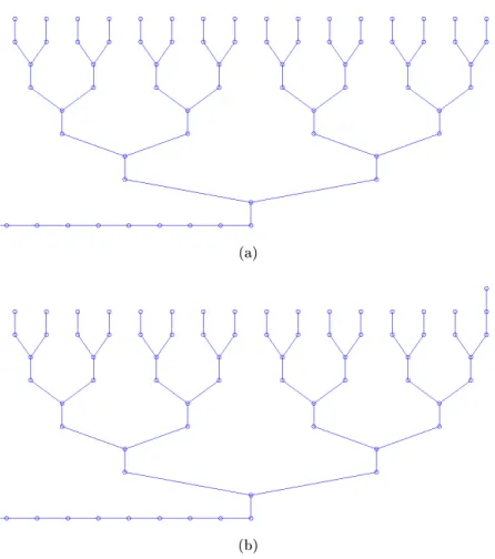
Continuous-time quantum walks are the quantum analogue of continuous-time random walks and can be used for computation. In this model, one encodes a problem in a graph, and therefore in a Hamiltonian, such that the above procedure constitutes an algorithm for the problem. To show one way in which this model can work, we briefly present (without proof) how a continuous-time quantum walk can be used to solve a Grover-type problem, formulated as computing the 𝑁-bit or function (i.e. for any 𝑁-bit input 𝑥, or(𝑥) = 0 for 𝑥 = 0 and or(𝑥) = 1 otherwise). A graph, i.e. Hamiltonian 𝐻𝑥, to solve this problem is

shown in Fig. 1-1, for the problem of distinguishing whether 𝑥 = 0 vs. 𝑥 has precisely one non-zero bit. This graph involves a “runway” attached to a modified binary tree with an extra connection on the top row of the tree depending on the input 𝑥. One can show that if the initial state is a travelling wave on the runway (specifically, ⟨𝑣|𝜓(0)⟩ ∝ 𝑒−𝑖𝑣𝜋/2 _{for 𝑣}

on the runway) and evolved for time proportional to √𝑁 under 𝐻𝑥, a measurement on the

even nodes of the last third of the runway sites yields no with high probability if 𝑥 = 0, and yes otherwise. In this way, starting with the appropriate initial state, evolving under the input-dependent Hamiltonian 𝐻𝑥, to which we assume we have access (even though we

assume we do not necessarily know the value of 𝑥), and measuring the appropriate sites, one can calculate the value of or(𝑥). Many other continuous-time quantum walk algorithms exist, and the model has been proven to be universal for quantum computation [15] (and see also a generalization in [16]).

1.2.4 Analogue Hamiltonian simulation and algorithms

While the previous models are (at least theoretically) capable of general-purpose quantum computation, we note that it may also be useful to consider quantum computing devices with more modest goals. One of the main motivations for quantum computing is quantum simulation, where we would like to study the properties of some specific quantum system, say one modelled by a Hamiltonian ˜𝐻, without having direct access to such a system. To simulate a quantum system on a classical computer is typically difficult, due to the former’s much larger state space – for example, an 𝑛-bit state has 𝑛 parameters, but to describe a generic quantum system of 𝑛 spin-1

(31)

(a)

(b)

Figure 1-1: Graphs for the 16-bit or problem for (a) an input of 𝑥 = 0000000000000000 (with an empty top row in the graph) and (b) an input of 𝑥 = 0000000000000001 (with a single node in the top row). The Hamiltonian 𝐻𝑥 consists of two parts: a runway attached

to a modified binary tree, and an input-specific part consisting of an extra vertex and edge corresponding to the location of the 1 (if any is present) in the input 𝑥. Straight edges have weight 1 and slanted edges have weight 1

4

√

2. The tree to accomplish this task was derived