Dynamic Development of Hydrofracture

HAL Id: hal-00816221

https://hal.archives-ouvertes.fr/hal-00816221

HAL is a multi-disciplinary open access archive for the deposit and dissemination of sci-entific research documents, whether they are pub-lished or not. The documents may come from teaching and research institutions in France or abroad, or from public or private research centers.

L’archive ouverte pluridisciplinaire HAL, est destinée au dépôt et à la diffusion de documents scientifiques de niveau recherche, publiés ou non, émanant des établissements d’enseignement et de recherche français ou étrangers, des laboratoires publics ou privés.

Irfan Ghani, Daniel Koehn, Renaud Toussaint, C. W. Passchier

To cite this version:

Irfan Ghani, Daniel Koehn, Renaud Toussaint, C. W. Passchier. Dynamic Development of Hydrofrac-ture. Pure and Applied Geophysics, Springer Verlag, 2013, 170 (11), pp.1685-1703. �10.1007/s00024-012-0637-7�. �hal-00816221�

Dynamic Development of Hydrofracture

Tektonophysik, Institut für Geoswissenschaften, Johannes Gutenberg Universität Mainz, Germany.

Daniel Koehn

School of Geographical and Earth Sciences, University of Glasgow, UK.

Renaud Toussaint

Institute of Globe Physics in Strasbourg, CNRS / University of Strasbourg, 5 rue Descartes, 67084 Strasbourg Cedex, France

& Centre for Advanced Study at the Norwegian Academy of Science and Letters, Drammensveien 78, 0271 Oslo, Norway.

Cees Willem Passchier

Tektonophysik, Institut für Geoswissenschaften, Johannes Gutenberg Universität Mainz, Germany.

Key Point:

Hybrid discrete-continuum formulation is developed to model natural hydro-driven fracturing. Pore pressure diffusion is crucial in pattern formation.

Abstract:

Many natural examples of complex joint and vein networks in layered sedimentary rocks are hydro-fractures that form by a combination of pore fluid overpressure and tectonic stresses. In this paper, a two-dimensional hybrid hydro-mechanical formulation is proposed to model the dynamic development of natural hydrofractures. The numerical scheme combines a Discrete Element Model (DEM) framework that represents a porous solid medium with a supplementary Darcy based pore-pressure diffusion as continuum description for the fluid. This combination yields a porosity controlled coupling between an evolving fracture network and the associated hydraulic field. The model is tested on some basic cases of hydro-driven fracturing commonly found in nature i.e., fracturing due to local fluid overpressure in rocks subjected to hydrostatic and nonhydrostatic tectonic loadings. In our models we find that seepage forces created by hydraulic pressure gradients together with poroelastic feedback upon discrete fracturing play a significant role in subsurface rock deformation. These forces manipulate the growth and geometry of hydrofractures in addition to tectonic stresses and the mechanical properties of the porous rocks. Our results show characteristic failure patterns that reflect different tectonic and lithological conditions and are qualitatively consistent with existing analogue and numerical studies as well as field observations. The applied scheme is numerically efficient, can be applied at various scales and is computational cost effective with the least involvement of sophisticated mathematical computation of hydrodynamic flow between the solid grains.

Index Terms:

0500 COMPUTATION GEOPHYSICS 0545 Modeling

0550 Model verification and validation 0560 Numerical solutions

5100 PHYSICAL PROPERTIES OF ROCKS 5104 Fracture and flow

5112 Microstructure

5114 Permeability and porosity

Keywords:

1) Introduction:

Brittle deformation of rocks in association with over pressured fluid plays an important role in the geophysical, geochemical and structural mechanics of the Earth’s crust in a wide variety of geological settings [Fyfe et al., 1978]. A number of fluid expansion mechanisms e.g., burial compaction, clay dehydration, organic matter decomposition and aquathermal expansion as well as impermeable rock units which behave as seal to subterraneous fluid flow render the

pore fluid overpressure, which if in excess of the least principal stress (P_f ₃) may lead to load

parallel or load oblique tension fracturing (figure 1) in depths of the Earth’s crust.

hydrofractures form when

T Pf 3  & 13 4T





Fig. 1: Mohr diagram of tensile failure due to fluid overpressure. The blue Mohr circle

represents the initial state of stress with zero fluid pressure. The Mohr circle moves towards the left hand side (red circles) as a result of fluid overpressure, which results in tensile/shear failure.

The mechanism of hydrofracturing has great implications in the interpretation of field observations and for the prediction of natural or industrial problems in a broad range of research

disciplines. After pioneering work of [Hubbert and Willis, 1957; Hubbert and Rubey, 1959]

which explored pore fluid pressure as an important factor for small scale hydrofracturing in tectonic processes, significant efforts have been made in the development of theoretical

fundamentals [Biot et al., 1986; J M Cleary and Illinois State Geological Survey., 1958;

Daneshy, 1973; Secor, 1965; Valkó and Economides, 1995]. Apart from theoretical aspects, a

significant amount of analytical and numerical solutions have also been put forward by many

investigators to address this coupled process in a qualitative and quantitative manner [M P

Cleary and Wong, 1985; Flekkøy et al., 2002; Gordeyev and Zazovsky, 1992; Meyer, 1986; Tzschichholz et al., 1994; Yu.N, 1993].

Most of the previous numerical tools are built on continuum approaches and consider fluid flow in fractures of simple geometry (penny-shaped elliptical or vertical cracks) using the theory of linear elasticity. Much of these approaches however, lack the constitutive relationship of explicit coupling between the solid and fluid being considered separately and makes strong approximations upon complex flow and deformation interaction arising from brittle failure, material disorder and inhomogeneity present at various scales in geo-pressurized problems.

Some porosity controlled models [Boone and Ingraffea, 1990; Flekkøy et al., 2002; Mourgues

and Cobbold, 2003; Olson et al., 2009; Wangen, 2002] revealed that the potential response of

inherent poroelastic mechanics is an important parameter in hydro-driven rock failure, where the

seepage forces caused by pore pressure gradients [Engelder and Lacazette, 1990; Rozhko, 2010;

Rozhko et al., 2007] in porous rocks affect the driving stress for fracture initiation and growth.

incorporates the dynamic coupling of at least three sub-processes [Adachi et al., 2007]; 1)

Restructuring of rock skeleton upon elastic/in-elastic strain. 2) Corresponding alteration of both the permeability and the interstitial fluid pressure. 3) Further mechanical deformation leading to fracture propagation with concurrent variation in the pore or fracture filled fluid pressure.

Inspired by [Flekkøy et al., 2002] we extended the work of [Koehn et al., 2005] to a

hybrid discrete-continuum constitutive modeling approach. The scheme emphasizes the evolution of rock failure in the light of underlying synergistic evolution of rock permeability upon fracture growth and the consequent change in interstitial pore pressure. The hypothesis is that porosity effective pore pressure diffusion along the pressure gradient is critical for the formation of discrete opening mode fractures and thus may influence the propagation of hydrofractures at large scale in porous rocks under controlled strain conditions.

The present paper evaluates the theoretical aspects of the numerical scheme for some basic configurations to which analogue and analytical studies are present i.e., hydrofracturing in homogeneous porous media under hydrostatic and non-hydrostatic conditions. In the following section we give details of the fluid-solid two-way coupling scenario of the scheme. In section 3 the validation of the solution is given and in section 4 implementations of the method is illustrated by means of simulation examples related to simple geometrical problems. Finally, results from this study are pointed out in section 5. The Alternative Direction Implicit procedure for the solution of the continuum diffusion is given in the Appendix-A.

2) Formulation

The simulations implemented in this study constitute of a special solution of the Darcy based Navier Stoke’s equation and its coupling with a discrete poroelastic medium. The basic assumption is that the poroelastic feedback is behaving according to Biot’s poroelastic theory within a linear elastic regime. This connects pore-scale force balanced hydro-physics with the evolution of the effective pressure gradient in a porous rock. Once a fracture initiates, the overall behavior of the model becomes plastic and Biot’s compressibility is no longer applicable

[Flekkøy et al., 2002]. The numerical scheme can encounter the displacement of discrete

particles or deformation of a solid matrix directly. In this way the hydrodynamics evolve intrinsically with irreversible micro deformation in a solid matrix through the use of the Kozeny-Carman porosity-permeability relation.

The solution procedure adopted for this coupled problem is based on the same basic principles that were successfully used in simulations to model instabilities in fluid filled granular

media [Johnsen et al., 2006, 2007, 2008; McNamara et al., 2000]. The same type of hybrid

models was also used to model gravitational instabilities in Rayleigh-Taylor like situations with

grains falling in a gas [J. L. Vinningland et al., 2007a, 2007b, 2009a, 2009b, 2010], or a fluid

[Niebling et al., 2010a, 2010b; Vinningland et al., 2012], and in situations of aerofracturing, i.e.

injection of gas in granular media [Niebling et al., 2012a, 2012b]. It was shown to reproduce

lubrication in sheared fault gouges due to the presence of an interstitial fluid [Goren et al., 2010,

2011] and a variant of two fluid models is used to model fluidizes beds [Jackson, 2000] and

saturated landslides [Denlinger and Iverson, 2001; Spickermann et al., 2012]. In the following

subsections we outline the idealizations employed to set up the hybrid model and describe the model components along with the formulation of constitutive equations. Then we turn to the

solution of the fluid-solid interaction, deformation mechanism and finally the assumptions made in this study.

2.1) Methodology:

The numerical scheme is built on a 2D hybrid Particle-Lattice model of unit dimension that utilizes a small-scale triangular discrete spring network code inherited from the software

‘Latte’ (part of the modeling environment ‘Elle’, [Bons et al., 2007; Koehn et al., 2005]) as a

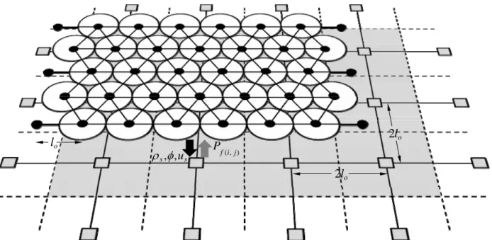
deformation isotropic porous material. The discrete lattice is then coupled with a continuum fluid phase presented by a stationary square grid of equivalent or larger dimension (figure 2).

The computation is governed by a set of two differential equations, one deals with the translation (elastic deformation) of solid particles and the second solves the time dependent diffusion of fluid pressure according to local strain rates through a poro-elasto-plastic relationship. For a given configuration of the pressure field and the solid particles, the respective constitutive equations are approximated separately by two different numerical procedures. The elastic media is relaxed by a standard over-relaxation algorithm containing kinematic boundary

conditions (n u 0) for boundary particles, while the Pressure ADI routine is used for the

solution of the pressure diffusion in a continuum grid (Appendix-A).

) , (i j f P s s,,u  o l 2 o l 2 o l

Fig 2. Schematic diagram of the hybrid hydro-elastic model, illustrates overlapping regions in

physical space comprising the DEM lattice and the continuum grid.

With a local mass to momentum conservation, the scheme embodies coupling between the solid and the Darcy continuum description. The porosity dependent evolution of the pressure gradient imparts fluid drag forces at the particles of the discrete model. Permeability is treated as an implicit fluid flow property and is an output of the discrete model as a function of change in local porosity where the change in porosity is determined by the translational movement of mass centers of the particles.

The 2D DEM model is assembled by coupling a triangular network of volume-less linear elastic springs with a particle model where disk shaped particles of constant radius superpose the nodes of the triangular structure. The particle model has its genesis from molecular dynamic models and represents the discrete quantities of the solid material, whereas following Hook’s law of interaction the spring lattice model inherits the micro-mechanical physics between the nodes. This setup thus mimics isotropic elastic behavior of solid materials and can be used to model deformation problems in systems described by linear elastic theory. The intrinsic stiffness

constant k of linear springs is related to macro-scale elastic material-parameters (E v ) through ,

the consistency measures of strain energy between the 2-D elastic lattice of the triangular

network and solid continua [Flekkøy et al., 2002].

3 2

k El (1)

where l corresponds to the thickness of the 2D particle-lattice model.

The model produces plain strain deformation and a large-scale average stress tensor can

be determined from the local deformations of elastic springs for each time stept. Springs can

break when a prescribed tensile stress threshold is overcome to exhibit discrete mode-1 fractures in the material. Broken springs are removed from the elastic network, whereas the respective particles still retain repulsive forces to accommodate the successive tension. The breaking

strength of springs is related to the mode-I stress intensity factorK , a key parameter that gives _I

stress singularities at crack tips and does depend on the size of micro cracks in the material [Flekkøy et al., 2002].

I I

K  a , (2)

where _I is the critical mode-I driving stress for the relative displacement of fracture walls and

a is the length of micro cracks in an isotropic medium. The porous model is assumed to be

homogeneous corresponding to its elastic properties on large scale, however inherent disorder ubiquitous in natural media can be quenched through characteristic distributions of material properties on particles or annealed disorder (Griffith’s micro cracks and other defects at grain scale) can be introduced by modifying the elastic properties of mechanical springs. It has been indicated that fracture patterns observed both in field and laboratory studies can be replicated by implying the realistic normal distribution of strength threshold in DEM models

[Malthe-Sørenssen et al., 1998a, 1998b; Walmann et al., 1996].

To avoid rigid body translation the elastic system is confined (closed system) by elastic walls at the boundaries. The walls behave as linear elastic springs and exercise a force on the confronted particles proportional to their distance. For instance, the force by a lateral wall on particle i contacted at xx_w is ( ) if 0 0 else w i i w i i i w i k x r x n x r x f         (3)

where r is the particle radius, _i n is a unit vector normal to the wall and _i k is a spring constant _w

for particle wall interaction.

With negligible fluid inertia, a time dependent macroscopic diffusion equation is derived that contains mass and momentum conservation in the bulk simulation of particle and continuum dynamics. The output is an interstitial fluid flow expressed in terms of a porosity dependent pressure gradient, which makes the computation simple and efficient. We start with the continuity equations (both for solid and fluid) at a characteristic scale of a grain diameter.









where _s, _f are the densities and u , _s u the velocities of the solid particles and fluid _f

respectively and  is the local porosity. The Darcy equation for the segregation of fluid and

solid gives a local fluid seepage u for a pressure drop described by the local permeability on a _f

unit area that is larger than the grain diameter.

(u_f u_s) K P





    (6)

where  and P stand for the fluid viscosity and pressure, whereas the local permeability K is

expressed as a function of the local solid fraction  according to the empirical Kozeny-Carman

relation for a Darcy like regime.

2 3 2 (1 ) ( ) 180 d K      (7)

where d is the particle diameter and 1/180 is an empirical constant valid for packing of spheres.

Similar to the quenched noise in elastic material constants, a distribution of hydraulic particle size can be treated as an epoxy to intrinsic hydraulic heterogeneity (solid fraction, permeability) in the continuum routine. In general, a larger particle area will result in low permeability and high pressure gradient and eventually an overall larger fluid drag force at the local fixed scale of

reference and vise versa. To get a fully consistent picture, the fluid adiabatic compressibility 

is included into the continuity equation according to the fluid state equation i.e., proportional approximation of the fluid density to pressure:

(1_f _o P) , (8)

where _o denotes the fluid density at some reference pressure. Substituting _f and u into _f

equation (5) and eliminate  from the subsequent equation we end up with the following _t

diffusion equation for the non-hydrostatic pressure P , with an approximation of finite solid

compressibility relative to fluid.









The left hand side of equation (9) is the Lagrangian derivative of pore pressure, the first term on the right hand side describes the Darcy diffusion of the fluid pressure relative to particles and the third term in the equation is distinguished as source term. The source term facilitates a pressure change as a function of a change in the particle solid fraction if particles move apart in the local reference scale of Darcy flow. For a detailed dimensional and non-dimensional

derivation of the continuum equation presented above see the reference [Gidaspow, 1994; Goren

The assumption of omitted fluid inertia is evident in equation (9), where the fluid flow is

described by the pressure field ( , )P x y only. This diffusive-advective description of the fluid

flow is valid when the Reynold’s number Re f

f

u d 

 is small, where  is dynamic viscosity

of the fluid, d the particle size (diameter). The Reynold’s number will be small if particles are

small as is in the considered casees of dense model. Assuming the validity of the current

approach a priori, one can also evaluate the condition of Re 1 using Darcy’s law i.e.,

2

Re ( f )

Kd _ P

   in the simulations (which is true for all the cases subjected d here). As far as

the particle movement (fracture aperture) is comparable to the diameter of particles, the above assumption of negligible fluid inertia is valid. However, if the fracture aperture becomes broader (sub-particle scale) the fluid inertia becomes important. This not only affects the particle-fluid coupling but also the fluid dynamics and in this case an equation describing the flow of fluid momentum, like the Navier-Stokes equation is required [McNamara et al., 2000]. Nevertheless, this approach is also valid for flow fields at large Reynold’s numbers [Beetstra et al., 2007].

2.4) Two way solid-continuum interaction

The DEM lattice is blanketed over the continuum grid in a way that the boundaries of the two parallelized lattices coincide with each other. With the lattice constant of the continuum grid set to be twice as large as that of the discrete lattice, this setup incorporates the “cloud in a cell” method (figure 3) to facilitate the two-way interaction between the porous matrix and the

hydrodynamic phase. The particle density  and velocity u are estimated locally on the

continuum grid in each iteration as a function of the local mean particle density specified by a linear tent weight function upon four nearest grid nodes.

 







 







where subscript i stands for particle number and the smoothing function s r





weighted distribution of particle mass relative to its position.





where r x y

 





1

w

w

i

1



i

1



j

j

j



1

1



i

Fig. 3. General overview of the twofold function of the numerical setup. Polar arrows illustrate the linear interpolation of particle area weight (grayish color code) to surrounding grid nodes and in turn the time dependent drag force from grid nodes to encountered particles.

With this configuration, the fluid drag force f on each particle encountered by a fluid _p

continuum cell can also be deduced by averaging the pressure gradient at the respective continuum node.







where k runs over four nearest grid nodes. This definition guarantees the mutual and balanced

attribution of the pressure force f to solid particles from the continuum grid and the _p

density/momentum contribution of the grains to the respective continuum unit cell as determined by equation (20) below.

In the coupled scheme, fluid pressure gradients that are approximated between fixed continuum nodes produce effective stresses at the particles of the DEM lattice. This steers the particles to displace and leads to stretching of the connected elastic springs, which ultimately break and be demonstrated as explicit fracturing when the imposed effective stress exceeds a given tensile stress threshold. Upon the formation of discrete cracks, rearrangement of the particles in the elastic medium (i.e., fracture opening) devise local changes in the background void space of the system, which in turn affects the permeability to be used in the successive step to determine the fluid pore pressure field. This evolution of fluid pore pressure again provides feedback to the stress field in the system and leads to fracture propagation or opening as a function of the particle dynamics. The procedure is repeated until both the continuity equation

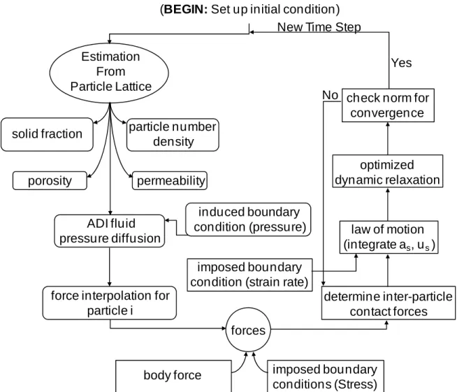
and the discrete grains are relaxed. The flowchart for one complete cycle of the algorithmic scheme is given in figure 4.

(BEGIN: Set up initial condition) New Time Step

Yes No

forces

body force imposed boundary

conditions (Stress)

check norm for convergence

force interpolation for particle i ADI fluid pressure diffusion porosity permeability particle number density solid fraction Estimation From Particle Lattice induced boundary condition (pressure) determine inter-particle contact forces imposed boundary

condition (strain rate)

law of motion

(integrate as, us )

optimized dynamic relaxation

Fig. 4. Flowchart for the complete cycle of the algorithmic scheme.

2.5) Deformation mechanics

The translation motion of the initially relaxed solid particles (solid-solid interaction) is

managed by the momentum exchange between solid and fluid phases in a unit volume cell dV

(with unit third dimension) of the coupled system on account of-the inter-particle contact force

e

f (either connected with a spring or repulsive force), fluid force f and gravity loadingp f . g

e p g

dV

m f f f

dt           (14) 

where the forces fe being aligned along the connected elastic springs are characterized by spring

constant kij times the actual distance between the centroid of the particles minus the equilibrium

distance a_ij.





e ij ij i j ij j

where x_i and x_j are the positions of the connected particles, ˆn_ij is unit vector pointing from the

centroid of particle i to particle j and the sum runs over all the connected neighbors j . The

fluid force f that acts on the surface normal _p dA of the unit cell is a result of the fluid flow due

to the pressure gradient and is given as:

p

f  



where P is the local fluid pressure, which is the sum of the hydrostatic pressure _fgz and

extraneous pressureP . The term gravitational force _o f incorporates the gravity effects of both _g

the fluid and solid masses where the former together with the hydrostatic part of pressure determines the effective stress _eff (_s _f)gz on the solid particles.

g s f

f   dV g   dV g (17)

In the geological realm a transient hydrofracturing is likely to take place by a pore

pressure P in excess to _eff . However, for the considered linear elastic model that exhibits

deformation in a quasi-static fashion we only need to assume pore pressure deviations from the lithostatic pressure. This has been achieved by introducing the effect of gravity in form of lithostatic stress and results in the calculated stresses minus the lithostatic pressure. The inferred

gravity force on a single cylindrical particle i of volume V_s r h2 with base area A_s r2,

where h1 is the thickness in the third dimension is:

2 g i s i f  R gs (18) with 2 3 m m R R E A s E A  (19)

where _s is the material mass density, R_i   with r_i S S the dimension of the real system. E , _m

R

E and A , _m A stand for the Young’s Moduli and areas of particles in the model and the real _R

system respectively. The factor 2/3 in equation (19) is derived using the expedient strain-stress relation ( _{v (1 )(1 2 )}E ₍₁E(1_{)(1 2 )}) _v h              

  ) from the generalization of Hooke’s law for a 2D plane

strain problem assuming  1 / 3 and zero lateral deformation. This is essential in order to

acquire a compatible one dimensional lithostatic stress _v gh for the isotropic 2D linear

elastic solid.

By considering the local fluid velocity a rival of the local particle velocity i.e., high viscous fluid and substituting the respective constitutive force terms in equation (14) one can derive the following force-balance equation, which exhibits an explicit coupling between

granular motion and fluid flow in the unit cell ( 1

n dV  _ ).





where _n is the particle number density, _eff _s_f is the effective mass density and g the

the absence of any frictional and tangential effects. The mass m in the left term accounts for the _s

summation of fluid mass to each individual solid particle as a function of the local porosity to particle number density ratio.

2.6) Assumptions

The assumptions made in order to keep the proposed scheme amenable are:

 The fluid-solid friction force at the surface of the solid particles is not considered,

therefore the pressure gradient P is the only agent that produces a drag force (in the

direction of fluid flow) on particles.

 The fluid is considered to be purely viscous and therefore any effect like thermal evolution of the fluid (a pivotal factor in the development of subsurface overpressure e.g., dehydration of sediments in intrusive zones in particular) is not taken into account.

 The locally interpolated solid fraction on the 2D continuum grid is multiplied by 2/3. With this factor we obtain a good mapping of the 2D porosity on the corresponding 3D equivalent (prerequisite for the 3D Kozeny-Carman permeability) with a match between closed packed configurations and the empty configurations [McNamara et al., 2000]. Without this correction the qualitative behavior is comparable but quantities like fracture speed, propagation or the flux for certain pressure gradients can change by a prefactor, roughly up to a factor 2.

 Analytically the Kozeny-Carman relation works as long as the solid fraction is greater than zero, but a solid fraction of 0.15 or less presents a solid-fluid composite mainly as a fluid and is thus inconsistent with the Kozeny-Carman relation (originally established for dense granular media). We thus chose to apply a threshold to a permeability of a medium with a solid fraction of 0.15 (e.g., in a broader fracture aperture). The main purpose of limiting the solid fraction and hence permeability to this upper value is to allow larger time steps and improve the speed of the model. Effectively, the zones of the model where the permeability is equal to large values correspond to almost homogeneous pressure zones. The exact value of this cutoff does not affect the pattern formation significantly, as different values of the cutoff have been tested (between 0.25 and 0.05) without any significant changes [Johnsen et al., 2006; Jan Ludvig Vinningland et al., 2007a].

3) Model verification

We first test the linearity of the porosity controlled Darcy flow field and the associated pressure forces on each particle. If we consider compressible water as fluid in the pore space, the evolution of seepage forces in the simulations (figure 5) validates the theoretical aspects of the scheme. A reference model of unit dimension is taken as a porous rock where the solid skeleton is composed of 11500 disc-shaped adhesive particles. The system is confined mechanically at all boundaries whereas hydraulically it is restrained only at the side boundaries. Neglecting any gravitational loading a hydraulic gradient i is established in the system by setting the bottom

boundary at a constant pressure input (normalized P1.0) and fixing the top boundary at 0.0

pressure respectively. The pressure input value is kept suitably low in order not to produce fractures.

Two series of simulations are conducted to test the model by considering a homogeneous (figure 5a) and a heterogeneous (figure 5b) porous rock respectively. In the heterogeneous case a seal is inserted in the model. The seal is represented by a horizontal layer of low permeability

with a thickness of 0.1 with lower boundary at 0.2 and upper boundary at 0.3. In the test simulations, initially a high pressure gradient is concentrated in the vicinity of the source boundary, therefore only the intimate particles are subject to resultant seepage forces and consolidate along the direction of the pressure drop. However, after 5000 time steps the pressure gradient becomes linear and the fluid approaches a steady state flow condition in the homogeneous model. In the heterogeneous medium a strong pressure drop develops across the layer of relative low permeability. Two linear regimes develop, one below the seal with a relatively steep gradient and one above the seal with a relatively gentle gradient. Consequently vertical seepage forces of high contrast in magnitude are measured at the seal boundaries (figure 6). 0 0.2 0.4 0.6 0.8 1 0 0.2 0.4 0.6 0.8 1 0 0.2 0.4 0.6 0.8 1 P X Y P a) Time: 100 0 0.2 0.4 0.6 0.8 1 0 0.2 0.4 0.6 0.8 1 0 0.2 0.4 0.6 0.8 1 P X Y P b) Time: 100 0 0.2 0.4 0.6 0.8 1 0 0.2 0.4 0.6 0.8 1 0 0.2 0.4 0.6 0.8 1 P X Y P a) Time: 1000 0 0.2 0.4 0.6 0.8 1 0 0.2 0.4 0.6 0.8 1 0 0.2 0.4 0.6 0.8 1 P X Y P b) Time: 1000 0 0.2 0.4 0.6 0.8 1 0 0.2 0.4 0.6 0.8 1 0.2 0.4 0.6 0.8 1 P X Y P a) Time: 5000 0 0.2 0.4 0.6 0.8 1 0 0.2 0.4 0.6 0.8 1 0 0.2 0.4 0.6 0.8 1 P X Y P b) Time: 5000

Fig. 5. Normalized pore pressure profiles at different time steps, (a) in a homogeneous porous medium, (b) in a heterogeneous porous medium accompanying a horizontal seal of low porosity

at position 0.2 0.3 on the y-axis (vertical axis).

T 0 0.2 0.4 0.6 0.8 1 Fy seal (y = 0.2) seal (y = 0.3) no seal (y = 0.2) no seal (y = 0.3)

Fig. 6. Overall evolution of the vertical seepage forces as a function of time (T:1000) for a homogeneous system and at the lower and upper boundary contacts of the seal in a heterogeneous system. The forces display a sharp contrast in magnitude in the heterogeneous case, whereas in the homogeneous medium the forces show a gradual increase in pressure force. Both the heterogeneous and homogeneous cases reach a steady state condition.

4) Model implementation

In the following sections we show two different test cases to illustrate the development of hydro-fractures in the model.

 Foremost, we discuss fracturing in a homogeneous medium where fractures develop around a point source (fluid is injected locally) in the absence of external deformation. We investigate the fracture pattern that develops as a function of fluid pressure gradients under isotropic diffusion of the fluid pressure. In addition we analyze the influence of changes in background porosity and study the state of stress during fracturing in detail. Later, the likely influence of background non-hydrostatic stress states (i.e., uniaxial vertical loading and pure shear deformation) on the growth of hydrofracture is also examined.

 In the second set of two simulations, we advance to simulate fracture patterns due to local pressure sources in the presence of gravity and tectonic strains. In these cases we use examples where seepage forces develop due to a local increase in pore pressure caused by local perturbations in the stress state. In this case the tectonic strain conditions will control the different fracture patterns.

In each test the model starts from a fully relaxed state and is loaded in small steps afterwards. According to the boundary conditions loading includes increase of fluid pressure in

the fluid lattice, vertical loading due to gravity or horizontal loading due to tectonic strains by moving the boundary walls. The mechanical and hydraulic boundary conditions vary accordingly with respect to the underlying problem to imitate laboratory and field conditions.

4.1) Point source in a homogeneous porous medium

In these simulations the fluid pressure is increased at a point source with a constant rate (P

t

 ) at the centre of a homogeneous and isotropic poro-elastic domain. The model is

mechanically confined and bears no-flow boundary conditions. In these simulations the hydrofracturing process shows two stages, fracture initiation and episodic fracture growth until the system reaches a steady state (Fig. 7).

The accumulation of fluid pressure at the point source generates an isotropic pressure gradient in the surrounding which contributes to the evolution of the effective stresses and deforms the porous rock elastically as a function of Biot’s poro-elastic coefficient. The rock experiences micro fracturing from the concentration of stress on relatively weak rock elements. The discrete fractures nucleate at the source location and tend to propagate into the undisturbed region (Fig. 7a). At this stage, tension cracking accommodates the strain in the system and results in stress relief and a potential local change in porosity when particles are pushed away by the pressure force and fractures open. This cycle is repeated following the two-way temporal and spatial feedback between hydraulic pressure field and elastic field on account of induced fracturing in the porous matrix until a steady state condition is acquired and fracturing ceases. The symmetry of the developing fracture pattern at the point of injection is a function of a circular extension around the fluid source. The symmetric pattern validates the homogeneous existence of pore pressure in the rock matrix. The seepage forces that develop due to the pressure diffusion modify the force balance in the porous rock sample, which deterministically drives the discrete tensile crack growth along the pressure gradient and results in a regular fracture geometry.         T: 100 T: 100

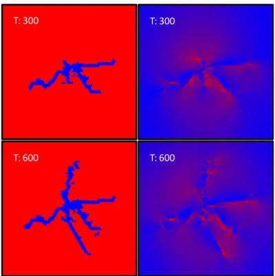
T: 300 T: 300

T: 600 T: 600

Fig. 7a. The figures on the left hand side show the development of circular hydro-fractures (T= model time, blue particles have broken bonds) by a point source overpressure. The figures on the right hand side show the same simulations and illustrate the associated differential stress states of the model at the respective failure stages (red=high; blue=low differential stress).

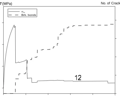
Figure 7b shows the evolution of the effective mean stress in the model (positive mean stress is extensional) as a function of time and the growth of broken bonds with time for the simulation shown in figure 7a. In the first steps of the model the effective mean stress increases in a non-linear fashion due to the diffusive nature of the pore fluid pressure. Once the tensile strength of the material is reached the rock fractures suddenly and the stress drops significantly. Subsequently the stress increases slowly, which is followed by subsequent failure events. Finally fracture growth ceases and the mean stress reaches a steady state. Because the shown stress is an average of a larger area in the model the fracturing continues locally even though the mean stress has already reached equilibrium.

(MPa)

 No.ofCracks

t

Fig. 7b. Graph shows oscillations in effective mean stress and associated number of broken bonds in the model. The stress shows the episodic evolution of the fluid pressure. Positive effective mean stress in the model is defined as extensional stress.

(MPa)

m 

t

Fig. 8. Mean stress as a function of background rock porosity, where an increase in porosity results in a lower driving force because the pressure can diffuse faster. Note: –ve sign in the model is annotated for compressive stress and +ve sign for extensional stress.

Under the same fluid injection rate a quantitative comparison of the mean stresses in rock samples with different background porosities is given in figure 8. The graphs in figure 8 show the evolution of the effective mean stress field and the fracturing behavior of the rock as a function of porosity. Rocks that inherit low porosity entail the production of high seepage forces to drive tensile failure at comparable low average tensile stress. A low average stress illustrates that the stress in a low porosity rock will be very localized around the point source. The stress drop associated with failure of the material will be relatively large. In addition the state of stress

may be altered in these low porosity rocks due to friction along developing fractures (solid-solid coupling), where the overall stress regime may become compressive (figure 8). Subsequently small isolated shear or hybrid extension-shear fractures can develop near the end of the primary dilational fractures when fracturing happens relatively early in low porosity rocks. When the porosity becomes larger the initial loading of the system due to the fluid input becomes successively more non-linear (Fig. 8) up to a point where the pressure just diffuses out of the system without the creation of fractures.

We also simulated a number of examples (Appendix-B, Appendix-C) with the similar hydraulic setup but different external boundary conditions. The developing fracture patterns closely resemble the results observed experimentally by [Bruno and Nakagawa, 1991; Doe and

Boyce, 1989] in rock type material. The simulations manifest the effective influence of pore

pressure on the likelihood of tensile failure and the corresponding fracture propagation under non-hydrostatic stress conditions in homogenous sedimentary rocks.

4.2) Hydrofracturing in a homogeneous medium under gravity loading

In the second set of simulations, we reproduce the patterns of hydrofracturing caused by a local pore fluid overpressure under non-hydrostatic tectonic loadings of gravity and lateral stresses and found the results consistent with [Rozhko et al., 2007]. The problem is analogous to various geological systems (magmatic intrusions, hydrothermal venting, volcanoes etc.), which yield a local perturbation in the effective stress field with the induction of localized pore overpressure.

Figures 9 and 10 show simulations with a local point source at the bottom of the model, where the former sustains a stress regime of horizontal extension and the later horizontal compression. The model material is homogeneous and the gravitational loading is followed by equation (18). In order to incorporate the effect of gravitational loading, the model is subjected to a two-stage deformation in both cases. First, the model is let to settle under uniaxial gravitational

loading assuming the model is 1 km in depth with fixed side walls, a rock density of 2.5 kg/m3,

Young modulus of 80GPa and Poisson ratio of 1/3. This setup yields a global stress anisotropy where vertical and horizontal stresses differ due to Poisson effects. Secondly, we apply a lateral extension or compression with a relative small horizontal strain rate in order to have a fluid dominated effective state of stress in the rock. A hydraulic anisotropy is produced in the simulations by inducing a pressure drop with a zero assigned pressure at the upper boundary and no flow boundary conditions at the side-walls.

Str ai n  co nt ro ll ed /  im pe rm ea bl e  bounda ry Stress controlled boundary Free boundary Str ai n  co ntr ol le d/  im pe rm ea b le   bou nda ry

Fig. 9. Vertical hydrofracture in a rock model subjected to lateral extensional strain. A vertical gravitational load is applied to the system and fluid is injected at a point source in the middle of the system at the lower boundary.

Str ai n co nt ro lle d/  im pe rm e abl e  bound ar y Str ai n co n tr ol le d/  im p erm e ab le   bounda ry Stress controlled boundary Free boundary

Fig. 10. Conjugate shear fractures under compressive state of stress. A vertical gravitational load is applied to the system and fluid is injected at a point source in the middle of the system at the lower boundary.

The system that is loaded with a gravitational body force experiences buoyancy forces

i.e., P(_s_f)gz in equation (9) with the reduction in effective stresses due to an increase in

local pore pressure. This gradient may lead to a quasi-static fracture propagation through parts of the model.

The failure patterns illustrated in figures 9 and 10 are consistent with the different forces that are applied. Fracturing nucleates in the areas where fluid pressures are high (point source at the bottom of the models). The fractures propagate upwards reflecting the gravitational loading of the system. The horizontal tectonic forces produce almost vertical extensional mode I crack like failure when the system is extending (figure 9) and conjugate shear failure when the system is under compression (figure 10). Even though the source of the fracturing is a high fluid pressure in both cases the pattern that develops is strongly influenced by the heterogeneous stress field due to gravity and tectonic loading. This is clearly illustrated when figure 7a is compared, since figure 7a has the same fluid boundary condition with a point source as figures 9 and 10 but the fracture pattern is very different in the later cases due to the external stress field.

Discussion and conclusion

Discrete fractures or instant opening of existing cracks as a function of fluid overpressure drive perturbations in permeability, change the state of stress and the corresponding release of strain energy on the scale of pores. In this contribution we present a hybrid numerical solution based on first principles rather than on empirical constitutive relationship with ad hoc fitting parameters to model natural examples of hydrofractures. First principles constitute the equation of state separately for the fluid and the solid and the pore scaled forces balance to describe interactions. The scheme thus combines the pertinent features of both continuum and DEM descriptions, and examines the dynamic coupling between porous flow and diagenetic process through fracture mechanics as a response to an applied pressure gradient across the system.

It appears likely that the interplay between the temporal and spatial evolution of the pore pressure and tectonic/gravitational stresses manipulate hydro-fracturing and the corresponding permeability changes. Our model shows an evolution of the deformation dependent permeability illustrating that in hydro-mechanical systems permeability is a nonlinear and time dependent parameter where fracturing localization is very important. The system reacts to forcing and produces the permeability that it needs to allow the fluid pressure to diffuse. It has manifested that small-scale diagenetic events can have adequate impact on the pressure field and in turn the fracture geometry. In our model this effect is achieved by the idealized hydro-mechanical constitutive relation of Kozeny-Carman permeability through a weighted interpolated function. In this relation even small displacements of particles can lead to significant changes in the local solid density and thus the Darcy fluid flow.

It has been perceived that several key features (flow rate upon compaction, yield surface, strain softening and hardening etc.) of critical soil mechanics (CSSM) are inconsistent with the observed porosity and pressure dependent deformation behavior of porous rocks [Cuss et al., 2003; Gerogiannopoulos and Brown, 1978; Ling et al., 2002; Wong et al., 1992; Wong et al., 1997]. Therefore, the use of Kozeny-Carman relation (originally developed for soils) for the evolution of the permeability field in the presented model is justified. However, concerns may rise where porosity-permeability relations deviate from the trend of the basic equation [Zhu and

Wong, 1997] e.g., fracturing in subsurface impermeable rocks causes enhancement in the

permeability in contrast to permeable rocks which bear a reduction in permeability. In this case one can pursue either of the following two ways:

1. Use different modified forms of the permeability dependence on the porosity both for ductile and brittle dominated deformation zones using the assumption of linearity

between porosity and log permeability with defined parametric values from experimental data [Sheldon et al., 2006].

2. When approximating the local dimension of induced fracture (aperture), a modified form of the porosity-permeability relationship can be derived from the cubic law of fluid flow in fractures [Steefel and Lasaga, 1994].

The simulated results validate the generality of the scheme implying that linear Darcy flow has an effective factor in the process of hydrofracturing, and the results are in good agreement with previously reported laboratory and field studies. The numerical scheme can qualitatively replicate some typical quasi-static field examples of hydrofractures when different modeling approaches are applied. Representative example problems constitute fracturing in homogeneous and heterogeneous porous rocks analogous to hydraulic fracturing in pressurize boreholes and natural fracture patterns due to local fluid overpressure. Simulation results illustrate that the diffusion of fluid pressure is a crucial mechanism that interacts with the effective stress field under different geological conditions and produces fracture geometries like branching fractures at point sources, vertical and shear hydrofractures under tensional/compressional tectonic settings.

The presented routine defines a fast approach both for qualitative and quantitative estimation of hydro-driven deformation problems at micro scale. The method can also be used to analysis large scale problems with the suitable selection of none dimensional parameters. In general, gravity loading and the associated non-hydrostatic stress fields along with mechanical heterogeneity in the lithology can have a vital influence over the evolution of buoyant effective forces and thus the hydrofracture patterns. Therefore future work will attempt to integrate these physical parameters in order to determine the appropriate geological conditions when analyzing natural vein and joint networks in real reservoirs.

The presented scheme is also capable to model 3D hydrofracturing, which may have more significant advantages in understanding the complex growth of fractures under the influence of 3D heterogeneity and non-hydrostatic conditions. The only change required is the interpolation of local mass density and velocity over a cubical unit volume of a 3D continuum grid using the same assigned tent function. In the future we intend to couple the derived continuum code with a newly developed 3D next-nearest particle lattice code “Melange” [Sachau and Koehn, in press].

Appendix-A: ADI - 2D Pressure Diffusion

The ADI method is time implicit. With symmetric discretization in time i.e., between a forward and backward step, this methods is unconditionally stable and the precision is better than with a purely forward in time implicit method [Press, 1992].

The two-dimensional pressure diffusion equation (9) can be rewritten as P(r,t) t  1





where g(r,t) is the source term and r stands for position in space. This is a second-order parabolic partial differential equation.

Corresponding to the time and space discretization of the 2D pressure continuum using forward difference with time on the left-hand side and central difference with space on the right hand side of equation (A1). 1 2 , , , 1, , 1, , 1 , , 1 , 2 2 , 2 2 ₁ (1 ) ( ) ( ) n n i j i j i j i j i j i j i j i j i j i j i j P P k P P P P P P P g t   x y                _  _  _   _ (A2)

where ,i j and n are the indices in the x, y, and t directions respectively.

The main idea of the ADI method is to reduce the 2-D problem into a succession of two

one-dimensional problems by proceeding one time step from n to n1 in two sub-time steps (figure

i). The first half-step (n to 1

2

n ) is taken implicitly in the x-direction and explicitly in the

y-direction followed by the second half-step ( 1

2

n to n1) that is taken implicitly in the

y-direction and explicitly in the x-y-direction.

i = 0…..I _{Step I: x-direction implicit}

Step II: y-direction implicit

1 2 1, n i j P_ 12 , n i j P  12 1, n i j P_ 1 , 1 n i j P _ 1 , n i j P  1 , 1 n i j P _

Fig. (I). Schematic diagram of ADI solution of Finite-difference pressure continuum, after [Wang and Chen, 2001].

Detailed differential equations in stage-1 for each j at marched time 1 2

n and the

corresponding tridiagonal system of equations for the respective one-dimensional problem can be derived in form of matrix equation of dimension I:

1 1 1 2 2 2 , 1, (1 2 , ) , , 1, , , 1 (1 2 , ) , , , 1 , 2 n n n n n n i j i j i j i j i j i j i j i j i j i j i j i j i j t P P P P P P g                         (A3) 1 2 1 2 1 2 0, , , , 1, , , , , , , , 1 0 0 ... ... 0 1 2 0 ... ... 0 ... ... ... ... 0 ... ... ... 0 1 2 ... 0 ... ... 0 0 1 1 0 0 ... ... 0 1 2 0 ... ... 0 ... ... ... ... 0 ... ... 0 n j n i j i j i j j i j i j i j n I j i j i j i j P P P                   _{  } _{ }  _{ }  _{ }  _{  }     _{ }    _{  }  ,0 ,1 , , 1, , , ... 2 1 2 ... 0 ... ... 0 0 1 n i n i i j i j j i j n i J P P t g P                 _         _              (A4) 0,1,..., ; 0,1,..., i I j J where , , , 2 , 2 , , (1 ) and (1 ) 2 ( ) 2 ( ) i j i j i j i j i j i j K t K t P P x y              

By analogy, stage-II of the ADI method for each i at time n1, is expressed in tridiagonal

system of dimension J: 1 1 1 2 2 2 , , 1 (1 2 , ) , , , 1 , 1, (1 2 , ) , , 1, , 2 n n n n n n i j i j i j i j i j i j i j i j i j i j i j i j i j t P P P P P P g                         (A5) 1 ,0 1 , , , ,1 , , , 1 , , , , , 1 0 0 ... ... 0 1 2 0 ... ... 0 ... ... ... ... 0 ... ... ... 0 1 2 ... 0 ... ... 0 0 1 1 0 0 ... ... 0 1 2 0 ... ... 0 ... ... ... ... 0 ... ... 0 1 n i n i j i j i j i i j i j i j n i J i j i j i j i j P P P                    _{  }              _{  }               1 2 1 2 1 2 0, 1, , , , , ... 2 2 ... 0 ... ... 0 0 1 n j n j i j i j i j n I j P P t g P          _{ }  _{ }  _{  }  _{ }  _     _{ }    _{  } (A6) 0,1,..., ; 0,1,..., i I j J

Implementing the Gauss-algorithm with a Dirichlet boundary condition, the derived tridiagonal

Appendix-B: Fr ee  b oun da ry (a) Strain controlled boundary (     )y Strain controlled boundary (     )y Fr ee  b oun da ry Fr ee  bo un da ry (b) Strain controlled boundary (     )y Strain controlled boundary (     )y Fr ee  bo und ar y (c) Strain controlled boundary (     )y Strain controlled boundary (     )y   Fig. (II). Different patterns of hydro-fractures in a situation where a constant point source is

injected in a homogeneous media under different remote stresses: (a) with relative smaller  , _y

the results show the initial development of circular fracturing at the source location (centre) with elongated fractures oriented parallel to the axis of the applied stress. In contrast to the pattern

shown in (a), in (b) a larger  dominates the overall pattern and results only in sub-vertical _y

oriented fractures parallel to the main stress axis and through the source location (central). (c) The figure shows the state of stress field at the onset of fracturing, where the red color code represents high differential stress and blue low differential stress.

Appendix-C: Str e ss  c o nt ro lle d  bo un d ar y Strain controlled boundary (     )y Strain controlled boundary (     )y T: 1100 Str e ss  c o nt ro lle d  bo un d ar y Str es s co n tro lle d bo un da ry Strain controlled boundary (     )y Strain controlled boundary (     )y T: 1200 Str e ss  c o nt ro lle d  bo un d ar y Strain controlled boundary (     )y Strain controlled boundary (     )y T: 1250   Fig. (III). This figure shows a time series illustrating the influence of the local pore overpressure on brittle failure in a pure shear stress regime. In this case the extension fractures develop at the source location (centre) and link up with shear fractures onwards the edges of the simulation box (time steps T increase from left to right).

We are deeply grateful to Till Sachau for his valuable discussions. This study was carried out within the framework of DGMK (German Society for Petroleum and Coal Science and Technology) research project 718 "Mineral Vein Dynamics Modelling", which is funded by the companies ExxonMobil Production Deutschland GmbH, GDF SUEZ E&P Deutschland GmbH, RWE Dea AG and Wintershall Holding GmbH, within the basic research program of the WEG Wirtschaftsverband Erdöl- und Erdgasgewinnung e.V. We thank the companies for their financial support and their permission to publish these results.

References

Adachi,  J.,  E.  Siebrits,  A.  Peirce,  and  J.  Desroches  (2007),  Computer  simulation  of  hydraulic  fractures,  International Journal of Rock Mechanics and Mining Sciences, 44(5), 739‐757. 

Beetstra,  R.,  M.  A.  van  der  Hoef,  and  J.  A.  M.  Kuipers  (2007),  Drag  force  of  intermediate  Reynolds  number flow past mono‐ and bidisperse arrays of spheres, AIChE Journal, 53(2), 489‐501. 

Biot, M. A., L. Masse, and W. L. Medlin (1986), A Two‐Dimensional Theory of Fracture Propagation, SPE  Production Engineering, 1(1), 17‐30. 

Bons, P. D., D. Koehn, and M. W. Jessell (2007), Microdynamics Simulation, Springer. 

Boone,  T.  J.,  and  A.  R.  Ingraffea  (1990),  A  numerical  procedure  for  simulation  of  hydraulically‐driven  fracture propagation in poroelastic media, International Journal for Numerical and Analytical Methods in  Geomechanics, 14(1), 27‐47. 

Bruno,  M.  S.,  and  F.  M.  Nakagawa  (1991),  Pore  pressure  influence  on  tensile  fracture  propagation  in  sedimentary  rock,  International  Journal  of  Rock  Mechanics  and  Mining  Sciences  &  Geomechanics  Abstracts, 28(4), 261‐273.  Cleary, J. M., and Illinois State Geological Survey. (1958), Hydraulic fracture theory, [s.n.], Urbana.  Cleary, M. P., and S. K. Wong (1985), Numerical simulation of unsteady fluid flow and propagation of a  circular hydraulic fracture, International Journal for Numerical and Analytical Methods in Geomechanics,  9(1), 1‐14.  Cuss, R. J., E. H. Rutter, and R. F. Holloway (2003), The application of critical state soil mechanics to the  mechanical  behaviour  of  porous  sandstones,  International  Journal  of  Rock  Mechanics  and  Mining  Sciences, 40(6), 847‐862. 

Daneshy,  A.  A.  (1973),  On  the  Design  of  Vertical  Hydraulic  Fractures,  SPE  Journal  of  Petroleum  Technology, 25(1), 83‐97. 

Denlinger,  R.  P.,  and  R.  M.  Iverson  (2001),  Flow  of  variably  fluidized  granular  masses  across  three‐ dimensional terrain 2. Numerical predictions and experimental tests, J. Geophys. Res., 106(B1), 553‐566.  Doe,  T.  W.,  and  G.  Boyce  (1989),  Orientation  of  hydraulic  fractures  in  salt  under  hydrostatic  and  non‐ hydrostatic stresses, International Journal of Rock Mechanics and Mining Sciences & Geomechanics  Abstracts, 26(6), 605‐611. 

Engelder,  T.,  and  A.  Lacazette  (1990),  Natural  hydraulic  fracturing,  paper  presented  at  Rock  Joints:  Proceedings of the international symposium on rock joints, A.A. Balkema, Rotterdam, Loen, Norway.  Flekkøy, E. G., A. Malthe‐Sorenssen, and B. Jamtveit (2002), Modeling hydrofracture, J Geophys Res‐Sol  Ea, 107(B8). 

Fyfe,  W.  S.,  N.  J.  Price,  and  A.  B.  Thompson  (1978),  Fluids  in  the  earth's  crust:  their  significance  in  metamorphic, tectonic, and chemical transport processes, Elsevier Scientific Pub. Co. 

Gerogiannopoulos, N. G., and E. T. Brown (1978), The critical state concept applied to rock, International  Journal of Rock Mechanics and Mining Sciences & Geomechanics Abstracts, 15(1), 1‐10. 

Gidaspow,  D.  (1994),  Multiphase  Flow  and  Fluidization:  Continuum  and  Kinetic  Theory  Descriptions,  Academic Press. 

Gordeyev, Y. N., and A. F. Zazovsky (1992), Self‐similar solution for deep‐penetrating hydraulic fracture  propagation, Transport in Porous Media, 7(3), 283‐304. 

Goren,  L.,  E.  Aharonov,  D.  Sparks,  and  R.  Toussaint  (2010),  Pore  pressure  evolution  in  deforming  granular material: A general formulation and the infinitely stiff approximation, J. Geophys. Res., 115(B9),  B09216. 

Goren,  L.,  E.  Aharonov,  D.  Sparks,  and  R.  Toussaint  (2011),  The  Mechanical  Coupling  of  Fluid‐Filled  Granular Material Under Shear, Pure and Applied Geophysics, 168(12), 2289‐2323. 

Hubbert,  M.  K.,  and  D.  G.  Willis  (1957),  Mechanics  Of  Hydraulic  Fracturing  Petroleum  Transactions,  AIME, 210, 153‐168.  Hubbert, M. K., and W. W. Rubey (1959), Role Of Fluid Pressure In Mechanics Of Overthrust Faulting: I.  Mechanics of Fluid‐Filled Porous Solids And Its Application To Overthrust Faulting, Geological Society of  America Bulletin, 70(2), 115‐166.  Jackson, R. (2000), The Dynamics of Fluidized Particles, Cambridge University Press.  Johnsen, R. Toussaint, K. J. Måløy, and E. G. Flekkøy (2006), Pattern formation during air injection into  granular materials confined in a circular Hele‐Shaw cell, Physical Review E, 74(1), 011301.  Johnsen, R. Toussaint, K. J. Måløy, E. G. Flekkøy, and J. Schmittbuhl (2007), Coupled air/granular flow in  a linear Hele‐Shaw cell, Physical Review E, 77(1), 011301.  Johnsen, C. Chevalier, A. Lindner, R. Toussaint, E. Clement, K. J. Maloy, E. G. Flekkoy, and J. Schmittbuhl  (2008),  Decompaction  and  fluidization  of  a  saturated  and  confined  granular  medium  by  injection  of  a  viscous liquid or gas, Phys Rev E Stat Nonlin Soft Matter Phys, 78(5 Pt 1), 6. 

Koehn, D., J. Arnold, and C. W. Passchier (2005), Fracture and vein patterns as indicators of deformation  history: a numerical study, Geological Society, London, Special Publications, 243(1), 11‐24. 

Ling, H., D. Yue, V. Kaliakin, and N. Themelis (2002), Anisotropic Elastoplastic Bounding Surface Model  for Cohesive Soils, Journal of Engineering Mechanics, 128(7), 748‐758. 

Malthe‐Sørenssen,  A.,  T.  Walmann,  B.  Jamtveit,  J.  Feder,  and  T.  Jøssang  (1998a),  Modeling  and  characterization of fracture patterns in the Vatnajökull glacier, Geology, 26(10), 931‐934. 

Malthe‐Sørenssen, A., T. Walmann, J. Feder, T. Jøssang, P. Meakin, and H. H. Hardy (1998b), Simulation  of extensional clay fractures, Physical Review E, 58(5), 5548‐5564. 

McNamara,  S.,  E.  G.  Flekkøy,  and  K.  J.  Måløy  (2000),  Grains  and  gas  flow:  Molecular  dynamics  with  hydrodynamic interactions, Physical Review E, 61(4), 4054‐4059. 

Meyer, B. R. (1986), Design Formulae for 2‐D and 3‐D Vertical Hydraulic Fractures: Model Comparison  and Parametric Studies, in SPE Unconventional Gas Technology Symposium, edited, 1986 Copyright 1986  Society of Petroleum Engineers, Inc., Louisville, Kentucky. 

Mourgues,  R.,  and  P.  R.  Cobbold  (2003),  Some  tectonic  consequences  of  fluid  overpressures  and  seepage forces as demonstrated by sandbox modelling, Tectonophysics, 376(1–2), 75‐97. 

Niebling,  M.  J.,  E.  G.  Flekkoy,  K.  J.  Maloy,  and  R.  Toussaint  (2010a),  Mixing  of  a  granular  layer  falling  through a fluid, Phys Rev E Stat Nonlin Soft Matter Phys, 82(1 Pt 1), 7. 

Niebling, M. J., E. G. Flekkøy, K. J. Måløy, and R. Toussaint (2010b), Sedimentation instabilities: Impact of  the fluid compressibility and viscosity, Physical Review E, 82(5), 051302. 

Niebling,  M.  J.,  R.  Toussaint,  E.  G.  Flekkøy,  and  K.  J.  Måløy  (2012a),  Dynamic  aerofracture  of  dense  granular packings, Physical Review E 86, 061315. 

Niebling, M. J., R. Toussaint, E. G. Flekkøy, and K. J. Måløy (2012b), Numerical studies of aerofractures in  porous media, Revista Cubana de Fysica 29, 1E, 1E66. 

Olson,  J.  E.,  S.  E.  Laubach,  and  R.  H.  Lander  (2009),  Natural  fracture  characterization  in  tight  gas  sandstones: Integrating mechanics and diagenesis, AAPG Bulletin, 93(11), 1535‐1549. 

Press, W. H. (1992), Numerical recipes in C: the art of scientific computing, Cambridge University Press.  Rozhko, A. Y. (2010), Role of seepage forces on seismicity triggering, J Geophys Res‐Sol Ea, 115.