HAL Id: hal-02403259
https://hal.archives-ouvertes.fr/hal-02403259
Submitted on 31 May 2021
HAL is a multi-disciplinary open access archive for the deposit and dissemination of sci-entific research documents, whether they are pub-lished or not. The documents may come from teaching and research institutions in France or abroad, or from public or private research centers.
L’archive ouverte pluridisciplinaire HAL, est destinée au dépôt et à la diffusion de documents scientifiques de niveau recherche, publiés ou non, émanant des établissements d’enseignement et de recherche français ou étrangers, des laboratoires publics ou privés.
To cite this version:
Francesco Colloca, Giacomo Milisenda, Francesca Capezzuto, Alessandro Cau, Germana Garofalo, et al.. Spatial and temporal trend in the abundance and distribution of gurnards (Pisces: Triglidae) in the northern Mediterranean Sea. Scientia Marina, Consejo Superior de Investigaciones Científicas, 2019, �10.3989/scimar.04856.30A�. �hal-02403259�
Spatial and temporal trend in the abundance and
distribution of gurnards (Pisces: Triglidae) in the
northern Mediterranean Sea
Francesco Colloca 1,2, Giacomo Milisenda 3, Francesca Capezzuto 4, Alessandro Cau 5, Germana Garofalo 1, Angélique Jadaud 6, Sotiris Kiparissis 7, Reno Micallef 8, Stefano Montanini 9, Ioannis Thasitis 10, Maria Vallisneri 9, Alessandro Voliani 11,
Nedo Vrgoc 12, Walter Zupa 13, Francesc Ordines 14
1National Research Council, Istituto per le Risorse Biologiche e le Biotecnologie Marine (CNR-IRBIM), Mazara del Vallo (TP), Italy.
(FC) (Corresponding author) E-mail: francesco.colloca@cnr.it. ORCID iD: https://orcid.org/0000-0002-0574-2893
(GG) E-mail: germana.garofalo@iamc.cnr.it. ORCID iD: https://orcid.org/0000-0001-9117-6252
2 Department of Biology and Biotechnology “C. Darwin” BBCD, Sapienza University of Rome, Italy. 3 Stazione Zoologica Anton Dohrn, Lungomare Cristoforo Colombo (ex complesso Roosevelt), 90142 Palermo, Italy.
(GM) E-mail: giacomo.milisenda@szn.it. ORCID iD: https://orcid.org/0000-0003-1334-9749
4 Department of Biology, University of Bari Aldo Moro, Bari, Italy.
(FC) E-mail:francesca.capezzuto@uniba.it. ORCID iD: https://orcid.org/0000-0002-1498-0228
5 Department of Life and Environmental Sciences, Via Tommaso Fiorelli 1, University of Cagliari, Cagliari, Italy. (AC) E-mail: alessandrocau@unica.it. ORCID iD: https://orcid.org/0000-0003-4082-7531
6 MARBEC - IFREMER, CNRS, IRD, Université Montpellier 2, Avenue Jean Monnet, CS 30171, 34203 Sète Cedex, France. (AJ) E-mail: Angelique.Jadaud@ifremer.fr. ORCID iD: https://orcid.org/0000-0001-6858-3570
7 Hellenic Agricultural Organization-DEMETER, Fisheries Research Institute of Kavala, 64007 Nea Peramos, Kavala, Greece. (SK) E-mail: skipariss@inale.gr. ORCID iD: https://orcid.org/0000-0002-0587-8889
8 Ministry for the Environment, Sustainable Development and Climate Change, Marsa, Malta. (RM) E-mail: reno.micallef@gov.mt. ORCID iD: https://orcid.org/0000-0003-1921-508X
9 Department of Biological, Geological and Environmental Sciences (BIGEA), University of Bologna, Bologna, Italy. (SM) E-mail: stefano.montanini2@unibo.it. ORCID iD: https://orcid.org/0000-0002-7286-7805
(MV) E-mail: maria.vallisneri@unibo.it. ORCID iD: https://orcid.org/0000-0002-6323-4328
10 Department of Fisheries and Marine Research (DFMR), Nicosia, Cyprus. (IT) E-mail: ithasitis@dfmr.moa.gov.cy. ORCID iD: https://orcid.org/0000-0002-0940-2212
11 Environmental Protection Agency Tuscany Region (ARPAT), Settore Mare, Livorno, Italy. (AV) E-mail: a.voliani@arpat.toscana.it. ORCID iD: https://orcid.org/0000-0002-0905-6284
12 Institute of Oceanography and Fisheries. Set. I. Mestrovica 63, 21000 Split, Croatia. (NV) E-mail: vrgoc@izor.hr. ORCID iD: https://orcid.org/0000-0002-5208-4512
13 COISPA Tecnologia & Ricerca, Via dei Trulli 18-20, 70126 Bari, Italy. (WZ) E-mail: zupa@coispa.eu. ORCID iD: https://orcid.org/0000-0002-2058-8652
14 Instituto Español de Oceanografía, Centre Oceanogràfic de les Balears, Palma de Mallorca, Spain. (FO) E-mail: xisco.ordinas@ba.ieo.es. ORCID iD: https://orcid.org/0000-0002-2456-2214
Summary: In this study we investigated the spatio-temporal distribution of gurnards (8 species of Triglidae and one
spe-cies of Peristediidae) in the northern Mediterranean Sea using 22 years of MEDITS bottom trawl survey data (1994-2015). Gurnards showed significant differences in terms of abundance, dominance and composition among geographical sub-areas and ecoregions, with the highest relative biomass (BIy) being found in Malta, eastern Corsica, the Balearic Islands and the eastern Ionian Sea. The lowest gurnards BIy were observed in the highly exploited areas of the western Mediterranean and the Adriatic Sea, where the largest number of species with a negative linear trend in BIy was also found. The temporal trends in species abundances highlighted a general decrease for the coastal species (C. lucerna, C. lastoviza, C. obscurus) as compared with the species inhabiting the deep continental shelf and slope (T. lyra, P. cataphractum). The results provide for the first time an overview of the spatiotemporal trend in the abundance of gurnards over the wide spatial scale of the northern Med-iterranean Sea, also suggesting the possible use of these species as indicators for monitoring the impact of fishing pressure on demersal fish assemblages.
Keywords: Triglidae; Mediterranean Sea; trawl by-catch; MEDITS; fishing pressure.
Abundancia y distribución de los gurnardos en el norte del Mediterráneo
Resumen: En este estudio hemos investigado la distribución espacio-temporal de los gurnardos (8 especies de Triglidae y 1 especie de Peristediidae) en el norte del Mediterráneo usando 22 años de datos de la campaña de pesca de arrastre
ME-December 2019, 101-116, Barcelona (Spain) ISSN-L: 0214-8358 https://doi.org/10.3989/scimar.04856.30A 25 years of MEDITS trawl surveys
M.T. Spedicato, G. Tserpes, B. Mérigot and E. Massutí (eds)
INTRODUCTION
The Triglidae (or gurnards) is a large family of fish of the order Scorpaeniformes, which comprises 8 gen-era and 125 species dwelling in tropical and tempgen-erate marine areas (Richards and Jones 2002). In the Med-iterranean Sea, the family is represented by 4 genera (Eutrigla, Trigla, Chelidonichthys and Lepidotrigla) and 8 species (E. gurnardus, T. lyra, C. lucerna, C.
cuculus, C. obscurus, C. lastoviza, L. cavillone and L.
dieuzeidei). These fish are an important component of demersal assemblages in terms of biomass in both the eastern and western Mediterranean basins (Jukic-Pe-ladic et al. 2001, Labropoulou and Papaconstantinou 2004, Massuti and Reñones 2005). Several studies have focused on the life-history traits of these species, such as growth (Papaconstantinou 1981, 1984, Colloca et al. 2003) and spawning (Papaconstantinou 1983, Vallisneri et al. 2011, 2012), feeding (Colloca et al. 1994, Morte et al. 1997, Terrats et al. 2000), as well as on other aspects related to the trophic and habitat parti-tioning among species (Serena et al. 1990, Tsimenides et al. 1992, Colloca et al. 2010). From an ecological perspective, the 8 gurnard species, along with the closely related African armoured searobin, Peristedion
cataphractum, play similar roles in the trophic web, feeding mainly on epibenthic crustaceans (Colloca et al. 1994). Interspecific competition for food is reduced by species segregation across gradients of prey size and habitat type (Morte et al. 1997, Colloca et al. 2010, Montanini et al. 2017).
The commercial importance of the Mediterranean gurnards is not negligible. Indeed, the largest-sized species such as C. lucerna, T. lyra, E. gurnardus, C.
cuculus and C. lastoviza are a valuable by-catch of demersal fisheries of many Mediterranean sectors (Or-dines et al. 2014). Although the impact of fishing on the gurnard populations has rarely been examined, Ordines et al. (2014) pointed out that some commercially im-portant gurnards, such as C. lastoviza and C. cuculus, have also been affected by the overall overexploitation
of commercial stocks in the Mediterranean (Colloca et al. 2013, Cardinale et al. 2017). As a result, their levels of overexploitation are similar to, or even higher than, those detected for some of the most important target species such as hake and red mullet (Ordines et al. 2014). As has been demonstrated for the North Atlan-tic, the trends in the by-catch species (including gur-nards), are quite similar to those of the principal target species, showing high exploitation rates and declining stock biomasses during the late 20th century (Cook and Heath 2018).
In the present study we investigated the abundance and distribution of 9 gurnard species over a large spa-tial scale covering the northern Mediterranean Sea that corresponds to EU waters. The main objective of the study was to elucidate the temporal and spatial varia-tions in species abundances across the northern Medi-terranean and to discuss the possible role of fisheries in the observed pattern.
MATERIALS AND METHODS Survey data
The study was carried out in the framework of the international Mediterranean bottom trawl survey (MEDITS) in the northern Mediterranean using data from 1994 to 2015. The survey incorporated 17 out of the 27 geographical subareas (GSAs) into which the entire Mediterranean has been subdivided and 6 ecoregions (Spalding et al. 2007) from the northern Alboran Sea to Cyprus (Fig. 1). The gurnard data come from 23941 hauls carried out during daytime, mainly from spring to early summer (May-July) at depths of 10 to 800 m. In GSAs 5, 15 and 25, time series were shorter or incomplete, and in GSAs 20, 22, 23 and 25 some years were missing. The sampling procedure was standardized according to a common protocol (Bertrand et al. 2002, Anonymous 2017). For each of the nine species considered, a relative bio-mass index by haul (BIh) was calculated as the total
Editor: E. Massutí.
Received: February 28, 2018. Accepted: September 8, 2018. Published: March 21, 2019.
Copyright: © 2019 CSIC. This is an open-access article distributed under the terms of the Creative Commons Attribution
biomass of the specimens caught per square kilometre (kg km–2). A matrix of 9×23941 BI
h values was
there-fore obtained.
Temporal and spatial trends in relative biomass
BIh values were averaged by year, GSA and
ecore-gion (Spalding et al. 2007) to get annual mean species biomass (BIy) values. The temporal trend in BIywas
first calculated for the whole assemblage (i.e. the nine gurnard species pooled together), separately for the continental shelf (0-200 m) and the slope (200-800 m). A more detailed analysis was carried out for each single species at the ecoregion and GSA level to investigate
temporal and geographical differences in species abun-dance. BIy values of a given species in each GSA and
ecoregion were calculated for the depth range where 90% of the positive hauls for that species was found (Fig. 2). This was also done in order to eliminate the outliers in the depth distributions and possible errors linked to species misidentification.
The data from the northern Adriatic (GSA 17) were analysed separately for the west (GSA 17a) and east (GSA 17b) side to account for differences due to fish-ing pressure and/or differences in the environmental characteristics between these two areas.
The proportional rate of change in BIy was
calcu-lated between the first and the last 3 years (i.e. 1994-96 and 2013-15) in GSAs 1, 6, 7, 8, 9, 10, 11, 16, 17a, 17b, 18, 19, 20, 22 and 23. In the case of GSAs 5 15 and 25, where the MEDITS time series is shorter, the change in
BIy was estimated between 2007-09 and 2013-15 (GSA
5), and 2005-07 and 2013-15 (GSAs 15 and 25). The non-parametric LOESS smoother was used to find a curve of best fit of species BIy in each GSA
and ecoregion over time without assuming that the data must fit to a specific distribution shape (Cleve-land et al. 1992). When a significant linear trend in species relative biomass occurred over time, this was indicated either in the GSAs or in the ecoregions. Re-sults were finally summarized using the “traffic light” representation.
Species dominance was explored in each ecoregion by means of k-dominance curves produced using the R package BiodiversityR (Kindt and Coe 2005).
RESULTS
Geographical pattern in gurnard composition There were clear differences in gurnard composi-tion among Mediterranean ecoregions (Fig. 3). The species guilds appeared similar in the Ionian Sea (ION) and the western Mediterranean, where the most abundant species was C. cuculus, accounting Fig. 1. – Map of the study area showing FAO geographical sub-areas (GSAs) and 6 marine ecoregions (Spalding 2007).
Fig. 2. – Depth distribution of the 9 species of Mediterranean gur-nards. Species CPUE (kg km–2) per haul are plotted for all GSAs combined. TRIGLUC, Chelidonichthys lucerna; TRIGLYR, Trigla
lyra; EUTRGUR, Eutrigla gurnardus; ASPICUC, Chelidonichthys
cuculus; ASPIOBS, Chelidonichthys obscurus; LEPICAV,
Lepi-dotrigla cavillone; LEPIDIE, Lepidotrigla dieuzeidei; TRIPLAS,
for about 25% of the observed relative biomass, also accounting for more than 80% combined with four other species (L. cavillone, L. dieuzeidei, C.
lastoviza, T. lyra). In the Adriatic Sea (ADR), the guild was dominated by L. cavillone and C. cuculus, accounting together for more than 60% of the spe-cies biomass, while in the Alboran Sea the dominant species were the two Lepidotrigla. A very different pattern arose in the Levantine (Cyprus, GSA 25), where three species (L. cavillone, C. cuculus and
C. lastoviza) accounted for more than 90% of the relative biomass. Finally, in the Aegean region, C.
cuculus, C. lastoviza and C. lucerna accounted for about 75% of the total biomass.
Trends in the overall gurnard abundance
Gurnards were generally more abundant on the continental shelf (0-200 m, Table 1) than on the slope (200-800 m, Table 2). The highest gurnard biomass index (BIy) was found on the shelves of Malta (GSA
15, 112.2 kg km–2) and the Balearic Islands (GSA 5,
86.4 kg km–2) during the period 2013-2015 and on the
shelves of the eastern Ionian Sea (GSA 20, 71.3 kg km–2) during the period 2004-2008. The lowest values
appeared on the Italian side of the northern Adriatic (GSA 17a, 3.9 kg km–2), the Alboran Sea (GSA 1, 6.2
kg km–2) and the west coasts of Italy (GSA 9, 9.5 kg
km–2 and GSA 10, 5.1 kg km–2) (Table 1).
Fig. 3. – Species rank-accumulation (k-dominance) curves of gurnards in the six Mediterranean ecoregions. ADR, Adriatic Sea; ALB, Alboran Sea; AEG, Aegean Sea; ION, Ionian Sea; LEV, Levantine Sea; WM, western Mediterranean. Species code as in Figure 2.
Table 1. – Mean MEDITS biomass index (BIy: kg km–2) of gurnards (all species pooled) on the continental shelf (0-200 m) per GSA and year from 1994 to 2015. The proportional rate of change (% change) in BIy was calculated between the first and the last three years of the time series
in the GSAs where a significant linear trend in BIywas found.
GSA 94 95 96 97 98 99 00 01 02 03 04 05 06 07 08 09 10 11 12 13 14 15change% 1 2.1 4.5 2.8 2.3 7.9 8.9 3.9 5.1 3.3 1.6 8.1 5.8 28.7 21.7 6.3 7.7 0.4 10.9 2.4 2.6 10.9 5.2 5 129.7 54.3 69.8 116.7 134.8 120.9 62.8 141.0 55.6 6 9.2 17.0 6.2 7.8 16.1 9.2 13.4 13.1 4.1 5.1 8.9 10.4 15.8 18.5 4.9 12.8 14.4 23.0 9.4 18.5 17.7 18.0 66.8 7 79.6 146.0 101.9 42.1 43.9 80.2 59.5 69.0 70.3 54.7 41.8 39.1 54.4 55.3 72.4 65.0 49.7 40.6 53.9 77.3 28.0 27.0 –59.6 8 26.1 39.9 46.6 62.1 23.8 50.6 25.4 29.5 25.6 20.4 32.2 38.1 39.2 54.5 52.2 29.9 42.6 56.2 58.3 41.1 38.9 9 12.9 15.3 17.7 17.0 18.3 16.0 15.1 10.7 12.3 35.6 17.1 10.0 6.3 11.8 13.1 14.0 18.6 12.4 8.6 9.5 9.8 9.2 10 11.4 16.7 15.5 8.5 17.1 11.9 14.3 14.6 12.1 15.5 4.3 9.6 9.9 13.8 4.9 13.4 11.1 12.5 12.1 6.0 7.0 2.2 –65.1 11 39.7 28.5 35.9 34.5 39.4 65.4 26.6 85.6 38.0 60.1 33.7 57.4 45.0 86.4 24.6 43.5 40.0 43.8 47.0 17.1 15.8 29.7 15 45.7 88.8 83.8 127.4 95.9 51.7 97.8 75.0 75.3 166.4 94.8 16 7.9 41.2 20.4 32.6 19.0 13.3 26.7 16.8 33.7 36.4 40.6 47.1 47.5 46.0 59.3 60.1 67.3 32.1 31.3 41.6 46.9 32.5 74.0 17a 3.3 3.2 6.1 3.7 2.2 18.3 10.1 5.4 13.9 6.1 6.2 8.0 7.1 3.8 4.3 2.1 3.3 3.4 2.9 2.6 4.9 4.2 17b 26.2 14.0 11.7 27.6 13.7 40.7 24.0 33.3 27.4 20.7 23.0 29.8 28.3 20.9 8.7 18.0 12.7 10.1 20.5 18 2.7 3.4 2.8 2.8 3.4 19.9 8.3 19.9 26.4 8.2 10.2 26.4 10.7 10.3 13.9 17.0 21.7 15.0 22.4 9.0 8.6 1.6 19 8.5 5.0 2.5 0.6 4.4 3.0 3.7 2.9 31.0 11.9 29.8 13.4 8.7 5.8 10.9 4.5 5.3 6.6 20.4 16.4 14.1 7.2 20 8.7 13.2 69.9 33.9 39.4 27.1 30.0 40.7 45.1 48.4 114.9 65.9 56.0 21.8 22 41.7 29.4 31.9 27.3 27.4 30.1 44.8 29.1 60.7 43.7 51.3 30.4 43.6 30.2 23 20.6 29.6 28.4 19.6 42.7 41.0 14.7 21.2 54.7 22.2 23.2 15.1 41.1 15.1 25 12.3 14.4 22.0 10.7 12.0 6.5 10.4 15.7 43.3 26.2
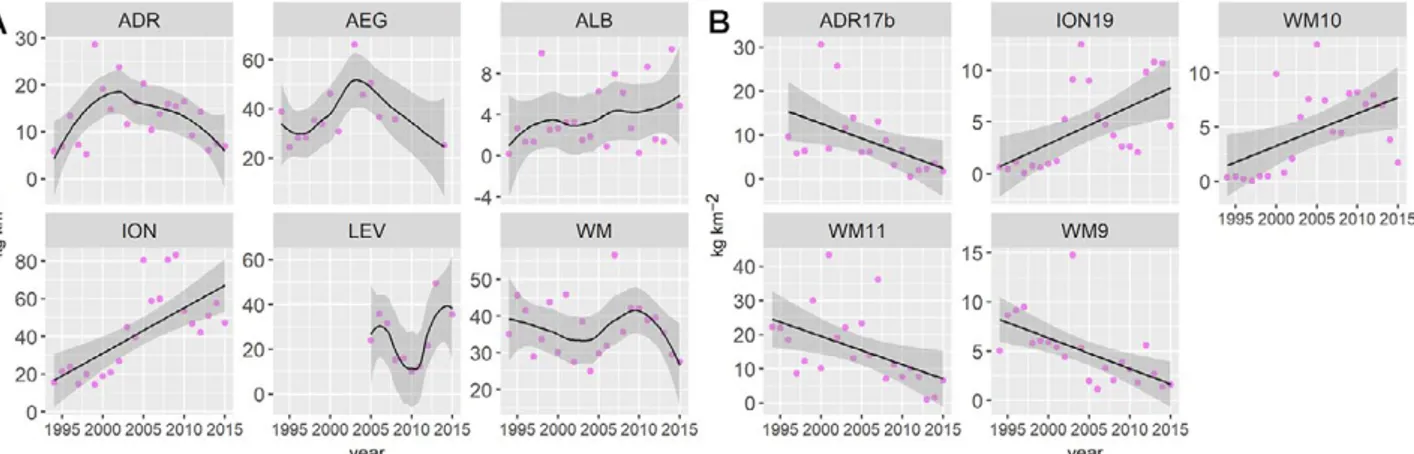
The shelf areas where a significant negative linear trend in BIy was found were the Gulf of Lions (GSAs
7, r2=0.27, p<0.01) and the southern Tyrrhenian Sea
(r2=0.28, p<0.01) while the trend was positive in
northern Spain (GSAs 6, r2=0.30, p<0.05) and south
of Sicily (GSA 16, r2=0.30, p<0.01) (Fig. 4A).
The highest mean BIy values of gurnards on the
continental slope in the last three years of the time series were found in the Gulf of Lions (45.8 kg km–2), Maltese waters (28.3 kg km–2) and the
east-ern Ionian Sea (38.6 kg km–2 in 2004-2008). For the
same period, the lowest relative biomass (BIy <3.0
kg km–2)occurred in the Alboran, western Ionian,
northern Tyrrhenian and Ligurian seas, as well as on the Italian side of GSA 17. Gurnard BIy increased
linearly over time in the Tyrrhenian and Ligurian seas [GSA 9 (r2=0.19, p<0.05) and GSA 10 (r2=0.14,
p<0.05] and in the Ionian Sea [GSA 19 (r2=0.27,
p<0.01) and GSA 20 (r2=0.26, p<0.05]. A linear
decrease occurred in the Balearic Islands (r2=0.44,
p<0.05), eastern Corsica (r2=0.18, p<0.05) and
Sar-dinia (r2=0.29, p<0.05) (Fig. 4B).
Temporal trends in species abundance
Lepidotrigla cavillone
The large-scaled gurnard was mostly distributed on the outer shelf between 36 and 187 m depth. It dis-played an almost linear decrease in relative biomass in the western Mediterranean (r2=0.38, p<0.01) and in the
Aegean ecoregion (r2=0.49, p<0.01), while it increased
in the Ionian ecoregion (r2=0.27, p<0.01) (Fig. 5).
At the GSA level a positive linear trend was found in the south of Sicily (r2=0.27, p<0.01), where there was a
224% increase in BIy in 2013-2015 compared with the
beginning of MEDITS, and in eastern Corsica (GSA 8, +109%: r2=0.22, p<0.05). The trend was significantly
decreasing in the Gulf of Lions (–69%: r2=0.48, p<0.01),
in the southern Tyrrhenian (–75%; r2=0.17, p<0.05) and
northwestern Adriatic seas (–63%: r2=0.18, p<0.05)
(Fig. 5B; Appendix 1). During the period 2013-2015 the highest relative species abundances occurred in Cyprus (26.7 kg km–2), Maltese waters (26.2 kg km–2) and
east-ern Corsica (GSA 8: 23.0 kg km–2). High BI
y was also
found in the eastern Ionian Sea (36 kg km–2) during the
Table 2. – Mean MEDITS biomass index (BIy: kg km–2) of gurnards (all species pooled) on the continental slope (200-800 m) per GSA and year from 1994 to 2015. The proportional rate of change (% change) in BIy was calculated between the first and the last three years of the time
series in the GSAs where a significant linear trend in BIywas found.
GSA 94 95 96 97 98 99 00 01 02 03 04 05 06 07 08 09 10 11 12 13 14 15change% 1 0.0 0.3 0.0 0.1 0.0 0.0 0.0 0.1 0.3 0.1 0.0 0.0 0.2 0.2 0.0 0.0 0.0 0.4 0.2 0.0 0.1 0.3 5 25.9 33.3 35.4 25.5 27.6 23.9 29.7 16.3 15.4 –35.1 6 0.2 0.5 1.1 0.5 0.2 0.0 6.9 3.5 1.0 0.3 0.7 1.4 4.8 2.9 1.7 3.4 0.6 5.1 1.8 1.4 1.9 5.0 7 8.0 58.5 44.8 30.8 27.5 62.8 63.4 44.3 26.4 51.8 39.3 44.4 27.0 31.4 32.0 67.1 46.8 57.3 50.1 19.6 55.4 62.3 8 38.1 41.9 37.7 26.9 37.1 32.6 10.7 37.1 20.3 32.4 28.3 48.6 47.3 26.0 19.2 23.9 23.5 13.5 16.5 25.6 21.2 –46.3 9 0.9 2.0 1.4 1.1 0.9 0.3 1.1 0.6 1.0 1.1 1.8 1.1 1.2 0.7 0.8 6.3 1.8 1.2 4.2 4.2 2.3 1.8 88.0 10 0.7 1.2 1.8 1.7 4.8 1.5 3.5 0.8 1.5 3.1 3.0 6.0 4.4 2.0 4.4 4.9 5.4 3.2 3.7 5.1 2.1 1.5 136.0 11 12.2 9.5 33.0 14.8 19.6 10.5 10.2 22.8 28.4 10.3 4.5 14.3 2.3 12.5 3.2 7.3 4.6 6.2 8.9 4.4 1.8 9.7 –63.9 15 58.6 27.3 1.3 40.3 36.8 36.5 65.7 49.9 24.3 23.9 36.7 16 6.0 1.3 4.8 0.4 1.3 0.7 0.4 2.1 4.0 9.8 2.1 6.9 6.1 10.7 16.8 24.5 4.7 5.8 5.9 4.1 1.1 4.7 17a 0.0 0.1 2.4 2.0 3.7 13.3 3.9 0.4 21.1 13.0 5.8 0.9 1.2 2.5 3.9 1.1 4.4 0.4 0.1 1.1 8.6 2.0 17b 2.2 11.3 1.1 112.4 20.8 1.7 1.4 0.6 1.6 5.7 3.2 0.0 0.4 15.1 0.3 5.9 1.4 6.1 4.7 18 5.7 6.6 9.5 1.2 0.9 29.5 4.8 4.1 14.6 3.4 14.1 7.3 2.6 15.7 8.5 12.3 2.7 2.1 5.1 2.7 4.2 2.9 19 0.0 0.1 0.2 0.3 0.0 0.1 0.3 0.9 0.2 0.5 0.7 0.2 0.9 0.7 0.2 0.3 0.4 2.2 0.4 1.8 0.4 0.9 875.6 20 12.6 0.0 8.1 1.1 7.8 25.0 14.7 24.4 52.1 39.6 39.0 34.0 41.8 15.2 448.3 22 6.7 8.5 10.2 8.1 14.3 21.9 17.9 9.7 28.9 25.8 19.8 16.0 29.9 8.1 23 8.9 0.4 14.0 13.8 24.7 28.8 16.9 28.7 40.5 31.0 27.5 18.1 14.8 9.2 25 17.0 33.9 19.0 11.3 21.5 14.7 9.7 14.3 8.7 30.1
Fig. 4. – All gurnards pooled. GSAs showing a significant linear temporal trend in MEDITS relative biomass index (kg km–2) on the continen-tal shelf (A, 0-200 m) and slope (B, 200-800 m). GSA codes: 10, southern and central Tyrrhenian Sea; 16, south of Sicily; 6, northern Spain; 7, Gulf of Lions; 11, Sardinia; 19, western Ionian Sea; 20, eastern Ionian Sea; 5, Balearic Island; 8, Corsica; 9, Ligurian Sea and northern
period 2004-2008 (Appendix 1). By contrast, very low abundances (BIy <1.5 kg km–2) were found in the
west-ern sector of the Adriatic Sea and in the westwest-ern Ionian and Alboran seas.
Lepidotrigla dieuzeidei
The bulk of the MEDITS catch of spiny gurnard was obtained at depths ranging from 70 to 360 m, with the highest abundances in 2013-2015 found in eastern Corsica (25.7 kg km–2), Sardinia (14.2 kg km–2), the
Balearic Islands (10.0 kg km–2), the eastern Ionian Sea
(9.0 kg km–2) and Malta (8.8 kg km–2, Appendix 2).
The species showed a significant increasing trend in the western Mediterranean (r2=0.21, p<0.05) and Ionian
ecoregions (r2=0.25, p<0.05) during the study period
(Fig. 6A). A significant linear trend was found in Sar-dinia (r2=0.15, p<0.05), the Ionian GSAs 15 (r2=0.30,
p<0.05), 16 (r2=0.23, p<0.05) and 20 (r2=0.34, p<0.05)
and northernern Spain (r2=0.22, p<0.05) (Fig. 6B). The
species was absent from GSAs 19 and 23, with records also lacking in several other GSAs, especially during the first MEDITS period (1994-2000, Appendix 2), possibly due to misidentifications and confusion with the congeneric L. cavillone.
Lepidotrigla spp.
Appendix 3 shows the abundances and trends in the relative biomass of the two Lepidotrigla species com-bined for the 26-360 m depth range, where more than 90% of the positive hauls for the two species were found. The resulting pattern is not very different from the one observed for the large-scaled gurnard, which was more abundant than the spiny gurnard in most of the GSAs. The main differences were a significant increase in the Alboran Sea (+918% in BIy), mostly due to the
occur-rence of the spiny gurnard in the catch of the last three years, and a decrease in the Aegean Sea (–55.1% in BIy). Chelidonichtys cuculus
Red gurnard was mostly distributed between 60 and 270 m, where it achieved the highest relative abundance in the period 2013-2015 in the Balearic Islands (43.8 kg km–2), south of Sicily (19.8 kg km– 2), Malta (13.2 kg km–2) and the Aegean Sea (GSA
22: 11.5 kg km–2, Appendix 4). A positive trend
(r2=0.46, p<0.01) was found in the Ionian
ecore-gion, with a strong increasing trend in the western Ionian Seas (+1039%, r2=0.34, p<0.01) (Fig. 7A
Fig. 5. – Lepidotrigla cavillone. Mean and 95% confidence intervals of the MEDITS relative biomass index (kg km–2) in the Mediterranean ecoregions (A) and geographical sub-areas (GSAs, B) where a significant linear trend was found. GSA codes: 10, southern and central
Tyr-rhenian Sea; 16, south of Sicily; 17a, NW Adriatic Sea; 22, Aegean Sea; 7, Gulf of Lions; 8, eastern Corsica.
Fig. 6. – Lepidotrigla dieuzeidei. Mean and 95% confidence intervals of the MEDITS relative biomass index (kg km–2) in the Mediterranean ecoregions (A) and geographical sub-areas (GSAs, B) where a significant linear trend was found. GSA codes: 11, Sardinia; 15, Malta; 16,
and Appendix 4). In the western Mediterranean, the
BIy fluctuated from 1994 with a contrasted spatial
pattern: a sharply increasing trend in the southern Tyrrhenian (+1102%, r2=0.22, p<0.05) and a
de-creasing trend in the northern Tyrrhenian and Ligu-rian Seas (–75.0%, r2=0.34, p<0.01) and in Sardinia
(–85%, r2=0.21, p<0.05) (Fig. 7). In the Adriatic
Sea the species was much more abundant on the east side, where, however, it declined significantly from the 1990s (–73.7%, r2=0.21, p<0.05) (Fig. 7B,
Appendix 4).
Chelidonichthys obscurus
The longfin gurnard is a shelf species, mostly oc-curring between 20 and 120 m depth. It was absent in the Adriatic and Levantine ecoregions, occurring spo-radically at a very low relative biomass in the Aegean Sea (Fig. 8A). The temporal trend showed a signifi-cant decrease in the western Mediterranean (r2=0.21,
p<0.05, Fig. 8A) where a linear reduction appeared in GSAs 6 (–88%: r2=0.13, p<0.05) and 7 (–96%,
r2=0.21, p<0.05, Fig. 8B). The highest recent
(2013-2015) BIy was found in southern Sicily (1.3 kg km–2),
where, however, the species abundance decreased lin-early (r2=0.14, p<0.05), and in Sardinia (0.9 kg km–2)
(Fig. 8B, Appendix 5). The only area where the species increased linearly through time was the eastern Ionian Sea (r2=0.23, p<0.05, Fig. 8B).
Eutrigla gurnardus
The grey gurnard was more abundant on the continental shelf (30-165 m) of the western Medi-terranean region and particularly in the Gulf of Li-ons. In this area the species was several times more abundant (19.4 kg km–2) than elsewhere. In the other
ecoregions (Fig. 9A), it was found at a very low rela-tive abundance and it was absent from the Alboran and southern Tyrrhenian seas, Crete and Cyprus (Fig. 9B and Appendix 6). A significant and positive linear trend in BIy was found in the Ionian region
(r2=0.48, p<0.01) and specifically in Malta (+58.8%,
r2=0.21, p<0.05) and south of Sicily (+11000%,
r2=0.34, p<0.01, Fig. 9B). Chelidonichthys lucerna
The tub gurnard is also a shelf species, mainly distributed between 15 and 175 m depth. It was sig-nificantly decreasing on the continental shelf of the western Mediterranean (r2=0.48, p<0.01) and
specifi-Fig. 7. – Chelidonichthys cuculus. Mean and 95% confidence intervals of the MEDITS relative biomass index (kg km–2) in the Mediterranean ecoregions (A) and geographical sub-areas (GSAs, B) where a significant linear trend was found. GSA codes: 10, southern and central
Tyr-rhenian Sea; 11, Sardinia; 17b, NE Adriatic Sea; 19, western Ionian Sea; 9, Ligurian Sea and northern TyrTyr-rhenian Sea.
Fig. 8. – Chelidonichthys obscurus. Mean and 95% confidence intervals of the MEDITS relative biomass index (kg km–2) in the Mediterra-nean ecoregions (A) and geographical sub-areas (GSAs, B) where a significant linear trend was found. GSA codes: 16, south of Sicily; 20,
cally in the GSAs 6 (r2=0.13, p<0.05) and 9 (r2=0.22,
p<0.05), while an increasing trend was observed in the GSA 22, in the Aegean Sea (r2=0.41, p<0.01)
(Fig. 10). In the other regions the species fluctuated at low abundance levels without any clear temporal trend (Appendix 7). In 2013-2015 the highest BIy
was obtained on the continental shelf of the Aegean Sea (8.3 kg km–2 in 2014) and the western Ionian Sea
(GSA 19: 2.8 kg km–2, Appendix 7). Trigla lyra
The piper gurnard is typically distributed on the continental slope, with the highest BIyvalues found in
the Gulf of Lions (33.6 kg km–2), Malta (31.1 km–2)
and Balearic waters (23.3 kg km–2) during the period
2013-2015 (Appendix 8). The species showed an in-creasing trend in the western Mediterranean (r2=0.49,
p<0.01) and Ionian (r2=0.50, p<0.01) ecoregions
(Fig. 11A). In the first area, BIy values increased in
the northern Tyrrhenian and Ligurian seas (r2=0.13,
p<0.05), while they decreased in eastern Corsica (r2=0.26, p<0.01). In the Ionian area the species
in-creased in the Strait of Sicily in GSAs 15 (r2=0.25,
p<0.05) and 16 (r2=0.17, p<0.05), and in the western
Ionian Sea (r2=0.17, p<0.05, Fig. 11B).
Chelidonichthys lastoviza
The streaked gurnard was mostly caught between 25 and 120 m depth, with the highest BIy found in
Malta (59.3 kg km–2) and the Balearic Island (34.5 kg
km–2) in 2013-2015. The species was also abundant in
the Aegean Sea in GSA 22 (Appendix 9). It showed an increasing trend in the western Mediterranean (r2=0.29,
p<0.05) and the Ionian ecoregions (r2=0.18, p<0.05,
Fig. 12A). The species showed wide temporal fluctua-tions in BIy, with significant positive linear trends in
GSAs 6 (r2=0.29, p<0.01) and 23 (r2=0.60, p<0.01). A
negative trend was found in GSAs 7 (r2=0.29, p<0.01),
10 (r2=0.45, p<0.01) and 16 (r2=0.23, p<0.05), and on
both the west (r2=0.25, p<0.01) and east side (r2=0.21,
p<0.01) of the northern Adriatic Sea (Fig. 12B).
Peristedion cataphractum
The African armoured searobin was mostly present on the continental slope below 200 m, with 90% of the positive hauls being found between 115 and 550 m depth. It reached by far the highest BIyin Maltese
waters (27.3 kg km–2 in 2013-2015), being generally
more than ten times less abundant in all the other GSAs except GSA 20 in 1994-98 (12.2 kg km–2, Appendix
Fig. 10. – Chelidonichthys lucerna. Mean and 95% confidence intervals of the MEDITS relative biomass index (kg km–2) in the Mediterranean ecoregions (A) and geographical sub-areas (GSAs, B) where a significant linear trend was found. GSA codes: 22, Aegean Sea; 6, northern
Spain; 9, Ligurian Sea and northern Tyrrhenian Sea.
Fig. 9. – Eutrigla gurnardus. Mean and 95% confidence intervals of the MEDITS relative biomass index (kg km–2) in the Mediterranean ecoregions (A) and geographical sub-areas (GSAs, B) where a significant linear trend was found. GSA codes: 15, Malta, 16, south of Sicily.
10). The species showed a linear increasing trend in the Adriatic (r2=0.69, p<0.01), Ionian (r2=0.48, p<0.01)
and Levantine (r2=0.35, p<0.05) ecoregions and a
de-creasing trend in the western Mediterranean (r2=0.47,
p<0.01, Fig. 13A). A positive trend was found in the Adriatic (GSA 17a: r2=0.20, p<0.05 and 18: r2=0.77,
p<0.01), south of Sicily (r2=0.16, p<0.05) and the
west-ern Ionian Sea (r2=0.16, p<0.05), while a significant
linear decrease was observed in Sardinia (r2=0.46,
p<0.01, Fig. 13B). DISCUSSION
This study provides an overview of the status of gurnards in the northern Mediterranean Sea using 22 years of MEDITS bottom trawl survey data. Gurnards Fig. 11. – Trigla lyra. Mean and 95% confidence intervals of the MEDITS relative biomass index (kg km–2) in the Mediterranean ecoregions (A) and geographical sub-areas (GSAs, B) where a significant linear trend was found. GSA codes: 15, Malta; 16, south of Sicily; 19, western
Ionian Sea; 8, eastern Corsica; 9, Ligurian Sea and northern Tyrrhenian Sea.
Fig 12. – Chelidonichthys lastoviza. Mean and 95% confidence intervals of the MEDITS relative biomass index (kg km–2) in the Mediterra-nean ecoregions (A) and geographical sub-areas (GSAs, B) where a significant linear trend was found. GSA codes: 10, southern and central
Tyrrhenian Sea; 16, south of Sicily; 17a, NW Adriatic Sea; 17b, NE Adriatic Sea; 23, Crete; 6, northern Spain; 7, Gulf of Lions.
Fig. 13. – Peristedion cataphractum. Mean and 95% confidence intervals of the MEDITS relative biomass index (kg km–2) in the Mediterra-nean ecoregions (A) and geographical sub-areas (GSAs, B) where a significant linear trend was found. GSA codes: 11, Sardinia; 16, south of
the Mediterranean gurnards have a sub-tropical affin-ity, with only C. cuculus, C. obscurus and E. gurnardus being temperate species (http://www.fishbase.org). In particular, the Ionian and western Mediterranean ecoregions appeared very similar in the structure of the gurnard species guild, with C. cuculus being the most abundant species, followed by five others (L. cavillone,
L. dieuzeidei, T. lyra, C. lastoviza, P. cataphractum or
E. gurnardus) with a similar level of abundance, to-gether accounting for more than 90% of the relative biomass for the examined period. An opposite pattern was observed in the Levantine Sea, where only data for Cyprus are available. Here the k-dominance curve is steep with three species, L. cavillone, C. cuculus and
C. lastoviza dominating the species guild.
The Alboran Sea is featured by the lowest relative biomass of gurnards; the two Lepidotrigla species are the most common gurnards and the grey gurnard is ab-sent. This peculiarity can be related to the influence of Atlantic inputs and the semi-permanent Almería–Oran hydrographic front, which plays a key role in defining the Alboran Sea as a specific fish fauna area within the northern Mediterranean Sea (Gaertner et al. 2005).
In the Adriatic region, the guild is dominated by
L. cavillone, A. cuculus and C. lucerna. Here gurnards were found to be more abundant on the east than on the west side of the basin, probably also due to the eastward ontogenetic migration of the juveniles towards the Croa-tian coasts, as observed for C. cuculus (Vallisneri et al. 2014). Interesting is the absence in this region of the longfin gurnard (C. obscurus), which was also absent in Crete (GSA 23), as reported also by Tsimenides et al. (1992), and in Cyprus (GSA 25). The longfin gurnard also appears rare in the Aegean Sea, where it was not found in a study carried out in the 1970s (Papacon-stantinou 1983). In this region, the four most abundant gurnards, in order of importance, were found to be C.
cuculus, C. lastoviza, C. lucerna and L. cavillone. The species displaying the highest geographical differences are E. gurnardus and P. cataphractum. The first is abundant only in the Gulf of Lions, rare in most of the GSAs and absent in the southern Tyr-rhenian (GSA 10), Crete and Cyprus. The dominance of E. gurnardus on the continental shelf of the Gulf of Lions was already reported by Campillo et al. (1992).
P. cataphractum is consistently more abundant in the Maltese waters than in all the other GSAs.
In terms of overall abundance, the Balearic Islands (GSA 5), Maltese waters (GSA 15), the Gulf of Lions
bility of gurnards is probably high since they live close to the sea bottom, mostly on soft and detrital sediments that are easily exploitable by trawlers. Some local studies support this hypothesis. For example, gurnards were the species showing the highest rate of abundance increase (about 500 fold) on the outer shelf (50-100 m) of northwest Sicily after some years of trawling ban (Pipitone et al. 2000). In the Ionian Sea species like T. lyra, L. dieuzeidei and P. cataphractum were several times more abundant on the poorly exploited continental slope of Greece than on the intensively exploited Italian fishing grounds (D’Onghia et al. 2003). Similarly, in the northern sector of the Strait of Sicily the abundance of gurnards on poorly exploited fishing grounds on the continental slope was several time higher than in the traditionally exploited areas (Gristina et al. 2006). In the same region, Dimech et al. (2008) found higher relative biomass of C. cuculus and
L. cavillone inside the less exploited Fisheries Man-agement Zone (FMZ) of Malta than in the areas outside the FMZ. This evidence supports the hypothesis that the observed geographical differences in gurnard abun-dance may result from the different levels of fishing pressure, with areas less impacted by fishing hosting a higher gurnard biomass. Although more investigation is required on the subject, the results of our study point to a possible future use of gurnards as indicators of the fishing pressure exerted on the ecosystem and, as such, a useful tool for monitoring the fishing impact on the demersal fish communities. A summary of the trend observed since the mid-1990s by species and areas is provided in Figure 14 using a traffic light approach. In the western Mediterranean, a general decrease was found for the shallowest species (C. obscurus, C.
lastoviza and C. lucerna), while a “green” status was more common for the upper slope species (T. lyra and
P. cataphractum). A better situation was observed in the Ionian ecoregion (GSAs 15, 16, 19 and 20), where the “green” status was common for the deep-shelf (e.g.
Lepidotrigla spp., C. cuculus) and upper-slope species. The only significant linear decrease in this region was found for C. obscurus and C. lastoviza in the south of Sicily.
The opposite was observed in the Aegean Sea (GSAs 22-23) and in Cyprus, where the trend was generally positive or stable for the shelf species, with most of the red lights found for deep-shelf and slope gurnard (Fig. 14). A shifting of fishing activities of Greek vessels towards slope resources has recently
been postulated as an effect of the implementation of EC regulation 1967/2006, which bans bottom trawl ac-tivities within 1.5 nautical miles off the coast (Tserpes et al. 2016).
Similarly, deep-water gurnards in Sardinian waters showed the lowest relative biomasses in recent years, with the exception of L. dieuzeidei. P. cataphractum in particular showed a significant linear decrease in abundance across years, in strong contrast with all oth-er ecoregions and GSAs. This temporal pattoth-ern may, besides ecological factors, reflect the modernization of the trawling fishing fleet that took place in the Sardin-ian fisheries (Marongiu et al. 2017), allowing fishing pressure to shift towards deeper habitats such as those inhabited by P. cataphractum.
While there is clear evidence that the excess fishing pressure is reducing the sizes of the gurnard popula-tions in many Mediterranean sectors, there are still important aspects related to the ecology of this guild of species that would be worth exploring in order to understand the factors driving species abundance and distribution. One key feature is related to the habitat preferences of the species. Gurnards seem to prefer de-trital sediments on both the continental shelf and slope.
L. cavillone and C. cuculus off the western coasts of Italy appear more abundant on the detrital bottoms over the continental shelf break (Serena et al. 1990, Colloca
et al. 1997, Damalas et al. 2010). L. diuzeidei was found to be more common on the detrital and muddy bottoms of the shallow part of the upper slope (Voliani et al. 2000), while on the coastal shelf, C. lucerna was concentrated on the coastal and detrital sandy bottoms and C. lastoviza on the coastal detrital sediments (Ser-ena et al. 1990, Ordines et al. 2014). In this study, we found that the areas showing the highest gurnard abun-dances are those characterized by the prevalence or the wide extension of detrital bottoms, such as Malta, the Balearic Islands, the Greek GSAs and the south of Sic-ily, the latter characterized by wide offshore banks (Di Lorenzo et al. 2018). Another important aspect is con-nected with the occurrence of “refugia”, where large spawners of species like C. lucerna can find protection from trawling, as was observed in the western Ionian Sea (D’Onghia et al. 2017).
The rapid ongoing warming of the Mediterranean is another key factor that, in combination with fishing pressure, might explain the species temporal trends observed. The increase in water temperature can be potentially beneficial for sub-tropical species such as the harmoured searobin but have a negative effect on the temperate ones such as E. gurnardus). The overall effect may be a progressive shift in gurnard distribu-tion and abundance as effects of climate forcing. The NAO index, for example, was found to have an indirect effect on triglids by shaping their prey’s availability (López-López et al. 2011). In Portuguese waters the landings of the large-scaled gurnard, a species with a sub-tropical affinity, decreased unexpectedly during the warm years (Teixeira et al. 2014). On the other hand, the congeneric sub-tropical L. dieuzeidei has ex-panded its distribution range in the Atlantic as an effect of the water temperature increase (Punzón et al. 2016).
Future studies on Mediterranean gurnards should focus on the above aspects, in order to understand spe-cifically how fishing pressure, climate forcing and hab-itat suitability interact to determine the trends observed in the present study. Other important aspects that would be worth exploring are related to the compensa-tory effects that may occur within the gurnards guild. The nine species of gurnards inhabiting the Mediter-ranean basin exploit similar trophic niches, preying on the same groups of crustaceans. Therefore, a decrease in the abundance of one or more of these species could be compensated by the increase and the expansion of the more tolerant species, thus avoiding a functional diversity loss in the ecosystem.
REFERENCES
Anonymous. 2017. MEDITS-Handbook. Version n. 9, MEDITS Working Group, 106 pp.
http://www.sibm.it/MEDITS%202011/principaledownload. htm
Bertrand J.A., Gil De Sola L., Papaconstantinou C., et al. 2002. The general specifications of the Medits survey. Sci. Mar. 66: 9-17.
https://doi.org/10.3989/scimar.2002.66s29
Campillo A. 1992. Les pêcheries françaises de Méditerranée. Syn-thèse des connaissances. Rapports Internes de la Direction des Ressources Vivantes de l’Ifremer, RIDRV 92/019 RH Sète: 206 pp.
Cardinale M., Osio G.C., Scarcella G. 2017. Mediterranean Sea: a failure of the European fisheries management system. Front. Fig. 14. – Temporal trend in MEDITS biomass index (BIy: kg
km–2) of Mediterranean gurnards displayed using traffic lights: red, decreasing; green, increasing; orange, stable. Only BIy variation higher than 30% between the initial and final MEDITS period were considered as significant. *, significant linear trend in BIy: (p<0.05).
Colloca F., Carpentieri P., Balestri E., et al. 2010. Food resource partitioning in a Mediterranean demersal fish assemblage: the effect of body size and niche width. Mar. Biol. 157: 565-574.
https://doi.org/10.1007/s00227-009-1342-7
Colloca F., Cardinale M., Maynou F. et al. 2013. Rebuilding Medi-terranean fisheries: a new paradigm for ecological sustainabil-ity. Fish. Fish. 14: 89-109.
https://doi.org/10.1111/j.1467-2979.2011.00453.x
Colloca F., Scarcella G., Libralato S. 2017. Recent trends and impacts of fisheries exploitation on Mediterranean stocks and ecosystems. Front. Mar. Sci. 4: 244.
https://doi.org/10.3389/fmars.2017.00244
Cook R.M., Heath M.R. 2018. Population trends of bycatch spe-cies reflect improving status of target spespe-cies. Fish. Fish. 19: 455-470.
https://doi.org/10.1111/faf.12265
Damalas D., Maravelias C.D., Katsanevakis S., et al. 2010. Sea-sonal abundance of non-commercial demersal fish in the east-ern Mediterranean Sea in relation to hydrographic and sediment characteristics. Est. Coast. Shelf. Sci. 89: 107-118.
https://doi.org/10.1016/j.ecss.2010.06.002
Di Lorenzo M., Sinerchia M., Colloca F. 2018. The North sector of the Strait of Sicily: a priority area for conservation in the Mediterranean Sea. Hydrobiologia 821: 235-253.
https://doi.org/10.1007/s10750-017-3389-7
Dimech M., Camilleri M., Hiddink J.G., et al. 2008. Differences in demersal community structure and biomass size spectra within and outside the Maltese Fishery Management Zone (FMZ). Sci. Mar. 72: 669-682.
https://doi.org/10.3989/scimar.2008.72n4669
D’Onghia G., Mastrototaro F., Matarrese A., et al. 2003. Biodi-versity of the upper slope demersal community in the eastern Mediterranean: preliminary comparison between two areas with and without trawl fishing. J. Northwest. Atl. Fish. Soc. 31: 263.
https://doi.org/10.2960/J.v31.a20
D’Onghia G., Calculli C., Capezzuto F., et al. 2017. Anthropogenic impact in the Santa Maria di Leuca cold-water coral province (Mediterranean Sea): Observations and conservation straits. Deep-Sea Res. II 145: 87-101.
https://doi.org/10.1016/j.dsr2.2016.02.012
Ferrà C., Tassetti A.N., Grati F., et al. 2018. Mapping change in bottom trawling activity in the Mediterranean Sea through AIS data. Mar. Pol. 94: 275-281.
https://doi.org/10.1016/j.marpol.2017.12.013
Gaertner J.C., Bertrand J.A., De Sola L.G., et al. 2005. Large spatial scale variation of demersal fish assemblage structure on the continental shelf of the NW Mediterranean Sea. Mar. Ecol. Prog. Ser. 297: 245-257.
https://doi.org/10.3354/meps297245
Gristina M., Bahri T., Fiorentino F., et al. 2006. Comparison of demersal fish assemblages in three areas of the Strait of Sicily under different trawling pressure. Fish. Res. 81: 60-71.
https://doi.org/10.1016/j.fishres.2006.05.010
Jukic-Peladic S., Vrgoc N., Krstulovic-Sifner S., et al. 2001. Long-term changes in demersal resources of the Adriatic Sea: com-parison between trawl surveys carried out in 1948 and 1998. Fish. Res. 53: 95-104.
https://doi.org/10.1016/S0165-7836(00)00232-0
Kindt R., Coe R. 2005. Tree diversity analysis. A manual and soft-ware for common statistical methods for ecological and biodi-versity studies. World Agroforestry Centre (ICRAF), Nairobi. Labropoulou M., Papaconstantinou C. 2004. Community structure
and diversity of demersal fish assemblages: the role of fishery.
and ontogenetic changes in diet of gurnards (Teleostea: Scor-paeniformes: Triglidae) from the Adriatic Sea. Eur. Zool. J. 84: 356-367.
https://doi.org/10.1080/24750263.2017.1335357
Morte M.S., Redon M.J., Sanz-Brau A. 1997. Trophic relationships between two gurnards Trigla lucerna and Aspitrigla obscura from the western Mediterranean. J. Mar. Biol. Ass. U.K. 77: 527-537.
https://doi.org/10.1017/S0025315400071848
Ordines F., Farriols M.T., Lleonart J., et al. 2014. Biology and population dynamics of by-catch fish species of the bottom trawl fishery in the western Mediterranean. Medit. Mar. Sci. 15: 613-625.
https://doi.org/10.12681/mms.812
Papaconstantinou C. 1981. Age and growth of piper, Trigla lyra, in Saronikos Gulf (Greece). Cybium 5: 73-87.
Papaconstantinou C. 1983. Observations on the ecology of gurnards (Pisces: Triglidae) in the Greek Seas. Cybium 7: 71-88. Papaconstantinou C. 1984. Age and growth of the yellow gurnard
(Trigla lucerna L. 1758) from the Thermaikos Gulf (Greece) with some comments on its biology. Fish. Res. 2: 243-255.
https://doi.org/10.1016/0165-7836(84)90028-6
Pipitone C., Badalamenti F., D’Anna G., et al. 2000. Fish biomass increase after a four-year trawl ban in the Gulf of Castellam-mare (NW Sicily, Mediterranean Sea). Fish. Res. 48: 23-30.
https://doi.org/10.1016/S0165-7836(00)00114-4
Punzón A., Serrano A., Sánchez F., et al. 2016. Response of a tem-perate demersal fish community to global warming. J. Mar. Sys. 161: 1-10.
https://doi.org/10.1016/j.jmarsys.2016.05.001
Richards W.J., Jones D.L. 2002. Preliminary classification of the gurnards (Triglidae: Scorpaeniformes). N. Z. J. Mar. Freshw. Res. 53: 274-282.
https://doi.org/10.1071/MF01128
Serena F., Baino R., Voliani A. 1990. Distribuzione dei Triglidi (Osteichthyes, Scorpaeniformes) nell’Alto Tirreno. Oebalia Suppl. XVI: 269-278.
Spalding M.D., Fox H.E., Allen G.R., et al. 2007. Marine Ecore-gions of the World: a bioregionalization of coast and shelf areas. BioScience 57: 573-583.
https://doi.org/10.1641/B570707
Terrats A., Petrakis G., Papaconstantinou C. 2000. Feeding habits of Aspitrigla cuculus (L., 1758) (red gurnard), Lepidotrigla
cavillone (Lac., 1802) (large scale gurnard) and Trigloporus
lastoviza (Brunn., 1768) (rock gurnard) around Cyclades and Dodecanese Islands (E. Mediterranean). Medit. Mar. Sci. 1: 91-104.
https://doi.org/10.12681/mms.280
Teixeira C.M., Gamito R., Leitão F., et al. 2014. Trends in landings of fish species potentially affected by climate change in Portu-guese fisheries. Reg. Environ. Change 14: 657-669.
https://doi.org/10.1007/s10113-013-0524-5
Tserpes G., Nikolioudakis N., Maravelias C., et al. 2016. Viability and management targets of Mediterranean demersal fisheries: the case of the Aegean Sea. PloS ONE 11: e0168694.
https://doi.org/10.1371/journal.pone.0168694
Tsimenides N., Machias A., Kallioniotis A. 1992. Distribution pat-terns of Triglids (Pisces: Triglidae) on the Cretan shelf (Greece), and their interspecific associations. Fish. Res. 15: 83-103.
https://doi.org/10.1016/0165-7836(92)90006-F
Vallisneri M., Stagioni M., Montanini S., et al. 2011. Body size, sexual maturity and diet in Chelidonichthys lucerna (Osteich-thyes: Triglidae) from the Adriatic Sea, north eastern
Mediter-ranean. Acta Adriat. 51: 141-148.
Vallisneri M., Montanini S., Stagioni M. 2012. Size at maturity of triglid fishes in the Adriatic Sea, northeastern Mediterranean. J. Appl. Ichthyol. 28: 123-125.
https://doi.org/10.1111/j.1439-0426.2011.01777.x
Vallisneri M., Tommasini S., Stagioni M., et al. 2014. Distribution and some biological parameters of the red gurnard
Chelidonich-thys cuculus (Actinopterygii, Scorpaeniformes, Triglidae) in the north-central Adriatic sea. Acta Ichthyol. Piscat. 44: 173-180.
https://doi.org/10.3750/AIP2014.44.3.01
Voliani A., Mannini P., Auteri R. 2000. Distribuzione e biologia di Lepidotrigla cavillone (Lacepedè) e L. dieuzeidei (Auduin in Blanc e Hureau) nell’Arcipelago Toscano. Biol. Mar. Medit. 7: 844-849.
APPENDICES
Appendix 1. – Lepidotrigla cavillone. Mean MEDITS biomass index (BIy: kg km–2) per GSA and year from 1994 to 2015 in the 36-187 m
depth range where 90% of positive hauls occurred. The proportional rate of change (% change) in BIy was calculated between the first and the last three years of the time series in the GSAs where a significant linear trend in BIywas found.
GSA 94 95 96 97 98 99 00 01 02 03 04 05 06 07 08 09 10 11 12 13 14 15change% 1 0.7 0.0 0.3 0.0 5.4 1.9 0.2 2.0 1.7 0.7 1.2 3.6 3.0 7.3 4.4 1.8 0.3 9.2 0.8 0.4 1.7 1.1 5 21.8 8.0 13.3 16.1 13.4 13.2 9.1 13.4 10.2 6 5.1 7.2 2.3 3.4 3.3 2.8 2.1 2.3 1.7 1.4 3.5 3.6 5.7 5.6 1.0 3.2 1.6 2.5 2.0 3.9 4.0 6.0 7 32.4 35.2 44.0 16.0 23.3 51.2 15.7 23.0 18.4 19.3 10.3 7.5 8.3 13.0 18.8 11.4 9.1 8.4 9.1 15.5 8.4 10.6 –69.1 8 12.7 20.3 0.0 18.8 9.5 22.0 10.3 15.4 9.8 8.0 16.2 13.2 10.6 24.5 29.1 11.3 27.3 31.7 30.0 10.8 28.3 109.3 9 6.4 3.8 3.9 3.8 3.8 4.8 4.8 3.2 4.7 1.8 3.4 2.8 2.9 3.6 4.4 4.5 5.5 3.6 5.5 3.2 4.0 1.6 10 7.9 16.2 15.8 5.9 16.9 11.2 11.5 1.2 11.7 5.5 1.3 6.1 5.7 8.6 3.5 9.8 9.0 10.6 11.7 4.4 3.7 1.8 –75.1 11 19.7 6.8 9.0 11.6 14.9 11.6 15.3 29.4 2.3 6.1 9.7 12.0 10.4 29.1 8.8 14.8 15.8 7.3 9.8 4.2 3.0 6.7 15 14 41.5 39.7 44.0 33.3 16.0 35.8 20.4 25.8 26.3 26.6 16 5.6 4.7 3.0 7.1 5.5 6.1 8.4 4.9 15.5 2.1 11.2 26.0 17.6 14.5 23.0 21.0 25.9 10.9 8.2 14.2 20.0 8.8 224.0 17a 0.1 3.2 3.8 3.1 0.8 2.0 2.3 0.9 1.2 1.1 1.3 1.1 0.8 0.9 1.4 1.2 2.0 0.9 1.0 0.9 1.0 0.8 –62.9 17b 12.6 6.3 4.9 7.6 5.6 8.2 4.2 13.3 14.0 7.8 5.7 15.8 18.7 12.4 7.0 12.8 6.0 4.6 8.4 18 1.2 1.4 1.3 1.3 1.7 4.6 3.7 11.1 13.7 2.3 3.6 10.8 2.8 1.3 2.2 3.3 6.9 5.1 6.0 0.7 3.1 0.5 19 9.9 0.6 0.5 0.0 0.2 0.0 0.1 0.2 5.3 1.0 3.7 1.1 1.4 0.4 1.8 0.5 0.3 0.7 2.0 1.3 2.6 1.3 20 8.9 10.5 27.0 11.3 23.0 15.6 18.2 16.0 15.5 22.7 69.9 25.8 25.3 7.8 22 11.2 14.5 13.3 11.5 12.4 13.1 17.2 7.3 9.8 8.1 13.3 3.5 9.5 3.6 23 16.7 35.9 24.8 15.9 27.2 42.3 5.4 20.0 29.8 19.6 7.2 8.1 26.5 0.0 25 8.8 10.3 11.8 6.9 9.8 4.5 7.3 12.1 35.0 18.4
Appendix 2. – Lepidotrigla dieuzeidei. Mean MEDITS biomass index (BIy: kg km–2) per GSA and year from 1994 to 2015 in the 70-360 m
depth range where 90% of positive hauls occurred. The proportional rate of change (% change) in BIy was calculated between the first and the last three years of the time series in the GSAs where a significant linear trend in BIywas found.
GSA 94 95 96 97 98 99 00 01 02 03 04 05 06 07 08 09 10 11 12 13 14 15change% 1 0.0 0.0 0.0 0.0 0.0 0.0 0.0 0.0 0.0 0.0 0.0 0.0 0.0 0.2 0.1 0.0 0.0 0.0 0.4 0.3 3.5 0.8 + 5 3.8 3.7 12.4 11.7 14.9 19.3 8.6 11.8 9.2 6 0.0 0.0 0.01 0.0 0.0 0.0 0.0 0.0 0.0 0.0 0.0 0.1 0.0 0.0 0.0 0.0 0.0 0.0 0.0 0.0 0.5 0.6 10046.4 7 0.0 0.2 0.6 1.1 0.5 2.5 2.7 1.1 1.4 0.8 0.8 0.1 0.8 2.4 0.7 0.1 0.1 1.3 1.0 1.2 1.3 0.8 8 21.8 20.3 34.5 6.8 0.1 40.5 5.3 50.2 18.2 15.1 25.8 34.3 48.4 20.8 0.7 31.2 29.4 14.3 19.3 34.1 23.8 9 0.3 1.2 3.2 3.3 6.5 3.1 2.6 0.3 1.1 14.1 4.2 3.6 1.9 1.4 2.4 5.0 5.7 4.3 2.1 1.2 1.5 3.7 10 0.0 0.0 0.0 0.0 0.0 0.0 0.0 0.0 0.0 0.0 0.0 1.5 0.0 0.0 0.0 1.1 0.8 0.7 0.5 0.6 0.7 0.5 + 11 2.6 4.7 7.5 2.9 16.8 20.7 4.8 18.1 10.0 11.8 2.5 9.2 11.4 14.3 2.6 18.3 10.3 22.8 19.9 10.8 8.1 23.7 187.2 15 0.0 0.0 2.8 6.8 12.7 5.4 16.3 10.3 9.5 10.4 6.4 843.1 16 0.0 0.0 0.05 0.0 0.0 0.0 0.0 0.0 0.0 7.6 2.8 0.0 3.4 5.5 25.3 14.3 5.7 5.1 5.9 8.7 4.6 4.1 35838.2 17a 0.0 0.0 0.0 0.0 0.9 0.2 0.2 0.0 0.5 0.0 0.1 0.2 0.0 0.0 0.9 0.3 0.2 0.1 0.4 0.1 0.3 0.1 + 17b 0.3 0.0 0.0 0.8 0.0 0.4 0.7 2.5 1.3 0.2 0.7 1.3 0.1 1.5 0.4 0.6 0.2 0.2 0.4 18 0.0 0.0 0.0 0.0 0.0 0.05 0.0 0.0 0.0 0.0 0.0 0.3 0.0 0.0 0.1 9.5 1.1 0.9 1.7 2.0 0.6 0.0 19 0.0 0.0 0.0 0.0 0.0 0.0 0.0 0.0 0.0 0.0 0.0 0.0 0.0 0.0 0.0 0.0 0.0 0.0 0.0 0.0 0.0 0.0 20 0.0 0.0 4.6 0.9 3.1 4.1 5.1 11.5 29.6 19.6 25.6 25.4 19.4 9.0 485.5 22 1.3 0.0 4.7 1.4 0.4 0.6 0.7 0.5 3.1 6.1 3.4 2.6 3.4 0.7 23 0.1 0.0 0.2 0.0 0.0 0.0 0.0 0.0 0.0 0.3 0.0 0.0 0.0 0.0 25 1.0 1.2 1.6 0.0 0.1 0.1 0.0 0.0 0.0 0.6
Appendix 4. – Chelidonichthys cuculus. Mean MEDITS biomass index (BIy: kg km–2) per GSA and year from 1994 to 2015 in the 60-270 m
depth range where 90% of positive hauls occurred. The proportional rate of change (% change) in BIy was calculated between the first and the last three years of the time series in the GSAs where a significant linear trend in BIywas found.
GSA 94 95 96 97 98 99 00 01 02 03 04 05 06 07 08 09 10 11 12 13 14 15change% 1 0.1 0.0 0.3 1.1 0.9 0.3 0.7 0.1 0.4 0.4 0.2 0.6 0.5 1.0 0.1 0.0 0.0 0.1 0.0 0.1 1.4 1.7 5 70.5 33.3 40.6 70.1 62.8 49.8 39.2 68.7 23.5 6 2.0 3.1 0.9 0.6 7.6 3.0 2.3 7.1 0.9 1.9 2.1 4.5 8.2 9.5 1.0 1.8 1.6 3.5 3.7 3.6 4.3 4.6 7 8.3 11.2 12.4 7.9 8.5 18.9 9.6 16.0 6.2 6.4 4.5 4.9 8.4 11.8 8.4 3.9 7.7 6.3 8.4 13.3 4.6 4.4 8 8.1 10.4 20.1 6.4 45.8 19.3 10.6 19.7 13.9 18.1 10.2 11.3 31.7 18.2 13.5 11.6 8.1 12.4 17.1 5.8 9.4 9 5.1 8.7 9.1 9.5 5.8 6.1 5.9 5.4 4.4 14.8 5.3 2.0 1.2 3.3 2.1 3.9 3.1 1.8 5.6 2.7 1.4 1.6 –75.0 10 0.4 0.4 0.2 0.0 0.5 0.5 9.9 0.8 2.1 5.9 7.6 12.6 7.5 4.6 4.5 8.1 8.2 7.2 7.9 7.0 3.8 1.7 1102.0 11 22.3 22.0 18.4 8.6 12.3 30.0 10.1 43.4 19.2 22.0 13.1 23.4 14.0 36.3 7.1 11.2 7.7 10.1 7.6 1.0 1.6 6.6 –85.3 15 8.1 11.4 13.3 17.3 14.0 11.2 11.6 13.1 8.8 17.3 13.4 16 7.9 33.0 17.3 3.9 3.7 1.6 4.0 4.0 16.2 15.5 20.6 29.8 32.4 33.6 32.3 25.0 30.5 12.2 14.7 18.5 22.9 17.9 17a 0.1 0.6 0.5 0.6 0.2 1.9 2.6 0.2 2.3 0.8 0.5 0.6 0.3 1.7 1.2 0.5 0.4 1.8 0.9 0.4 1.2 0.5 17b 9.6 5.8 6.3 30.6 6.9 25.7 11.7 13.9 6.1 6.2 13.1 8.7 3.2 6.7 0.6 2.1 2.2 3.6 1.8 –73.7 18 5.7 8.0 10.3 0.8 1.9 38.7 8.4 13.0 12.1 5.4 10.5 20.3 8.0 13.2 12.2 17.6 14.2 10.1 19.3 7.2 7.9 2.8 19 0.7 0.5 1.2 0.1 0.8 0.6 1.0 1.3 5.3 9.1 12.5 9.0 5.6 4.7 3.7 2.6 2.6 2.1 9.8 10.8 10.7 4.6 1039.8 20 0.0 2.1 14.3 4.7 10.7 3.1 4.6 13.5 17.9 9.5 18.7 15.7 17.9 7.1 22 16.0 8.4 7.9 13.4 18.1 11.4 28.7 19.8 40.7 28.9 32.1 22.4 21.7 11.5 23 1.2 0.8 0.1 6.2 14.1 5.0 3.1 5.4 33.7 9.0 13.4 12.4 16.0 6.0 25 10.7 19.4 11.7 4.8 1.7 3.0 1.6 3.2 3.1 7.8
Appendix 5. – Chelidonichthys obscurus. Mean MEDITS biomass index (BIy: kg km–2) per GSA and year from 1994 to 2015 in the 20-120 m
depth range where 90% of positive hauls occurred. The proportional rate of change (% change) in BIy was calculated between the first and the last three years of the time series in the GSAs where a significant linear trend in BIywas found.
GSA 94 95 96 97 98 99 00 01 02 03 04 05 06 07 08 09 10 11 12 13 14 15change% 1 0.0 0.0 0.0 0.4 0.0 0.0 0.1 0.3 0.4 0.0 0.0 0.0 1.5 0.5 0.2 0.0 0.0 0.6 0.0 0.9 0.9 0.1 5 0.5 0.0 0.0 0.0 0.0 0.0 0.0 0.0 0.0 6 0.1 1.8 0.3 0.1 0.1 0.0 0.6 0.2 0.2 0.0 0.1 0.2 0.3 0.2 0.0 0.1 0.0 0.1 0.1 0.1 0.1 0.1 –87.9 7 1.2 6.7 2.0 0.4 0.1 0.1 0.1 0.0 3.1 0.4 0.1 0.1 0.1 0.7 0.4 0.2 0.0 0.0 0.1 0.3 0.0 0.0 –96.1 8 0.0 0.2 0.0 0.0 0.0 0.0 0.0 0.0 0.0 0.0 0.0 0.0 0.0 0.0 0.0 0.0 0.3 0.1 0.0 0.0 0.0 9 0.7 0.3 0.5 0.2 0.2 0.2 0.3 0.2 0.3 0.1 1.0 0.4 0.0 2.1 0.0 0.0 0.1 0.0 0.8 0.1 0.1 0.3 10 0.0 0.0 0.0 0.0 0.0 0.1 0.0 0.2 0.1 0.1 0.1 0.4 0.1 0.2 0.0 0.2 0.2 0.2 0.0 0.2 0.0 0.0 11 1.5 0.3 0.5 2.3 0.9 1.0 1.2 4.0 3.0 0.8 0.2 1.9 0.6 3.5 0.0 1.4 1.3 1.2 1.6 1.5 0.9 0.3 15 0.0 0.7 0.2 0.5 0.0 0.0 0.0 0.0 0.3 0.0 1.0 16 1.2 5.2 7.8 14.3 3.2 3.3 9.2 2.0 2.5 5.3 8.8 1.7 1.6 3.1 4.4 3.0 4.7 6.3 1.2 2.5 0.2 1.1 –64.6 17a 0.0 0.0 0.0 0.0 0.0 0.0 0.0 0.0 0.0 0.0 0.0 0.0 0.0 0.0 0.0 0.0 0.0 0.0 0.0 0.0 0.0 0.0 17b 0.0 0.0 0.0 0.0 0.0 0.0 0.0 0.0 0.0 0.0 0.0 0.0 0.0 0.0 0.0 0.0 0.0 0.0 0.0 18 0.0 0.0 0.0 0.0 0.0 0.0 0.0 0.0 0.0 0.0 0.0 0.0 0.0 0.0 0.0 0.0 0.0 0.0 0.0 0.0 0.0 0.0 19 0.0 0.0 0.0 0.0 0.0 0.0 0.0 0.1 0.0 0.0 0.02 0.1 0.1 0.3 0.1 0.0 0.0 0.3 0.1 0.0 0.0 0.0 20 0.0 0.0 0.0 0.0 0.1 0.0 0.0 0.0 0.0 0.0 0.2 0.0 0.3 0.1 572.7 22 0.0 0.04 0.0 0.0 0.0 0.0 0.1 0.0 0.0 0.0 0.0 0.0 0.0 0.0 23 0.0 0.0 0.0 0.0 0.0 0.0 0.0 0.0 0.0 0.0 0.0 0.0 0.0 0.0 25 0.0 0.0 0.0 0.0 0.0 0.0 0.0 0.0 0.0 0.0 17b 11.3 5.8 4.6 8.1 4.8 7.8 4.2 13.9 13.6 7.2 5.5 15.3 16.7 12.4 6.4 11.4 4.9 3.7 7.1 18 0.9 1.1 1.2 1.2 1.7 5.2 3.4 10.5 13.0 2.3 3.5 10.3 2.6 1.2 2.1 3.6 7.1 5.5 5.9 2.3 3.4 0.5 19 8.9 0.6 0.4 0.0 0.1 0.0 0.1 0.2 3.5 0.6 2.7 0.8 1.0 0.3 1.3 0.4 0.2 0.5 1.3 0.9 1.9 0.9 20 6.4 8.5 35.6 13.1 24.2 16.4 18.1 24.3 27.7 30.3 82.4 46.9 45.2 10.9 22 10.0 10.6 12.4 9.9 10.4 10.8 14.1 6.6 9.6 10.4 18.4 5.0 31.3 4.9 –55.1 23 9.2 25.4 22.3 11.5 28.5 31.6 5.2 20.7 32.0 18.1 6.5 8.0 21.9 0.0 25 8.8 10.1 11.5 6.3 8.9 4.2 6.6 11.1 31.3 16.8
Appendix 6. – Eutrigla gurnardus. Mean MEDITS biomass index (BIy: kg km–2) per GSA and year from 1994 to 2015 in the 30-165 m depth
range where 90% of positive hauls occurred. The proportional rate of change (% change) in BIy was calculated between the first and the last three years of the time series in the GSAs where a significant linear trend in BIywas found.
GSA 94 95 96 97 98 99 00 01 02 03 04 05 06 07 08 09 10 11 12 13 14 15change% 1 0.0 0.0 0.0 0.0 0.0 0.0 0.0 0.0 0.0 0.0 0.0 0.0 0.0 0.0 0.0 0.0 0.0 0.0 0.0 0.0 0.0 0.0 5 0.0 0.0 0.0 0.2 0.2 0.0 0.0 0.0 0.1 6 0.3 3.8 0.3 0.9 0.0 0.1 3.1 0.2 0.2 0.2 0.3 1.2 1.6 0.1 0.1 0.3 0.1 0.1 0.2 0.7 1.6 5.4 7 46.2108.1 53.0 22.6 16.9 22.2 35.9 38.5 44.4 27.9 28.5 22.0 39.4 31.6 53.3 47.4 36.5 25.5 37.2 35.9 11.7 10.5 8 0.0 0.0 0.0 0.0 0.5 0.0 0.0 0.0 0.0 0.0 0.0 0.0 0.0 0.0 0.0 0.0 0.0 0.0 0.0 0.0 0.2 9 0.3 0.3 0.1 0.2 0.0 0.1 0.1 0.1 0.3 0.1 0.1 0.05 0.02 0.6 0.05 0.3 0.7 0.4 0.1 0.1 0.3 0.1 10 0.0 0.0 0.0 0.0 0.0 0.0 0.0 0.0 0.0 0.0 0.0 0.0 0.0 0.0 0.0 0.0 0.0 0.0 0.0 0.0 0.0 0.0 11 0.0 0.2 0.1 0.2 0.03 0.3 0.5 1.2 0.0 0.5 0.1 0.6 0.2 1.2 0.1 0.3 0.3 0.2 0.8 0.6 0.7 0.3 15 0.0 3.5 3.8 3.4 1.6 1.7 4.0 4.9 2.8 5.0 3.8 58.8 16 0.0 0.0 0.0 0.04 0.0 0.0 0.1 0.0 0.04 0.0 0.3 0.01 0.2 0.2 0.02 0.01 0.1 0.04 0.2 0.1 0.3 0.611008.1 17a 1.1 0.5 0.6 0.3 0.3 1.6 1.8 0.7 3.5 3.0 2.6 2.2 1.7 0.9 1.4 0.4 0.5 0.6 0.4 0.3 0.5 0.6 17b 4.0 1.0 1.0 2.4 0.9 7.4 6.8 5.7 5.7 2.9 1.6 2.8 2.0 1.0 0.6 1.1 1.4 0.4 9.6 18 0.1 0.3 0.1 0.04 0.0 0.2 0.3 0.4 2.3 0.4 0.7 0.3 0.2 0.1 0.4 0.5 0.3 0.2 0.2 0.2 0.1 0.03 19 0.0 0.2 0.03 0.03 0.1 0.2 0.1 0.01 0.9 0.4 1.3 0.4 0.5 0.0 0.6 0.1 0.1 0.1 0.1 0.1 0.2 0.01 20 0.2 0.0 0.8 0.0 0.1 0.2 0.7 2.4 0.4 3.9 1.0 1.3 1.2 0.8 22 1.4 0.7 1.1 0.4 0.9 2.1 0.7 0.9 4.4 2.1 3.2 2.8 0.6 1.4 23 0.0 0.0 0.0 0.0 0.0 0.0 0.0 0.0 0.0 0.0 0.0 0.0 0.0 0.0 25 0.0 0.0 0.0 0.0 0.0 0.2 0.0 0.01 0.0 0.0
Appendix 7. – Chelidonichthys lucerna. Mean MEDITS biomass index (BIy: kg km–2) per GSA and year from 1994 to 2015 in the 15-175 m
depth range where 90% of positive hauls occurred. The proportional rate of change (% change) in BIy was calculated between the first and the last three years of the time series in the GSAs where a significant linear trend in BIywas found.
GSA 94 95 96 97 98 99 00 01 02 03 04 05 06 07 08 09 10 11 12 13 14 15change% 1 0.6 0.0 0.0 0.0 1.4 0.6 1.9 1.9 0.5 0.2 0.0 0.0 0.6 0.0 0.0 1.7 0.0 0.5 0.0 0.5 0.0 0.0 5 0.0 0.0 0.0 0.1 0.0 0.0 0.0 0.7 0.0 6 0.6 0.0 0.4 0.5 0.5 0.4 1.2 0.6 0.5 1.3 1.7 0.1 0.5 0.2 0.0 0.1 0.0 0.01 0.1 0.1 0.0 0.05 –88.5 7 0.2 0.2 0.1 0.3 0.1 1.2 0.4 0.1 0.4 0.2 0.0 0.4 0.4 0.3 0.6 0.4 0.2 0.3 0.1 0.3 0.2 0.0 8 0.0 0.0 0.6 0.0 0.0 2.5 0.0 3.3 0.2 0.8 1.3 0.0 0.0 0.0 0.0 3.7 0.0 0.4 0.4 0.5 0.0 9 0.8 1.5 1.8 1.3 1.3 1.4 0.9 0.4 1.6 1.8 1.5 0.8 0.6 1.3 0.4 1.1 0.2 0.4 0.8 0.6 0.4 1.3 –44.5 10 1.6 0.8 0.3 2.0 0.8 0.5 0.4 1.6 1.4 2.1 0.3 1.2 2.5 1.5 0.7 2.0 0.4 0.9 0.8 1.5 1.4 0.6 11 1.4 0.5 1.6 0.5 0.6 0.8 0.3 0.5 0.6 0.4 0.2 0.6 1.1 2.5 0.0 0.2 0.3 0.4 0.6 0.2 0.1 0.1 15 0.0 0.0 0.0 0.0 0.4 0.0 0.0 0.2 0.0 0.0 0.0 16 1.0 0.5 1.8 1.8 2.4 0.5 2.9 0.5 1.0 3.3 1.3 1.8 0.8 1.1 1.2 1.7 1.4 0.4 1.0 2.0 0.8 1.4 17a 0.3 0.03 0.6 0.4 0.4 13.5 3.8 1.3 8.3 1.6 2.4 4.3 4.6 1.2 0.9 0.3 0.7 1.0 0.7 1.2 2.4 2.3 17b 0.1 0.1 0.0 0.8 0.3 0.5 0.6 0.4 0.5 0.7 0.5 0.6 2.6 0.4 0.0 0.5 0.7 0.2 0.7 18 0.1 0.2 1.1 1.2 0.9 9.2 1.0 0.9 3.9 1.9 0.3 1.2 1.6 3.4 4.4 0.9 0.9 0.7 1.1 1.8 1.0 0.5 19 0.5 2.9 0.9 0.1 3.1 2.0 0.5 1.0 15.1 1.0 8.6 3.0 1.2 1.0 4.7 1.3 2.2 2.9 4.0 3.3 1.7 1.7 20 0.0 0.1 0.7 0.0 0.5 1.4 1.1 0.8 5.9 0.0 0.0 0.1 0.1 0.9 22 0.9 0.3 1.0 1.2 0.7 0.9 0.9 0.7 2.5 1.5 1.8 1.0 1.2 8.3 999.3 23 5.3 0.8 1.4 1.1 12.8 3.9 0.6 3.8 9.6 3.2 3.0 1.5 3.0 0.7 25 0.4 0.3 0.2 0.1 0.2 0.1 0.2 0.2 2.3 0.2
Appendix 8. – Trigla lyra. Mean MEDITS biomass index (BIy: kg km–2) per GSA and year from 1994 to 2015 in the 90-445 m depth range
where 90% of positive hauls occurred. The proportional rate of change (% change) in BIy was calculated between the first and the last three years of the time series in the GSAs where a significant linear trend in BIywas found.
GSA 94 95 96 97 98 99 00 01 02 03 04 05 06 07 08 09 10 11 12 13 14 15change% 1 0 0 0.18 0.1 0 0 0 0 0.07 0 0 0.01 0.2 0.23 0 0.13 0 0.08 0 0 0.05 0.25 5 17.5 27 29.5 21.5 35.9 22.9 24.2 29.1 16.6 6 0.77 2.15 1.86 2.11 5.02 0.82 8.81 1.49 0.8 0.89 1.19 1.44 4.01 2.62 0.45 3.74 0.61 5.32 2.46 1.95 3.76 2.19 7 6.07 34 20.5 14.6 9.41 27.9 37.4 30.5 19.5 36.9 18.6 29.6 16.6 16.8 12.7 31.8 20.2 29.9 26.4 31.6 36.5 32.7 8 7.94 34.4 17.5 30 8.81 4.88 5.5 0.21 4.67 9.59 6.71 9.18 6.19 12.2 6.05 5.39 2 2.15 4.28 7.17 3.92 –74.3 9 0.94 2.22 1.28 0.92 0.77 0.55 0.91 0.48 0.82 1.35 1.82 0.93 1.15 0.87 2.14 5.12 2.14 1.24 0.7 5.7 2.25 1.37 110.1 10 0.17 0.26 0.11 0.15 4.81 0.3 0.2 0.44 0.2 0.9 1 0.75 0.46 1.72 0.51 1.32 2.7 0.85 0.91 0.92 0.82 0.13 11 3.39 1.93 4.63 3.78 3.08 1.3 1.09 2.83 2.67 3.24 4.58 5.62 1.77 5.19 2.79 1.92 1.9 2.85 1.84 1.22 1.18 2.27 15 3.25 14.2 4.94 10.6 17.7 12.1 59.6 13.7 27.4 44.5 21.3 317.1 16 0.08 0.23 0 0.02 0.57 0.53 0.32 2.34 0.72 1.58 1.25 3.02 2.96 7.14 5.5 35.6 4.66 4.98 5.67 7.45 6.08 6.59 6443.5 17a 0 0.12 0.37 0.2 0.08 0.32 0.11 0.09 0.21 0.23 0.39 0.15 0.31 0.26 0.33 0.12 0.1 0.08 0.05 0.04 0.18 0.09 17b 0.97 0.89 0.2 0.43 0.73 0.59 0.66 0.32 0.22 0.47 0.96 1.03 2.87 0.3 0.13 0.1 0.18 0.19 1.46 18 0.23 0.05 0.48 0.39 0.06 0.25 0.38 0.6 0.68 0.6 1.89 0.68 0.46 0.57 1.55 1.26 1.64 0.41 0.95 0.25 0.36 0.1 19 0.21 0.41 0.08 0.3 0 0.15 0.02 0.11 0.32 0.07 0.27 0.21 0.79 0.48 0.28 0.21 0.27 0.32 3.01 1.51 0.37 0.55 248.1 20 2.08 0 0.13 0.74 0.62 1.3 0.74 1.43 0.6 2.77 6.2 2.54 3.05 1.52 22 9.08 4.55 3.4 1.39 6.47 15.5 6.92 2.16 11.1 6.62 2.76 4.26 1.98 1.54 23 7.13 0 6.98 0 0 0 0.49 0 0 0 0 0 0 0 25 0 0.11 0.53 0.06 0.53 0 0 0 0 0
17b 4.4 3.8 2.8 4.4 6.2 5.9 5.6 3.3 3.4 1.8 3.5 4.0 3.8 2.3 1.3 3.7 4.0 1.8 2.3 –28.3 18 0.2 0.0 0.1 0.0 0.0 0.3 0.1 0.3 0.8 0.2 0.2 0.5 0.1 0.0 0.0 0.5 1.4 0.9 1.1 0.2 0.2 0.1 19 0.3 0.1 0.3 0.0 0.0 0.2 0.6 0.1 6.7 1.9 8.6 0.4 0.7 0.1 0.4 0.1 0.8 0.9 0.9 0.4 0.4 0.7 20 0.9 0.0 25.6 19.5 1.2 0.8 1.7 1.9 2.4 2.6 4.8 5.0 5.4 5.4 22 5.1 16.1 14.2 7.1 5.1 11.2 11.2 7.3 25.4 12.1 18.5 9.9 20.7 12.8 23 0.7 0.0 1.8 0.0 0.0 3.7 8.2 1.8 7.9 3.5 13.4 3.2 6.5 16.6 1269.0 25 3.6 3.0 5.6 3.6 2.0 1.1 3.2 3.8 5.0 9.4
Appendix 10. – Peristedion cataphractum. Mean MEDITS biomass index (BIy: kg km–2) per GSA and year from 1994 to 2015 in the 115-550
m depth range where 90% of positive hauls occurred. The proportional rate of change (% change) in BIy was calculated between the first and the last three years of the time series in the GSAs where a significant linear trend in BIywas found.
GSA 94 95 96 97 98 99 00 01 02 03 04 05 06 07 08 09 10 11 12 13 14 15change% 1 0.0 0.6 0.1 0.1 0.1 0.0 0.1 0.2 0.6 0.2 0.0 0.0 0.1 0.2 0.2 0.2 0.0 0.5 0.3 0.1 0.2 0.2 5 0.7 1.1 2.0 1.4 1.8 1.8 3.1 0.7 1.0 6 0.0 0.2 1.1 0.2 0.1 0.0 0.2 2.5 0.4 0.0 0.1 0.0 1.1 0.7 0.7 1.0 0.2 2.6 1.1 0.7 0.3 0.4 7 0.1 14.7 0.0 0.0 3.4 3.3 2.6 0.1 0.0 1.7 0.8 0.1 0.1 1.7 0.0 1.6 0.4 0.0 0.9 0.0 0.1 0.2 8 1.6 2.2 3.9 2.1 1.6 3.7 2.5 5.0 3.5 7.3 4.4 8.6 5.8 3.3 3.5 1.6 2.2 3.9 4.2 3.3 3.1 9 0.2 0.1 0.2 0.3 0.2 0.1 0.2 0.2 0.2 0.3 0.2 0.1 0.1 0.3 0.1 0.3 0.3 0.3 0.2 0.2 0.4 0.2 10 0.3 0.9 0.4 2.3 2.4 2.0 1.3 1.1 0.5 3.6 1.3 2.3 2.4 0.4 2.9 2.0 1.6 0.7 0.8 1.6 0.8 0.4 11 5.7 6.5 5.2 8.1 10.2 5.3 4.3 10.5 12.8 6.9 1.4 8.4 0.4 0.3 0.6 0.7 0.6 0.5 0.9 0.6 0.2 0.6 –91.5 15 15 20.3 3.3 60.0 42.4 44.6 41.9 27.4 16.0 25.9 40.1 16 0.1 0.2 0.4 0.2 0.5 0.6 0.4 0.6 4.5 1.4 0.8 0.4 0.8 1.4 3.1 5.8 3.6 2.7 2.3 1.8 0.1 1.1 315.2 17a 0.0 0.0 0.01 0.0 0.0 0.01 0.0 0.01 0.01 0.0 0.0 0.0 0.0 0.0 0.0 0.0 0.0 0.0 0.0 0.02 0.04 0.05 1333.1 17b 0.0 0.0 0.0 0.0 0.0 0.0 0.1 0.0 0.0 0.01 0.0 0.0 0.0 0.0 0.0 0.0 0.0 0.0 0.0 18 0.0 0.0 0.0 0.0 0.1 0.1 0.1 0.4 0.1 0.3 0.4 0.3 0.1 0.3 0.3 0.4 0.7 0.5 0.8 0.4 0.7 0.7 5469.0 19 0.0 0.1 0.3 0.1 0.0 0.0 0.1 0.0 0.0 0.2 0.1 0.1 0.3 0.0 0.0 0.3 0.3 0.4 0.2 1.8 0.0 0.5 523.8 20 13.0 0.0 12.0 0.4 6.5 20.9 10.5 16.6 13.7 6.9 10.9 12.3 18.5 3.4 22 0.8 0.7 0.6 0.2 1.7 3.4 1.5 0.8 1.9 2.7 1.2 1.4 0.8 0.5 23 0.6 0.0 3.8 0.0 0.0 0.0 0.1 0.0 0.0 0.0 0.0 0.0 0.0 0.0 25 0.0 0.2 0.0 0.0 0.0 0.0 0.0 0.0 0.6 2.3 1760.1