Scale invariance of daily runoff time series in agricultural watersheds

HAL Id: hal-00298699

https://hal.archives-ouvertes.fr/hal-00298699

HAL is a multi-disciplinary open access

archive for the deposit and dissemination of sci-entific research documents, whether they are pub-lished or not. The documents may come from teaching and research institutions in France or abroad, or from public or private research centers.

L’archive ouverte pluridisciplinaire HAL, est destinée au dépôt et à la diffusion de documents scientifiques de niveau recherche, publiés ou non, émanant des établissements d’enseignement et de recherche français ou étrangers, des laboratoires publics ou privés.

Scale invariance of daily runoff time series in

agricultural watersheds

Xin Zhou, N. Persaud, H. Wang

To cite this version:

Xin Zhou, N. Persaud, H. Wang. Scale invariance of daily runoff time series in agricultural watersheds. Hydrology and Earth System Sciences Discussions, European Geosciences Union, 2005, 2 (4), pp.1757-1786. �hal-00298699�

HESSD

Full Screen / Esc

Print Version Interactive Discussion

EGU

Hydrol. Earth Sys. Sci. Discuss., 2, 1757–1786, 2005 www.copernicus.org/EGU/hess/hessd/2/1757/

SRef-ID: 1812-2116/hessd/2005-2-1757 European Geosciences Union

Hydrology and Earth System Sciences Discussions

Papers published in Hydrology and Earth System Sciences Discussions are under open-access review for the journal Hydrology and Earth System Sciences

Scale invariance of daily runo

ff time

series in agricultural watersheds

X. Zhou1, N. Persaud2, and H. Wang3

1

Department of Crop and Soil Sciences, The Pennsylvania State University, University Park, PA 16802, USA

2

Department of Crop and Soil Environmental Sciences, Virginia Polytechnic Institute and State University, Blacksburg, VA 24061, USA

3

Soil and Water Science Department, University of Florida, Gainesville, FL 32601, USA Received: 1 August 2005 – Accepted: 22 August 2005 – Published: 30 August 2005 Correspondence to: X. Zhou (xzz2@psu.edu)

HESSD

Full Screen / Esc

Print Version Interactive Discussion

EGU

Abstract

Fractal scaling behavior of long-term records of daily runoff time series in 32 sub-watersheds covering a wide range of size were examined using the shifted box-counting method and Hurst rescaled range (R/S) analysis. These sub-watersheds were associated with four agricultural watersheds of different climate and topography.

5

The results showed that the records of daily runoff rate exhibited scale invariance over certain time scales. Two scaling ranges were identified from the shifted box-counting plots with a break point at about 12 months. The Hurst R/S analysis showed that the runoff time series displayed strong long-term persistence which dissipated after 15∼18 months. The same fractal dimensions and Hurst exponents were obtained for the

sub-10

watersheds within each watershed, indicating that the runoff of these sub-watersheds have similar distribution of occurrence and similar long-term memory. The existence of scale invariance in runoff time series from agricultural watersheds may have implica-tions for extrapolating observaimplica-tions from gauged to ungauged watersheds.

1. Introduction

15

Current public policies and legislative mandates are strongly committed to the long term sustainable development and use of the nation’s watersheds, in particular pro-tecting the quantity and quality of associated runoff-generated surface water resources (USEPA, 1995). Hydrologists have developed many mathematical models for predict-ing runoff in watersheds. The development of most of these models has been based on

20

observations taken over relatively small spatial and temporal scales. Since watersheds vary in their size, topography, land use pattern, hydrogeology, and drainage network morphology, the usefulness of these models depend on how well they can be extrap-olated across spatial and temporal scales. This scale transfer problem, meaning the description and prediction of characteristics and processes at a scale different from the

25

HESSD

Full Screen / Esc

Print Version Interactive Discussion

EGU

in many areas of science and engineering including hydrological sciences (Sposito, 1998). The National Research Council (1991) stated: “. . . the search for an invariance property across scales as a basic hidden order in hydrologic phenomena, to guide development of specific models and new efforts in measurements is one of the main themes of hydrologic science”. Sposito (1998) reiterated: “. . . whether processes in the

5

natural world are dependent or independent of the scale at which they operate is one of the major issues in hydrologic sciences”.

Parameters in runoff hydrological models are usually determined from monitoring data. However, stream networks in many watersheds in the USA are not gauged (or are partially gauged) and have no flow records, or the flow record is often too short to

10

obtain the required hydrological parameters. It would be very useful to find possible analytical tools that would enable extrapolation of observations of runoff processes in gauged watersheds or portions thereof, to predict such processes in larger portions of the same watershed or in non-gauged watersheds (Bloschl and Sivapalan, 1995). Runoff processes are the direct result of the interaction of the spatial and temporal

15

distribution of precipitation and watershed physical characteristics such as topography and geology. Therefore extrapolation between scales of observations and between watersheds would require identifying and quantifying the scaling behavior of temporal and spatial watershed characteristics and processes. Such information could result in reducing the extent and degree of monitoring required by legislative mandates and

20

lead to significant savings in cost and time.

We posit that fractal concepts and approaches provide the wherewithal to resolve this issue. There is already a significant body of evidence indicating that hydrologi-cal shydrologi-caling or shydrologi-cale invariance can be successfully applied in hydrologihydrologi-cal modeling (Bloschl and Sivapalan, 1995; Rodriguez-Iturbe and Rinaldo, 1997). Scale invariance

25

implies an absence of characteristic scales and can lead to relationships connecting statistical properties of the geometric feature and/or dynamic processes at different scales. Mathematically, statistical scale invariance manifests itself when the depen-dence of number of observations in the series greater than a specified value on the

HESSD

Full Screen / Esc

Print Version Interactive Discussion

EGU

values themselves follows a power law. Studies have shown that the scale invariance property is not only a feature of geometrical watershed characteristics, but may also be an inherent characteristic of hydrological dynamic processes (Schertzer and Lovejoy, 1987; Rodriguez-Iturbe and Rinaldo, 1997). Other reports indicate that some hydro-logical processes (e.g. rainfall), are spatially scale dependent processes (Gupta and

5

Waymire, 1987). Scale invariant properties would be particularly useful in agricultural watersheds with sparse gauge networks, or where time series of rainfall and runoff records are relatively short (Olsson et al., 1992).

Since the demonstration of the validity of fractal concepts to describe natural objects by Mandelbrot (1983), the generality of the fractal nature of watershed hydrological

10

characteristics and processes appears to be more and more widely acknowledged. Early researches were mostly focused on time series of rainfall records (Lovejoy and Schertzer, 1985; Olsson et al., 1992, 1993; Gupta and Waymire, 1993; Menabde et al., 1997; Schmitt et al., 1998). These studies have indicated that rainfall might be characterized by some time and/or space parameters, which are valid over a range of

15

time and space scales. Not surprisingly, the results of these early studies of rainfall series led naturally and logically to speculation that similar fractal spatial and temporal scaling characteristics exist for other watershed hydrological processes such as runoff and stream flows. Some recent reports have indicated that this is the case for regional flood frequencies in large natural drainage networks (Radziejewski and Kundzewicz,

20

1997; Robinson and Sivapalan, 1997; Pandey et al., 1998). A power law relationship was observed to hold between mean annual peak discharge per unit area and drainage area (Robinson and Sivapalan, 1997). Gupta et al. (1996) argued that the hypothesis of self-similarity presented a powerful unifying theoretical framework, which can bridge statistical theory of regional flood frequency and important empirical features in

water-25

shed topographic, rainfall, and flood data sets. Radeziejewski and Kundzewicz (1997) studied and identified the scale invariance of the daily river flow of the river Warta in Poland. They also combined several normalized flow series and evaluated the impact of such combinations on the fractal dimension. More recently, the scaling properties of

HESSD

Full Screen / Esc

Print Version Interactive Discussion

EGU

runoff in karstic watersheds were also investigated (Labat et al., 2002).

Parallel studies of runoff in agricultural watersheds have not been attempted. The objective of present study was to investigate scale invariance behavior of daily runoff rate time series for four agricultural watersheds and their 32 sub-watersheds. The scaling properties were examined by the fractal dimension estimated using the shifted

5

box-counting method and by Hurst exponents estimated using rescaled range (R/S) analysis.

2. Data and methods

2.1. Runoff data

The database developed by the Hydrological and Remote Sensing Laboratory of the

10

Agricultural Research Service of the US Department of Agriculture (USDA/ARS/HRSL) was the source of the hydrological data analyzed in this study. It consisted primarily of rainfall/runoff data from the ARS monitored experimental agricultural watersheds na-tionwide. These watersheds represent numerous land uses and agricultural practices and cover a diverse range of climatic conditions across the US. About 16 600 station

15

years of rainfall and runoff were available in the database.

Four agricultural watersheds were selected from the database: (1) the Little River watershed, Southeast Watershed Research Laboratory, Tifton, Georgia; (2) the Lit-tle Mill Creek watershed in the North Appalachian Experimental Watershed, Coshoc-ton, Ohio; (3) the Reynolds Creek watershed, Northwest Watershed Research Center,

20

Boise, Idaho; and (4) the Sleepers River watershed, Danville, Vermont. Several factors were taken into account in selecting watersheds for investigation, including length and completeness of the records, watershed and sub-watershed sizes, and availability of other ancillary information.

Each watershed selected contained a number of sub-watersheds and their

proper-25

HESSD

Full Screen / Esc

Print Version Interactive Discussion

EGU

sub-watersheds covered a wide range of sizes from 0.01 km2(sub-watershed W-23 of the Reynolds Creek watershed) to 334 km2 (sub-watershed W-TB of the Little River watershed). Surface runoff in these sub-watersheds was measured and recorded at various intervals, from a few minutes to several hours. In general, more frequent mea-surements were made during rain days. The runoff records within each day were

inte-5

grated to obtain daily runoff time series for further analysis. 2.2. Shifted box-counting analysis

The records of a runoff time series can be regarded as a binary set of points, which is defined on some threshold values. Zero is generally used as a default threshold value, though other values >0 can be also used. In this case, only the observations

10

with the value greater than the threshold are considered as points of the derived set. In this study, four threshold levels of the runoff rate (0, 0.5M, M, and 1.5M, where M is the average daily runoff rate) were used to define the sets. The scaling property of the runoff data series was measured on the resulting sets by the shifted box-counting method, which is an improvement proposed by Radziejewski and Kundzewicz (1997)

15

on the conventional box-counting method.

In this method, a uniform one-dimensional grid of box size ε was superimposed onto the time domain on which the series is defined. The number of non-overlapping grid segments (boxes) needed to cover the whole series to be analyzed was counted. Only those boxes that contained at least one element that was above the threshold value

20

were counted. The grid position was then shifted in time different units, from 1 to ε–1. The number of boxes, N(ε), containing elements of the set of interest for all possible shifts were counted, and finally the counts were averaged.

Different box sizes were used to cover the sets. The minimum box size (ε) used was one day, and then the size was doubled (i.e. 2, 4, 8, ...), until the maximum size (1/5 of

25

HESSD

Full Screen / Esc

Print Version Interactive Discussion

EGU

N(ε) versus ε was fitted to a power law function:

N (ε) = C (1/ε)D, (1)

where C and D are constant values.

The fractal dimension, (D), was calculated as: D= lim

ε→0(log N(ε) − log c)/(log(1/ε)) (2)

5

In applying this method log N(ε) was plotted versus log (1/ε), and D was estimated from the graph as the slope of the straight line best fitted to the points.

2.3. Rescaled Range (R/S) analysis

R/S analysis and the Hurst exponent (H) have been used to evaluate the long-term dependence of geophysical, economic, and biological time series (Hurst, 1951;

Maldel-10

brot and Wallis, 1969; Peters, 1994). The R/S analysis is based on the fact that the difference between the maximum and minimum values of a time series y_twould change for∆t, 2∆t, ..., m∆t, where ∆t is the time interval between two continuous observa-tions. A set consisting of pairs of calculated values (i.e. R and S) are needed for R/S analysis, where Ris the range (the accumulative departure from the mean) and S is the

15

standard deviation. To obtain R, the sum of the deviations of the values of y_tfrom the mean of the values over m time steps (termed as lag time) were calculated. This was done for all values of 1 ≤ t ≤ m. Thus a set of m accumulated sums were generated. For a given value of m, R(m) was then taken as the difference between the maximum and minimum of these m sums as follows

20

R(m)= max

1≤t≤m[y(t, m)] − min1≤t≤m[y(t, m)] (3)

y(t, m)=

t

X

u=1

HESSD

Full Screen / Esc

Print Version Interactive Discussion

EGU

where y(t, m) denotes the set of m values obtained for 1≤t≤m, u is a dummy variable for summation, and hyi_m denotes the mean of y_tover the m values of y_t.

The value of S(m) is the standard deviation of all the values of y_t over the m time steps. The ratio R(m)/S(m) is called the rescaled range. Values of R(m)/S(m) were calculated for different values of m, and are related to the Hurst exponent, H, as (Hurst,

5

1951)

R(m)/S(m)= C ∗ mH, (5)

where C is a constant. Exponent H is estimated from the graph as the slope of the straight line best fitted to the points in a logarithmic plot.

3. Results and discussion

10

3.1. Estimated fractal dimension

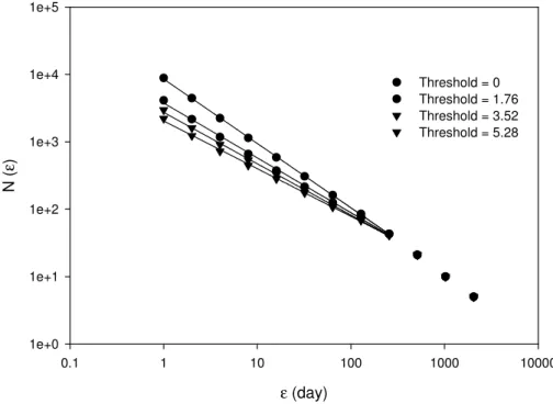
An example of the shifted box-counting graph log N(ε) versus log ε for the runoff time series in sub-watershed W-TB of the Little River watershed is displayed in Fig. 1. The mean daily runoff rate in this example was 3.52 m3s−1(Table 1). Since log N(ε) versus log ε was plotted instead of log N(ε) versus log (1/ε), the value of the negative slope

15

represents the estimated fractal dimension of the sets. The box sizes (time scales) were between one day and 1/5 of the length of the records. If the runoff time series possessed a scale-invariance property, a straight line could be fitted to the box-counting graph or part of it, according to the Eq. (2). Figure 1 shows that for each threshold, two distinct scaling ranges are apparent, each of which can be fitted with a straight-line

20

section by least square regression, instead of a single linear relationship over the entire range of time scales.

The negative slope of each regression line represents the fractal dimension within that scaling range. The existence of linear relationship over certain time scales indi-cates that there is a scale invariant distribution of runoff in time, which is valid within

HESSD

Full Screen / Esc

Print Version Interactive Discussion

EGU

the defined linear scaling range. In fluid mechanics, dimensionless similarity parame-ters such as Reynolds number are used to bridge across scales in hydraulic design. However, it was not feasible to extend this principle of similarity using dimensional pa-rameters to watershed hydrological processes across different scales (Dooge, 1986). By using fractal concepts, temporal scale invariance of runoff might be characterized

5

by a single parameter, fractal dimension (D). Since two D values were obtained from the box-counting analysis for the time series in this example over the time period under consideration, it implies that its scaling properties vary with the time scales.

Likewise, the runoff time series of other five sub-watersheds in the Little River wa-tershed as well as all the sub-wawa-tersheds in the other wawa-tersheds studied (Little Mill

10

Creek watershed, Reynolds Creek watershed, and Sleepers River watershed) all dis-played two scaling ranges for each threshold in their box-counting graphs. The break point (intersection of the two straight line sections in the log N(ε) versus log ε plots) for all thresholds corresponded to the same box size, which indicates the same scaling ranges are valid no matter what runoff intensity threshold was used to define the set.

15

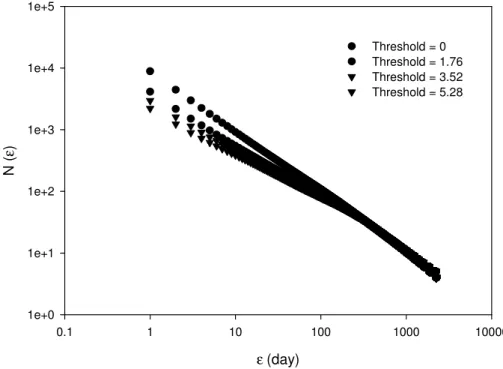
To further precisely locate the break point, the box-counting technique was applied with one-day increment of box size (Fig. 2) instead of the exponential doubling incre-ments used for Fig. 1. In Fig. 2, the break point was found to correspond to a box size of approximately 365 days. This may be explained by the obvious annual cycle of all the runoff time series. The fact that two scaling ranges were apparent would

indi-20

cate that the scaling characteristics of the short-term process (<1 year) and long-term process (>1 year) for watershed runoff were different. Breakpoints in scaling ranges for watershed runoff were also found in other studies using the shifted box-counting analysis. In their investigation of daily flows of the river Warta in Poland, Radziejewski and Kundzewicz (1997) reported a distinct break point in the scaling ranges at

ap-25

proximately 2–4 years. They also detected another less distinct break point located at 10–15 days.

The pattern of multiple scaling segments in box-counting plot has been also ob-served in rainfall time series (Olsson et al., 1992, 1993). The box sizes corresponding

HESSD

Full Screen / Esc

Print Version Interactive Discussion

EGU

to the break points on the plot were related to the average duration of rainfall events and the average duration of dry periods between rainfall events (Olsson et al., 1992). In another study of rainfall, Peters and Christensen (2002) detected a break point of scaling near 3–4 days. They concluded that parameters estimated from the rainfall se-ries could not be used to characterize the frontal system if the estimates are based on

5

observations that are temporally separated by significantly more than 3 days. Multiple scaling ranges seem to be a common phenomenon of natural hydrological series.

Estimated fractal dimensions of the runoff time series are summarized in Table 2 through 5 for each of the four watersheds. If we term the scaling range of box size less than 1 year as range 1, and as 2 otherwise, the fractal dimension in range 1

de-10

creases as the threshold increases. In range 1, for example, D decreases from 0.96 at 0 m3s−1to 0.71 at 5.28 m3s−1for the runoff time series of sub-watershed W-TB (Ta-ble 2). However, the fractal dimensions at range 2 show almost no change for various thresholds with D=1.0 (Fig. 1). The dependence of the estimated fractal dimension on the defined threshold value was also observed in previous studies (Olsson et al., 1992,

15

1993; Radziejewski and Kundzewicz, 1997). In all of these studies, a fractal dimension of 1.0 was obtained when the time scale exceeded a certain value, which was about 365 days in this study.

Naturally, a runoff series of observations has an intermittent pattern. Especially in a dry area, runoff occurs over relatively short durations separated by much longer time

20

intervals of various lengths with no measurable runoff. Therefore, the runoff can be best modeled as a random Cantor set (or Cantor dust), which is a strictly self-similar fractal geometrical object. It is constructed by iteratively removing portions from a line segment of unit length. The size of the portions and their location on the line segment on as well as on the remaining sub-segments are randomly selected. The

25

simplest form of a Cantor set (a non-random set) is created by iteratively removing the central one-third portion of a unit line segment. As the process is repeated to infinity, the sub-segments become shorter and shorter, and form a set of points with various intervals (gaps) between them. If only the days when daily runoff intensity exceeds a

HESSD

Full Screen / Esc

Print Version Interactive Discussion

EGU

selected threshold value are marked, and other days are considered as gaps, then the time structure of a runoff time series would closely resemble a Cantor dust, and their degree of clustering of runoff events can be estimated using the using a random Cantor dust model.

For the runoff series in this study, for the 0 m3s−1threshold, D appropriates or equals

5

to 1.0 for all the runoff series (Tables 2 to 5). This might be because the observations of daily runoff intensity are nearly all greater than 0, therefore, the generated set is almost continuous with few gaps (no runoff) between them. As the threshold increases, the records that are not greater than the threshold are filtered out, and hence more gaps would appear in the newly defined set, and the corresponding Cantor set is sparser.

10

As a result, a smaller dimension was obtained from the box-counting plot. In scaling range 2 where the box sizes are greater than one year the fractal dimension is equal to 1.0 at all the threshold levels (Fig. 1). This might be because there would always have at least one day of a year that the runoff rate exceeded the threshold value. The regression coefficients of regression lines in the log N(ε) versus log ε plots were high

15

for all the runoff time series with values greater than or close to 0.990, which indicates a strong linear relation. These consistently high values are considered requisite to pro-vide confidence in any inference that the runoff series under investigation demonstrate scale invariant characteristics.

Table 2 indicates that the fractal dimensions for all the 6 sub-watersheds of the Little

20

River watershed at each level of the threshold were almost the same, although the contribution areas of these sub-watersheds are quite different (2.6 ∼333.8 km2for sub-watersheds of the Little River watershed as listed in Table 1). For the sub-sub-watersheds of the Little River watershed, the D-value ranged from 0.92 to 0.96 for threshold level 1, 0.81 to 0.83 for level 2, 0.74 to 0.79 for level 3, and 0.68 to 0.71 for level 4 (Table 2).

25

The same pattern was found in all the other three watersheds (Tables 3 through 5). The fractal dimension reflects the degree of irregularity by which the occurrence of an event, such as rainfall, is distributed within a time series (Olsson et al., 1992). Therefore, the estimated dimension of runoff time series might be interpreted as the

HESSD

Full Screen / Esc

Print Version Interactive Discussion

EGU

reflection of the degree of irregularity by which the occurrence of runoff (based on the threshold defined) is distributed. The almost identical fractal dimension of different sub-watersheds at a given threshold level suggests that the irregularity of the runoff distribution in these sub-watersheds has the same pattern, and that the generation of the runoff might follow the same process for those sub-watersheds within a watershed.

5

The results presented in Tables 2 through 5, and the log N(ε) versus log ε box-counting plots for the runoff time series were quite consistent across the sub-watersheds of the four sub-watersheds. With the exception of the two smallest sub-watersheds (W-14 and W-23 of the Reynolds Creek watershed), the same fractal di-mension (estimated using the shifted box-counting method) was obtained for the runoff

10

series at each threshold level although these watersheds varied markedly in climate, topography, and size (Table 1). For example, for a given threshold level, say level 2, the fractal dimension is about 0.85 for practically all the runoff time series in four wa-tersheds (Tables 2 to 5). In other words, runoff time series in these watersheds and their sub-watersheds have similar distribution of occurrence of runoff, and exhibit the

15

same pattern of scaling, although they have different climates, geography, soil type, land management, etc.

It should be pointed out that the threshold values used to define the sets were different for each runoff time series because the mean daily runoff rates of the sub-watersheds were different (Table 1). Selecting threshold values based on mean daily

20

runoff rates allows comparison of the fractal dimensions estimated from different runoff time series. The results indicated that although the daily runoff rates were different by orders of magnitude (Table 1), the occurrence of runoff had the same distribution.

At threshold level 4, the fractal dimensions of runoff time series for the Little Mill Creek and Sleepers River watersheds were slightly less than that for the Little River and

25

Reynolds Creek watersheds. A lower dimension means that more points are clustered in groups over time scales. Thus it indicated that high runoff occurrences are more clustered in the Little Mill Creek and Sleepers River watersheds than the other two watersheds.

HESSD

Full Screen / Esc

Print Version Interactive Discussion

EGU

As discussed above, the occurrence of runoff in agricultural sub-watersheds of vari-ous sizes had similar distribution, making it possible to extrapolate runoff behavior over a fairly large range of spatial scales within a watershed. However, this scaling property may not be valid when the sub-watersheds are small. The box dimension of the runoff series for the two smallest sub-watersheds (W-14=0.01 km2and W-23=0.1 km2) of the

5

Reynolds Creek watershed, were much lower and did not change at different threshold levels (Table 4). It indicated that the distribution of runoff occurrence in extremely small sub-watersheds might be different from larger watersheds, and extrapolation might not be feasible at relatively small scales. One possible explanation might be that the to-tal volume of surface runoff from a very small sub-watershed is limited, and measured

10

runoff tends to be almost zero most of the time depending on the sensitivity and resolu-tion of the measuring instruments. On the other hand, for the runoff series investigated in this study, no upper restriction of sub-watershed size in scaling was detected.

3.2. Estimated Hurst exponent

The Hurst exponent (H) as a useful parameter to describe long-term persistence of

15

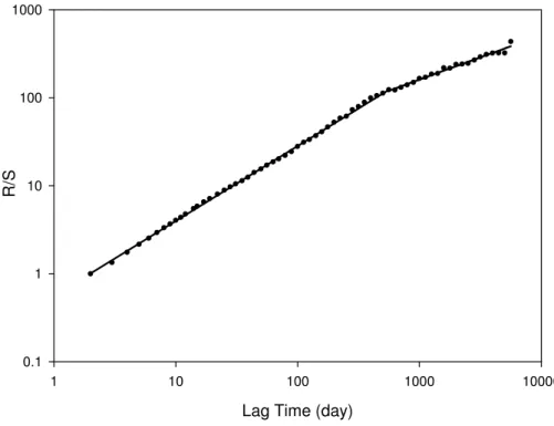
observations in hydrological time series was initially applied in an empirical manner to water reservoir design (Hurst, 1951). It was later established that the Hurst exponent could be theoretically related to the fractal dimension for idealized time series that can be modeled as fractional Brownian motions. Figure 3 shows an example of the rescaled range plot used to obtain the Hurst exponent of the runoff time series for sub-watershed

20

W-TB in the Little River watershed. In the plot, two distinct scaling ranges (denoted as range 1 and range 2) are clearly displayed with a break point at a lag time of about 18 month. A straight line was fitted to each scaling range by least square regression. The regression coefficient of determination (r2) was used to evaluate the goodness of the linear fit. The high value of r2for range 1 (>0.990) indicated a valid scaling range.

25

The rescaled range plots of all runoff time series had two obvious scaling ranges as shown in the example of Fig. 3. The lag time corresponding to the break point of the two scaling ranges was about 15∼18 months, which is consistently greater than the

HESSD

Full Screen / Esc

Print Version Interactive Discussion

EGU

value of about 1 year obtained from box-counting plots (Fig. 1).

The H values of each runoff time series are presented in Table 6. In general, the H values in scaling range 1 (lag time less than the break point) is greater than 0.5 with typical value being above 0.8 (Table 6). An H value greater than 0.5 indicates a persistent process or positive long-term dependence (Mandelbrot and Wallis, 1969).

5

It implies that a greater than average runoff is more likely followed by another greater than average runoff rather than by chance. In other words, the occurrences of the runoff have the tendency to appear in clusters, and the tendency is rather strong as indicated by the high values of H.

Similar H values were obtained for almost all of the runoff time series of

sub-10

watersheds within each watershed (Table 6), which implies that these runoff time se-ries might have similar long-term memory, though their contribution areas are much different. The two smallest sub-watersheds, namely W-14 and W-23 in the Reynolds Creek watershed, had a much smaller H value than the other relatively bigger sub-watersheds. The H value for W-14 is 0.73 and 0.60 for W-23, but about 0.90 for other

15

sub-watersheds in the Reynolds Creek watershed (Table 6). Because the Hurst ex-ponent captures the long-term persistence in the data series, similar values might be interpreted as a reflection of similarities in stable sub-watershed characteristics such as topography, meteorology, and soil type. However, this interpretation may not be applicable at very small scales.

20

The sub-watersheds of the Reynolds Creek and Sleepers River watershed had higher H values than those of the Little River and Little Mill Creek watersheds (Ta-ble 6), although H values were high for all four agricultural watersheds. The H values for the Reynolds Creek and Sleepers River sub-watersheds were about 0.9, and the H values of the other two sub-watershed groupings were about 0.8. As discussed above,

25

the Hurst exponent reflects the long-term dependence of the time series. A higher H value indicates that the previous runoff record will positively affect the future runoff in-tensity, thus an extreme event would have higher probability of being followed by other extreme events.

HESSD

Full Screen / Esc

Print Version Interactive Discussion

EGU

In comparison with scaling range 1, the H-values for scaling range 2 above the break point were smaller and more variable among the sub-watersheds than for range 1. Also, the linear fits had smaller r2values, indicating that the scaling property in range 2 was not as persistent as in range 1. The smaller H values in range 2 imply that the strong long-term persistence dissipates beyond the lag time of about 15∼18 months.

5

In other words, observations in the runoff record separated by 15 months or more have little or no impact on each other. For the Little River and Little Mill Creek sub-watershed groups, H values ranged from 0.46 to 0.53 (Table 6) for scaling range 2, indicating a random process (Mandelbrot and Wallis, 1969). This implies that the impact of past events on future runoff basically disappeared after 15∼18 months. For the Sleepers

10

River sub-watershed group, the H values were even smaller, much less than 0.50 (Ta-ble 6) indicating anti-persistence.

As previously indicated, the W-14 and W-23 sub-watersheds of the Reynolds Creek watershed have much different fractal dimension and Hurst exponent in comparison with other sub-watersheds, which might be explained by their relatively small size

15

(0.1 km2 and 0.01 km2). Watershed hydrological response (e.g. surface runoff), is a function of the size of the area being considered. The effect of underlying hetero-geneity on such response is somewhat random at smaller scales, but becomes more systematic at larger scales (DeCoursey, 1996). General terms such as local scale, hill-slope scale, and catchment scale are often used to distinguish different spatial scales

20

in hydrology (Kirkby, 1988). It is generally recognized that the dominance of various watershed features changes as scale changes. For example, soil properties dominate at local and hillslope scale, while the topography and basin morphology are impor-tant at the larger scale. However, the watershed size ranges that validly define these scales are hard to determine, since it would depend on the topography, soils, climate

25

and other factors of the watershed. For example, it could be a square kilometer or larger in dry climates with gentle slope and sandy soils, but a hectare or less in humid areas with loam soils (DeCoursey, 1996). The analyses by Wood et al. (1988) showed plotted runoff and infiltration volume against catchment area showed a convergence of

HESSD

Full Screen / Esc

Print Version Interactive Discussion

EGU

mean runoff and infiltration volumes at about 1.0 km2. This area was described as a Representative Elementary Area (REA), which is a function of the particular catchment and climatic characterization and general topography. The REA’s of two catchments (4.4 and 631 ha) were found to be 0.02–0.03 and 2.5–3.5 km2 for the small and large areas, respectively (Goodrich et al., 1993). When the catchments are greater than the

5

REA, the hydrological response of individual catchments becomes alike even though the patterns of properties within each catchment may be different (DeCoursey, 1996).

4. Conclusions

The scaling property of daily runoff for 32 sub-watersheds covering a wide range of sizes in four agricultural watersheds of different climate and topography was examined

10

using the shifted box-counting method and Hurst rescaled range analysis. The results showed that long-term records of daily runoff rate exhibited scale invariance over cer-tain time scales. Two scaling ranges were identified in the shifted box-counting plots with a break point at about 12 months. The Hurst analysis showed that the runoff time series also displayed a rather strong long-term persistence which dissipated

af-15

ter 15∼18 months. The same fractal dimensions and Hurst exponents were obtained for the sub-watersheds within each watershed, indicating that the runoff of these sub-watersheds have similar distribution of occurrence and similar long-term memory.

These results indicated the existence of scale invariance in the runoff time series in agricultural watersheds over temporal and spatial scales. This finding would imply

20

the theoretical possibility of deriving short-term estimates from longer-term measure-ments or vice versa, or to transfer information about runoff data and runoff processes from gauged to ungauged areas. Extrapolation between scales of observations and between watersheds would reduce the extent and degree of monitoring data required by legislative mandates or model simulation and lead to significant savings in cost and

25

HESSD

Full Screen / Esc

Print Version Interactive Discussion

EGU

References

Bloschl, G. and Sivapalan, M.: Scale issues in hydrological modeling: a review, Chapter 2, in: Scale Issues In Hydrological Modelling, John Wiley & Sons, New York, 1995.

DeCoursey, D. G.: Hydrological, climatological, and ecological systems scaling: A review of selected literature and comments, Interim Progress Report, USDA-ARS-NPA, GRSRU, Fort

5

Collins, CO 80522, 1996.

Dooge, J. C. I.: Looking for hydrologic laws, Water Resour. Res., 22, 46–58, 1986.

Goodrich, D. C., Woolhiser, D. A., and Sorooshian, S.: A stabilization measure for stream net-work complexity and application of REA concepts to semi-arid watersheds, in: Scale Issues in Hydrological/Enviormental Modeling, edited by: Kalma, J., Sivapalan, M., and Wood, E.,

10

CSIRO-UAW-ANU, 1993.

Gupta, V. K. and Waymire, E.: On Taylor’s hypothesis and dissipation in rainfall, J. Geophys. Res., 92, 9657–9660, 1987.

Gupta, V. K. and Waymire, E.: A statistical analysis of mesoscale rainfall as a random cascade, J. App. Meteo., 32, 251–267, 1993.

15

Gupta, V. K., Castro, S. L., and Over, T. M.: On scaling exponents of spatial peak flows from rainfall and river network geometry, J. Hydrol., 187, 81–104, 1996.

Hurst, H. E.: The long term storage capacity of reservoirs, Tran. ASCE, 116, 770–808, 1951. Kirkby, M. J.: Hillslope runoff processes and models, J. Hydrol., 100, 315–339, 1988.

Labat, D., Mangin A., and Ababou, R.: Rainfall-runoff relations for karstic springs: multifractal

20

analysis, J. Hydrol., 256, 176–195, 2002.

Lovejoy, S. and Schertzer, D.: Generalized scale invariance and fractal models of rain, Water Resour. Res., 21, 1233–1250, 1985.

Mandelbrot, B. B. and Wallis, J. R.: Some long-run properties of geophysical records, Water Resour. Res., 5, 321–340, 1969.

25

Mandelbrot, B. B.: The fractal geometry of nature, W. H. Freeman, New York, 1983.

Menabde, M., Harris, D., Seed, A., Austin, G., and Stow, D.: Multiscaling properties of rainfall and bounded random cascade, Water Resour. Res., 33, 2823–2830, 1997.

National Research Council, US: Committee on Opportunities in the Hydrologic Science, Na-tional Academy Press, Washington, 1991.

30

Olsson, J., Niemczynowicz, J., Berndtsson, R., and Larson, M.: An analysis of the rainfall time structure by box-counting-some practical implications, J. Hydrol., 137, 261–277, 1992.

HESSD

Full Screen / Esc

Print Version Interactive Discussion

EGU

Olsson, J., Niemczynowicz, J., and Berndtsson R.: Fractal analysis of high-resolution rainfall time series, J. Geophys. Res., 98, 23 265–23 274, 1993.

Pandey, G., Lovejoy, S., and Schertzer, D.: Multifractal analysis of daily river flows including extremes for basins of five to two million square kilometers, one day to 75 years, J. Hydrol., 208, 62–81, 1998.

5

Peters, E. E.: Fractal market analysis: applying chaos theory to investment, John Wiley & Sons Inc., New York, 1994.

Peters, O. and Christensen, K.: Rain: relaxation in the sky, Phys. Rev. E., 66, 1–9, 2002. Radziejewski, M. and Kundzewicz, Z. W.: Fractal analysis of flow of the river Warta, J. Hydrol.,

200, 280–294, 1997.

10

Robinson, J. S. and Sivapalan, M.: Temporal scales and hydrological regimes: Implications for flood frequency scaling, Water Resour. Res., 33, 2981–2999, 1997.

Rodriguez-Iturbe, I. and Rinaldo, A.: Fractal river basins: chance and self-organization, Cam-bridge Univ. Press, New York, 1997.

Schertzer, D. and Lovejoy, S.: Physical modeling and analysis of rain and clouds by anisotropic

15

scaling multiplicative processes, J. Geophys. Res., 92, 9693–9714, 1987.

Schmitt, F., Vannitsem, S., and Barbosa, A.: Modeling of rainfall time series using two-state renewal processes and multifractals, J. Geophys. Res., 103, 23 181–23 193, 1998.

Sposito, G.: Scale dependence and scale invariance in hydrology, Cambridge, United Kingdom, 1998.

20

USEPA: The quality of our nation’s water, Report 841-S-94-002, US Environmental Protection Agency, Washington, D.C., 1995.

Wood, E. F., Sivapalan, M., Beven, K., and Band, L.: Effects of spatial variability and scale with implications to hydrological modeling, J. Hydrol., 102, 29–47, 1988.

HESSD

Full Screen / Esc

Print Version Interactive Discussion

EGU Table 1. Properties of agricultural watersheds and sub-watersheds studied.

Watershed Sub-watershed Area Record period Daily mean runoff rate

(km2) (m3s−1)

W-TB 333.8 11/01/1971–30/09/2002 3.52 W-TF 114.8 01/01/1969–30/09/2002 1.33 Little River W-TI 49.9 01/01/1969–30/09/2002 0.67 watershed W-TJ 22.1 01/01/1969–30/09/2002 0.29 W-TK 16.7 01/01/1969–30/09/2002 0.21 W-TM 2.6 01/01/1969–31/12/1988 0.03 W-5 1.4 01/10/1938–01/10/1971 0.012 W-10 0.5 05/10/1938–01/10/1971 0.004 W-91 0.32 01/10/1938–01/10/1971 0.011 Little Mill W-92 3.7 01/10/1938–01/10/1971 0.035 Creek watershed W-94 6.2 01/10/1938–01/10/1971 0.059 W-95 11.1 01/10/1938–22/06/1972 0.098 W-97 18.5 01/01/1937–01/10/1971 0.181 W-1 233.5 01/01/1963–30/09/1996 0.56 W-2 36.4 29/01/1964–15/04/1994 0.082 W-3 31.8 13/03/1964–31/12/1990 0.072 W-4 54.4 29/03/1966–30/09/1996 0.42 Reynolds Creek W-11 1.2 01/01/1967–31/12/1977 0.0075 watershed W-13 0.4 01/01/1963–30/09/1996 0.0067 W-14 0.1 07/031996–17/04/1984 0.000041 W-15 0.5 01/10/1964–31/12/1984 0.0069 W-16 14.1 01/01/1973–20/12/1980 0.13 W-23 0.01 15/01/1972–30/09/1996 0.00000057 W-1 42.9 23/01/1959–30/12/1973 0.67 W-2 0.6 01/01/1961–29/11/1971 0.0073 W-3 8.4 01/01/1960–01/02/1979 0.16 Sleepers River W-4 43.5 01/01/1960–30/12/1973 0.72 watershed W-5 111.2 01/01/1960–30/12/1973 1.97 W-7 21.8 01/01/1961–30/12/1972 0.34 W-8 15.6 01/01/1961–15/05/1979 0.24 W-9 0.5 15/09/1961–10/07/1973 0.0076 W-11 2.3 01/05/1964–23/11/1972 0.026

HESSD

Full Screen / Esc

Print Version Interactive Discussion

EGU Table 2. Fractal dimensions of daily runoff rate for six sub-watersheds of the Little River

wa-tershed in Tifton, Georgia. Fractal dimensions corresponding to four threshold levels of the runoff rate (0, 0.5M, M, and 1.5M, where M is the daily mean runoff rate) were obtained as the absolute value of the slope of straight lines fitted to plots as shown in Fig. 1.

Sub-watershed Threshold (m3s−1) Fractal dimension (D) r2

0 0.96 0.999 W-TB 1.76 0.81 0.998 3.52 0.76 0.997 5.28 0.71 0.994 0 0.94 0.999 W-TF 0.66 0.83 0.998 1.33 0.77 0.995 2.00 0.71 0.991 0 0.93 0.999 W-TI 0.33 0.83 0.997 0.67 0.77 0.995 1.00 0.70 0.991 0 0.92 0.999 W-TJ 0.15 0.81 0.996 0.30 0.74 0.994 0.45 0.68 0.990 0 0.92 0.999 W-TK 0.10 0.84 0.997 0.20 0.79 0.996 0.30 0.73 0.994 0 0.96 0.999 W-TM 0.015 0.83 0.998 0.030 0.76 0.996 0.045 0.69 0.991

HESSD

Full Screen / Esc

Print Version Interactive Discussion

EGU Table 3. Fractal dimensions of daily runoff rate for seven sub-watersheds of the Little Mill Creek

watershed in Coshocton, Ohio. Fractal dimensions corresponding to four threshold levels of the runoff rate (0, 0.5M, M, and 1.5M, where M is the daily mean runoff rate) were obtained as the absolute value of the slope of straight lines fitted to plots as shown in Fig. 1.

Sub-watershed Threshold (m3s−1) Fractal dimension (D) r2

0 1.00 0.999 W-5 0.006 0.83 0.995 0.012 0.75 0.991 0.018 0.69 0.986 0 0.99 0.999 W-10 0.002 0.79 0.995 0.004 0.71 0.990 0.006 0.63 0.983 0 1.01 0.999 W-91 0.0057 0.82 0.996 0.011 0.75 0.991 0.172 0.67 0.985 0 0.99 0.999 W-92 0.018 0.82 0.999 0.036 0.74 0.999 0.054 0.66 0.998 0 1.00 0.999 W-94 0.03 0.82 0.996 0.06 0.73 0.991 0.09 0.66 0.985 0 0.99 0.999 W-95 0.049 0.82 0.997 0.098 0.73 0.993 0.147 0.67 0.989 0 1.00 0.999 W-97 0.09 0.82 0.997 0.18 0.73 0.993 0.27 0.64 0.987

HESSD

Full Screen / Esc

Print Version Interactive Discussion

EGU Table 4. Fractal dimensions of daily runoff rate for ten sub-watersheds of the Reynolds Creek

watershed in Boise, Idaho. Fractal dimensions corresponding to four threshold levels of the runoff rate (0, 0.5M, M, and 1.5M, where M is the daily mean runoff rate) were obtained as the absolute value of the slope of straight lines fitted to plots as shown in Fig. 1.

Sub-watershed Threshold (m3s−1) Fractal dimension (D) r2

0 1.00 0.999 W-1 0.28 0.82 0.997 0.56 0.77 0.996 0.84 0.72 0.994 0 1.00 0.999 W-2 0.041 0.85 0.998 0.082 0.76 0.996 0.123 0.70 0.994 0 1.00 0.999 W-3 0.036 0.81 0.998 0.072 0.74 0.996 0.108 0.68 0.995 0 1.00 0.999 W-4 0.21 0.82 0.997 0.42 0.75 0.996 0.63 0.72 0.994 hline 0 0.98 0.999 W-11 0.0038 0.84 0.998 0.0075 0.77 0.998 0.0113 0.72 0.997 0 1.00 0.999 W-13 0.0034 0.76 0.993 0.0067 0.80 0.990 0.0100 0.79 0.989 0 0.72 0.994 W-14 0.00002 0.67 0.995 0.00004 0.65 0.995 0.00006 0.63 0.993

HESSD

Full Screen / Esc

Print Version Interactive Discussion

EGU Table 4. Continued.

Sub-watershed Threshold (m3s−1) Fractal dimension (D) r2

0 0.99 0.999 W-15 0.0035 0.77 0.995 0.0070 0.73 0.992 0.0105 0.70 0.991 0 1.00 0.999 W-16 0.065 0.84 0.999 0.130 0.77 0.998 0.195 0.74 0.996 W-23 0 0.41 0.976 0.00000028 0.41 0.976 0.00000057 0.41 0.976 0.00000084 0.41 0.977

HESSD

Full Screen / Esc

Print Version Interactive Discussion

EGU Table 5. Fractal dimensions of daily runoff rate for nine sub-watersheds of the Sleepers Creek

watershed in Vermont. Fractal dimensions corresponding to four threshold levels of the runoff rate (0, 0.5M, M, and 1.5M, where M is the daily mean runoff rate) were obtained as the absolute value of the slope of straight lines fitted to plots as shown in Fig. 1.

Sub-watershed Threshold (m3s−1) Fractal dimension (D) r2

0 1.00 0.999 W-1 0.34 0.86 0.997 0.67 0.73 0.991 1.00 0.67 0.987 0 1.00 0.999 W-2 0.0036 0.88 0.997 0.0072 0.76 0.995 0.0108 0.65 0.986 0 1.00 0.999 W-3 0.08 0.88 0.998 0.16 0.74 0.992 0.24 0.65 0.987 0 1.00 0.999 W-4 0.36 0.87 0.997 0.72 0.74 0.992 1.08 0.67 0.991 0 1.00 0.999 W-5 0.98 0.87 0.997 1.97 0.75 0.992 2.95 0.67 0.989 0 1.00 0.999 W-7 0.17 0.86 0.997 0.34 0.73 0.994 0.51 0.67 0.989 0 1.00 0.999 W-8 0.12 0.84 0.999 0.24 0.73 0.994 0.36 0.66 0.989

HESSD

Full Screen / Esc

Print Version Interactive Discussion

EGU Table 5. Continued.

Sub-watershed Threshold (m3s−1) Fractal dimension (D) r2

0 0.98 0.999 W-9 0.0038 0.83 0.998 0.0076 0.73 0.995 0.0114 0.66 0.994 0 0.99 0.999 W-11 0.013 0.85 0.999 0.026 0.77 0.995 0.039 0.69 0.992

HESSD

Full Screen / Esc

Print Version Interactive Discussion

EGU Table 6. Hurst exponent (H) of daily runoff time series estimated using the R/S analysis

method. Scaling range 1 corresponds to the lag time less than the break point of rescaled range plot, and range 2 corresponds to the lag time greater than the break point. H for each range was obtained as the slope of fitted straight lines to plots as shown in Fig. 3.

Watershed Sub-watershed Range 1 Range 2

H r2 H r2

W-TB 0.85 0.999 0.50 0.992

W-TF 0.85 0.998 0.49 0.983

Little River W-TI 0.82 0.999 0.48 0.988

watershed W-TJ 0.82 0.998 0.51 0.989 W-TK 0.83 0.997 0.51 0.986 W-TM 0.81 0.997 0.46 0.981 Average 0.83 0.49 W-5 0.83 0.999 0.52 0.988 W-10 0.80 0.999 0.51 0.989 W-91 0.85 0.999 0.46 0.991

Little Mill Creek W-92 0.83 0.999 0.46 0.993

watershed W-94 0.82 0.999 0.47 0.992 W-95 0.83 0.999 0.46 0.991 W-97 0.80 0.999 0.53 0.990 Average 0.82 0.49 W-1 0.92 0.999 0.60 0.973 W-2 0.92 0.999 0.54 0.983 W-3 0.89 0.999 0.60 0.991 W-4 0.95 0.999 0.59 0.978 Reynolds Creek W-11 0.92 0.999 0.53 0.972 watershed W-13 0.93 0.999 0.43 0.971 W-14 0.73 0.999 0.60 0.985 W-15 0.92 0.999 0.35 0.988 W-16 0.96 0.999 0.27 0.970 W-23 0.60 0.996 0.37 0.984 Average 0.87 0.49

HESSD

Full Screen / Esc

Print Version Interactive Discussion

EGU Table 6. Continued.

Watershed Sub-watershed Range 1 Range 2

H r2 H r2 W-1 0.88 0.998 0.45 0.795 W-2 0.87 0.998 0.30 0.892 W-3 0.90 0.998 0.41 0.952 Sleepers River W-4 0.91 0.997 0.32 0.888 watershed W-5 0.90 0.997 0.29 0.810 W-7 0.87 0.998 0.39 0.958 W-8 0.91 0.998 0.35 0.947 W-9 0.91 0.999 0.42 0.709 W-11 0.92 0.997 0.63 0.758 Average 0.90 0.40

HESSD

Full Screen / Esc

Print Version Interactive Discussion EGU ε ε (day) 0.1 1 10 100 1000 10000 N ( ε) 1e+0 1e+1 1e+2 1e+3 1e+4 1e+5 Threshold = 0 Threshold = 1.76 Threshold = 3.52 Threshold = 5.28 Figure 1

Fig. 1. Log-log plots of number of boxes (N(ε)) versus box size (ε) for different threshold values

(0, 1.76, 3.52, and 5.28 m3/s) using the shifted box counting method to analyze the runoff rate series for sub-watershed W-TB of the Litter River watershed in Tifton, Georgia. In all cases, r2 was >0.990 for the straight lines fitted to the sections of the graph. Box sizes were exponentially doubled starting at ε=1 day.

HESSD

Full Screen / Esc

Print Version Interactive Discussion EGU ε (day) 0.1 1 10 100 1000 10000 N ( ε) 1e+0 1e+1 1e+2 1e+3 1e+4 1e+5 Threshold = 0 Threshold = 1.76 Threshold = 3.52 Threshold = 5.28

Figure 2. Shifted box counting graph as in Figure 1 but with oneFigure 2

Fig. 2. Shifted box counting graph as in Fig. 1 but with one day increment of box size (ε) for

sub-watershed W-TB of the Litter River watershed in Tifton, Georgia. The break point of the slope occurs at approximately ε=365 days.

HESSD

Full Screen / Esc

Print Version Interactive Discussion

EGU

Lag Time (day)

1 10 100 1000 10000 R /S 0.1 1 10 100 1000 Figure 3

Fig. 3. Hurst rescaled range analysis plot for sub-watershed W-TB of the Little River watershed

in Tifton, Georgia. A scaling break point occurs at about 18 months. r2 was >0.99 for the straight lines fitted to each scaling range.