Continuous observation planning for autonomous exploration

(1)

Continuous Observation Planning for Autonomous Exploration

by

Bradley R. Hasegawa

Submitted to the Department of Electrical Engineering and Computer Science in Partial Fulfillment of the Requirements for the Degree of

Master of Engineering in Electrical Engineering and Computer Science

at the Massachusetts Institute of Technology

MASSACHUSETTS INSTfTUE

August 17, 2004 %-Lv 2Oe -i OF TECHNOLOGY

JUL

18 2005

LIBRARIES

The author hereby grants to M.I.T. permission to reproduce and

distribute publicly paper and electronic copies of this thesis and to grant others the right to do so.

Author

Department of Electrical Engine tr 'ence

Augupt l/, 2004 Certified by_ /John J. Leonard Thesis Supervisor Bria C. Williams Tsor Certified by Accepted by Arthur C. Smith

(2)

(3)

Continuous Observation Planning for Autonomous Exploration

by

Bradley R. Hasegawa

Submitted to the

Department of Electrical Engineering and Computer Science

August 17, 2004

In Partial Fulfillment of the Requirements for the Degree of Master of Engineering in Electrical Engineering and Computer Science

ABSTRACT

Many applications of autonomous robots depend on the robot being able to navigate in real world environments. In order to navigate or path plan, the robot often needs to consult a map of its surroundings. A truly autonomous robot must, therefore, be able to drive about its environment and use its sensors to build a map before performing any tasks that require this map. Algorithms that control a robot's motion for the purpose of building a map of an environment are called autonomous exploration algorithms.

Because resources such as time and energy are highly constrained in many mobile robot missions, a key requirement of autonomous exploration algorithms is that they cause the robot to explore efficiently. Planning paths to candidate observation points that will lead to efficient exploration is challenging, however, because the set of candidates, and, therefore, the robot's plan, change frequently as the robot adds information to the map. The main claim of this thesis is that, in situations in which the robot discerns the large scale structure of the environment early on during its exploration, the robot can produce paths that cause it to explore efficiently by planning observations to make over a finite horizon. Planning over a finite horizon entails finding a path that visits candidates with the maximum possible total utility, subject to the constraint that the path cost is less than a given threshold value. Finding such a path corresponds to solving the Selective

Traveling Salesman Problem (S-TSP) over the set of candidates. In this thesis, we

evaluate our claim by implementing full horizon, finite horizon, and greedy approaches to planning observations, and comparing the efficiency of these approaches in both real and

simulated environments. In addition, we develop a new approach for solving the S-TSP

by framing it as an Optimal Constraint Satisfaction Problem (OCSP).

Thesis Supervisor: John J. Leonard

Title: Associate Professor of Ocean Engineering Thesis Supervisor: Brian C. Williams

(4)

(5)

List of Figures

Figure 1.1 Exam ple of a Line Feature M ap ... 13

Figure 1.2 Candidate Identification and Scoring with Newman, Bosse, and Leonard M eth o d ... 15

Figure 1.3 Example of Knowing Large Scale Structure Beforehand ... 21

Figure 1.4 Architecture of Experimental System... 25

Figure 2.1 Pseudo-code for Exploration using Basic Exploration Path Planning ... 33

Figure 2.2 Pseudo-code for Exploration using Continuous Exploration Path Planning ... 34

Figure 2.3 M atching Sensor Scans... 36

Figure 2.4 A Simple Occupancy Grid M ap... 37

Figure 2.5 A Line Feature SLAM M ap... 39

Figure 2.6 Candidate Scoring for the Gonzalez-Banos and Latombe Method ... 46

Figure 2.7 Candidate Observation Points for a Partial Map... 52

Figure 2.8 Evaluating Candidate Observation Points ... 54

Figure 3.1 Possible G reedy Functions ... 65

Figure 3.2 The Inefficiency of Greedy Paths ... 66

Figure 3.3 When the Full Horizon Path Performs Worse than Greedy... 69

Figure 3.4 When a Change in the Set of Candidates Helps the Full Horizon Method ... 70

Figure 3.5 Finite Horizon Paths for L=5 and L=1 I... 73

Figure 3.6 Receding Horizon (a) versus Fixed Horizon (b)... 81

Figure 3.7 Extracting a Graph for the S-TSP... 86

Figure 3.8 Pseudo-code for the Finite Horizon Observation Planning Method...87

Figure 3.9 Pseudo-code for Receding and Fixed Horizon Approaches to Exploration.... 89

Figure 3.10 Getting Interrupted after Making a Sacrifice ... 93

Figure 3.11 Exploration Without Changing the Set of Candidates ... 97

Figure 3.12 Candidate Interactions ... 100

Figure 3.13 Going to Explored Regions over Unexplored Regions ... 101

Figure 4.1 OCSP Formulation of an S-TSP Instance ... 107

Figure 4.2 Pseudo-code for Constraint-based A* ... 109

Figure 4.3 Partial Search Tree for Constraint-based A* ... 112

Figure 4.4 Search Node Expansion Functions ... 113

Figure 4.5 Node Expansion in Constraint-based A*... 115

Figure 4.6 Solving an S-TSP with Constraint-based A*... 117

Figure 4.7 Converting an Undirected Graph into a Directed Graph... 119

Figure 4.8 Converting a Directed Graph into an Undirected Graph... 121

Figure 4.9 Graph Transformations for S-TSP Example... 121

Figure 5.1 Architecture of Experimental System ... 124

Figure 5.2 Pseudo-code for SLAM Process and Exploration Method Process ... 125

Figure 5.3 Candidate Graph Extraction Pseudo-code ... 131

Figure 5.4 Methods of Extracting Obstacles from a Line Map ... 133

Figure 5.5 Maps from the First Moment (a) and Second Moment (b)... 137

Figure 5.6 Candidate Identification and Scoring for the First Moment... 138

Figure 5.7 Obstacles (a) and the Visibility Graph (b) for the First Moment ... 139

Figure 5.8 Extracting the Candidate Graph from D* Instances... 140

(8)

Figure 5.10 Candidate Identification and Scoring for the Second Moment ... 143

Figure 5.11 Visibility Graph for the Second M oment... 143

Figure 5.12 Searching the Visibility Graph Incrementally... 145

Figure 5.13 Candidate Graph for the Second Moment... 146

Figure 5.14 Final Exploration Path for the Second Moment... 147

Figure 6.1 Explored Region for the Final Map of the First Greedy Trial in NE43Floor8 ...152

Figure 6.2 Candidates Disappearing and Appearing Because of Line Movement ... 164

Figure 6.3 Beginning of the Second NE43Floor8 i5m Receding Horizon Trial ... 166

Figure 6.4 Beginning of the Second NE43Floor8 15m Receding Horizon Trial Continued ...168

Figure 6.5 Visiting Explored Regions Over Unexplored Regions ... 170

Figure 6.6 Screenshots of Exploration of BuildingIOFloori with a 15m Fixed Horizon172 Figure 6.7 Final Maps of Short Horizon and Greedy Trials in Building I1Floori and N E 4 3F loor8 ... 174

Figure 6.8 Candidates in a New Room While Exploring NE43Floor8 ... 175

Figure 6.9 Initial Exploration Paths through the StructuredRocks Environment ... 179

Figure 6.10 First Third of BuildingIFloorI 30m Receding Horizon Trial... 180

Figure 6.11 Second Third of Building IFloor 1 30m Receding Horizon Trial ... 181

Figure 6.12 Final Third of Building 1 OFloori 30m Receding Horizon Trial... 183

Figure 6.13 Final Maps for the BuildinglOFloori Greedy and 30m Receding Horizon T ria ls ... 18 4 Figure 6.14 Final Maps for the BuildingIOFloorI 15m and 30m Receding Horizon Trials ...185

Figure 6.15 Final Maps for Real Buildings 34 and 36 Trials ... 188

Figure 6.16 Why the Greedy Trial Got to the Elevator Lobby... 190

Figure 6.17 Middle of the 30m Receding Horizon Trial... 191

Figure 6.18 Final M aps of Trials in 15byi5Room ... 193

Figure 6.19 Part of the 15m Fixed Horizon Trial... 196

Figure 6.20 Moments in the 25by45Room Full Horizon Trial... 198

Figure 6.21 Difficulties Exploring around Squares in RandomRocks 8m Fixed Horizon T ria l ... 2 0 1

(9)

List of Tables

Table 3.1 Least-Cost Paths Between Candidates with Path Cost 11 m... 74

Table 6.1 Performance of Observation Planning Methods in NE43Floor8... 159

Table 6.2 Performance of Observation Planning Methods in Building I OFloorl ... 159

Table 6.3 Performance of Observation Planning Methods in i5byi5Room... 160

Table 6.4 Performance of Observation Planning Methods in 25by45Room... 160

Table 6.5 Performance of Observation Planning Methods in RandomRocks ... 160

Table 6.6 Performance of Observation Planning Methods in Real Buildings 34 and 36161 Table 6.7 Results of Visiting Every Candidate in 15by 15Room... 194

(10)

Acknowledgements

First and foremost, I would like to thank my advisors, Professor Brian Williams and Professor John Leonard for believing in me and for giving me the opportunity to be a part of their groups. I am especially grateful for all of the time and effort both of my advisors have put into helping me and thinking through problems with me. In my mind, Professor Williams and Professor Leonard have gone above and beyond the call of duty in order to advise me, and I have learned more from my interactions with them than from anything else over this past year.

I am also very grateful to Paul Robertson, Seung Chung, Lars Blackmore, Paul

Elliott, John Stedl, Ed Olson, and Jonathan Kennel for their extremely helpful feedback and thoughts on this thesis. In addition, I would like to thank Margaret Yoon, the former administrative assistant to Professor Williams' group, for all of her help in getting this research completed.

I have also received invaluable support and knowledge from I-hsiang Shu,

Andrew Patrikalakis, Stanislav Funiak, Oliver Martin, Matt Walter, Mike Bosse, Sung Joon Kim, Raj Krishnan, Tazeen Mahtab, Martin Sachenbacher, Thomas Leaute, Bobby Effinger, Greg Sullivan, Aisha Walcott, Jillian Redfern, Andreas Hoffman, Steve Block, Tsoline Mikaelian, Judy Chen, Hui Li, Mike Benjamin, and all of the other members of Professor Williams and Professor Leonard's research groups. I feel very fortunate to have had not one but two amazing groups of people to work with.

I could not have made it through the year without my friends and family. In

particular, I would like to thank T. D. Luckett and Michael Ogrydziak for putting up with me when most other people probably would not have.

Finally, I owe very special thanks to my parents for all of their sacrifices, for all of the opportunities that they have given me, for their support and advice, and for always being there for me. I am incredibly lucky to have gotten the parents that I have.

This research was supported by the NASA Ames Cross Enterprise Technology Development Program (CETDP), contract NAG2-14660NR, and by the Office of Naval Research, awards NOOO 14-03-1-0879 and NOGO 14-02-C-0210.

(11)

1 Introduction

There are a vast number of potential applications for autonomous robots that can move about and act on the physical world. Some of the most important uses of these robots are situations in which it is too dangerous, costly, or technologically difficult to send humans to perform a task. These situations are challenging because they require the robot to operate in the noisy and unpredictable real world, as opposed to carefully

controlled factory floors. Recent advances, however, have put robots for many of these applications within reach. Specifically, researchers have worked on rovers for exploring Mars [25], autonomous underwater vehicles (AUVs) for detecting ocean mines [46] and conducting oceanographic surveys [3], unmanned air vehicles (UAVs) for surveillance

[27], and urban robots for performing building search and rescue [11] or assisting the growing elderly population [39].

A fundamental problem for all autonomous mobile robots is being able to

navigate and reason about the surrounding environment. In many cases, the only way for a robot to solve this problem is to consult an internal model (map) of its environment. For example, a very simple navigation task for an AUV could be to travel forward 50 meters, make a 90 degree turn, and then travel straight for 25 more meters. The AUV could try to traverse paths like this one using dead-reckoning, yet eventually it would find itself unacceptably far off course. The problem is that in all methods of dead-reckoning, including inertial guidance systems and odometry for wheeled robots, the navigation error accumulates over time. Furthermore, in space, underwater, and indoors, GPS is not available to help a robot to navigate. Therefore, the robot must use its sensors to

recognize landmarks and localize itself within a map of the environment, in order to bound its navigation error. More sophisticated spatial reasoning, such as planning a path between two points that avoids obstacles, also requires a mobile robot to have a map of the surroundings.

The main problem with a robot relying on maps is that, for many environments, such maps do not exist. Fortunately, researchers have developed algorithms that allow a robot to use its sensors to build a map of its environment and at the same time localize

(12)

itself within this map. In other words, these algorithms allow a robot to perform simultaneous localization and mapping (SLAM) [12] [34] [32]. SLAM algorithms passively process sensor and dead-reckoning data in order to build the best map possible of the part of the environment that the robot has seen. However, these algorithms do not actively move the robot in order to add information to the map. Often, a robot cannot construct an adequate map as it performs its mission; therefore, it must drive about its environment and build a map before it performs actions requiring this map. Algorithms for actively controlling a robot's actions for the purpose of adding information to the robot's map are called autonomous exploration algorithms.

Unfortunately, resources such as time or energy are highly constrained in many autonomous robotics missions [4]. For a robot to spend a lot of time or energy driving around and building a map before it even begins performing its intended mission is

highly undesirable. As a result, a key requirement for methods of autonomous

exploration is that they cause the robot to build the best map possible, while using resources as efficiently as possible. The larger the environment is, the bigger the

potential exists for a robot to waste significant resources mapping that environment, and hence the more important it is for the robot's exploration strategy to be efficient.

Although a number of methods of autonomous exploration have been developed, little work has been done on optimizing the efficiency of these methods. Therefore, this thesis develops and evaluates general methods of planning observations during

exploration in order to improve efficiency. A major contribution of this thesis is the development of a family of methods for planning observations over a finite horizon called finite horizon methods. In order to facilitate evaluation, we implemented and tested a variety of observation planning methods on a real and simulated robot.

In the next section we explain in more detail how SLAM algorithms and

autonomous exploration algorithms work. Then, building on this explanation, we explain what it means to plan observations for autonomous exploration. We then provide a precise problem statement for the thesis, and explain the technical challenges that this problem statement presents. We next outline the architecture of the autonomous

exploration system that we implemented and tested. Finally, we enumerate the claims of this thesis.

(13)

1.1 SLAM and Autonomous Exploration

SLAM algorithms take data from a robot's sensors and dead-reckoning system,

and produce a map of the environment and an estimate of the robot's position within this map. These algorithms usually use state estimation techniques to keep track of the robot's estimate of the position of objects in the environment, as well as its uncertainty in these positions. There are a number of different map representations that SLAM

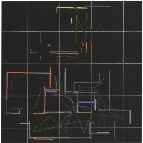
algorithms use, including occupancy grid maps [13], scan-matched maps [18] [49] [21], and feature maps [44]. The autonomous exploration implementation that we test in this thesis uses line feature maps. Line feature-based SLAM only adds objects to its map that can be reasonably represented as a line. Selectively adding objects to the map avoids the computational burden of estimating the position of every point that the robot's sensors have ever seen. Figure 1.1 shows a typical line feature map. The thin line winding through the map is the robot's estimated path through the environment.

(14)

Because SLAM algorithms keep track of both the estimated positions of objects in the environment and the uncertainty in these position estimates, there are two categories

of approaches to autonomous exploration. Exploration algorithms in the first category aim to decrease the map's uncertainty about the positions of objects, by having the robot re-observe these objects. Exploration algorithms in the second category aim to increase the map's coverage by having the robot observe areas it has never seen before. Less work has been done on improving the efficiency of exploration algorithms in the second

category; therefore, this thesis focuses on exploration for increasing map coverage. Most methods of exploration for increasing map coverage guide a robot's motion

by placing candidate observation points on the border that separates regions of the

environment that the robot has and has not sensed. These exploration methods also assign each candidate a utility that estimates how much new area the robot should see by visiting that candidate. We call approaches to placing candidates and assigning utilities to them candidate identification and scoring methods. In order to explore its

environment, a robot plans a path to visit some subset of these candidate observation points. As the robot traverses this path, it continuously recalculates where to place the

candidates and what utility to assign to them, in order to reflect updates to the map. These methods of exploration for increasing map coverage, therefore, consist of two components: candidate identification and scoring, and planning a path to visit a subset of the candidates. We call planning a path to visit a subset of the candidates observation planning. If the robot constantly recalculates this path, in order to keep up to date with the changes to the continuously recalculated set of candidates, then we say that the robot is performing continuous observation planning. A number of different

approaches to candidate identification and scoring exist, largely in order to handle different map representations [18] [53] [37]. However, given that most of these

candidate identification and scoring methods try to place candidates on the border between explored and unexplored areas and assign a utility to each candidate estimating the amount of information the robot will gain by visiting the candidate, it is possible that one approach to observation planning will work well for all methods of candidate

identification and scoring. This thesis looks for such an approach to observation planning.

(15)

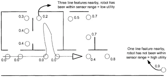
In order to evaluate how various approaches to observation planning improve the efficiency of exploration, we implemented and tested these approaches for one particular candidate identification and scoring method. Specifically, we used the Newman, Bosse, and Leonard candidate identification and scoring method, because it is the only method that can handle line feature maps. This candidate identification and scoring method places candidates at either end of a line feature, in order to encourage the robot to discover the full extent of the line. The method then estimates how much new area a robot will see from each candidate, by measuring the density of features around the candidate and seeing how closely the robot has passed by the candidate in the past. If there are many line features in the map around the candidate, then the robot must have seen the area around that candidate before. In addition, if the robot's path ever passed within sensor range of the area around the candidate, then it is also likely that the robot has seen that area before. The Newman, Bosse, and Leonard method summarize these measures of how much unexplored area a robot will see from a candidate into a utility and assigns this utility to the candidate. Figure 1.2 illustrates how the method places and scores candidates for a partially completed map. The triangle in the figure represents the robot's estimated position and heading. The line coming out of the back of the robot is the robot's estimated path through the environment. The circles represent candidates, and each candidate is labeled with its utility. The straight lines in the figure are the line features of the map.

Three line features nearby, robot has been within sensor range = low utility

0.30 0.2 0 0.5

Q

0.7

0.40

0.7

One line feature nearby,

robot has not been within

0.0 0.0 0.0 0.0 04 0.8 sensor range = high utility

F .62 Ide0ti Cadda 0 00 N 0 4t ,B ,

(16)

1.2 Approaches to Observation Planning

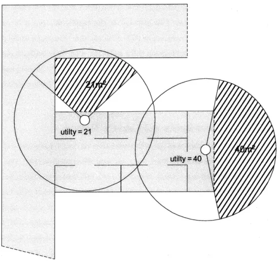
In order to evaluate how efficiently approaches to observation planning cause a robot to explore its environment, we must have some measure of the efficiency of the path that the robot executes during exploration. For now, we can measure the efficiency

of a robot's exploration by taking the sum of the utilities of the candidates that the robot visits before the robot's path exceeds a given maximum cost. The cost of a path may be the length of a path, the amount of time that it takes the robot to traverse the path, the amount of energy that the robot expends along the path, and so on. Because the utility of a candidate estimates how much new area the robot will see from that candidate, this measure quantifies the tradeoff between the desire to maximize the amount of new area that the robot maps, with the desire to minimize the cost of the robot's path.

Currently, all methods of exploring in order to increase map coverage take the greedy approach to observation planning. The greedy approach selects one candidate for the robot to visit, and outputs the least cost path to this candidate. The candidate that the greedy approach selects is the candidate that minimizes some function f(ci), where ci is a candidate'. One possible function is to return the cost of the least cost path to ci, in which case the greedy approach selects the candidate that the robot has the lowest least cost path to. Another possible function is to return the negative of the utility of ci, in which case the greedy approach selects the candidate that has the highest utility. Some

implementations combine the previous two functions by using a function that increases as the least cost path to ci increases and decreases as the utility of ci increases.

The problem with the greedy approach is that it only plans paths to be locally efficient. A series of locally efficient paths, however, is not guaranteed to be globally efficient. An obvious alternative to the greedy method, then, is to plan a globally optimal path. A globally optimal path is a path that takes the robot to every candidate in the map

' In the way it is described here, the greedy approach would more appropriately be named the myopic approach. Myopic decision making methods produce a one-step plan in which the agent takes the action that would be optimal if the agent's life were to end immediately afterwards. Greedy methods use the same criteria to choose actions to take as myopic methods, but greedy methods produce multiple step plans. Note, however, that a robot performing continuous observation planning with a myopic method would execute the exact same path as a robot performing continuous observation planning with a greedy method. In this thesis, therefore, we do not distinguish between these two methods. Instead, we use the term "greedy method" to refer both to methods that produce paths to only one candidate and to methods that produce paths to every candidate in the map greedily.

(17)

such that no other path taking the robot to every candidate has a lower total path cost. We call the observation planning method that outputs a globally optimal path for the set of candidates the full horizon method. We refer to paths planned by the full horizon approach as full horizon paths. Finding a globally optimal path for a given set of candidates maps to solving the Traveling Salesman Problem (TSP) over the set of candidates.2

If the robot is able to execute a full horizon path to completion without the set of

candidates changing at all, then the full horizon approach to observation planning is guaranteed to cause the robot to explore its environment at least as efficiently as any other observation planning method (as long as the maximum path cost, over which we measure efficiency, is not less than the cost of the full horizon path). Unfortunately, the set of candidates almost always changes as the robot explores its environment.

Candidates appear, disappear, move, and change utility as the robot finds out more about the environment, largely because most exploration methods place candidates on the border between the explored and unexplored parts of the map. As the robot increases the coverage of its map, this border moves outward, along with all of the candidates on the border. A robot performing continuous observation planning with the full horizon approach will recalculate the full horizon path to adjust for the set of candidates changing. However, if the robot does not get to execute its full horizon paths to

completion, then there is no guarantee that the parts of the full horizon paths that it does execute will be efficient at all.

In order to develop methods of planning efficient exploration paths when the set of candidates changes, we need to characterize the way in which the set of candidates changes. Unfortunately, there are currently no methods of predicting precisely how or when the set of candidates will change during exploration. However, we do know that the farther the robot travels, the more likely that the robot is to map previously unseen areas, and the more likely it is that the set of candidates will change. We, therefore, can model the times that the candidates change as an arrival-type stochastic process. Recall

2 Burgard et al [10] first pointed out that planning a globally optimal path to explore an environment maps

to solving the Traveling Salesman Problem. As far as we know, however, no one has ever implemented or evaluated a method of exploration for increasing map coverage that plans its paths by solving the TSP. The implementation and evaluation of the TSP approach for a particular candidate identification and scoring

(18)

that we can think of a stochastic process X[t] as a sequence of random variables, such that for any value of t = ti, X[ti] is a random variable. In an arrival-type stochastic

process, each random variable X[t] has two possible values: X[ti]= 1 (an arrival) or X[ti]

= 0 (no arrival). For our purposes, the variable t corresponds to the distance that the

robot has traveled, and an arrival corresponds to an instant when the set of candidates changes. We do not attempt to model how the set of candidates changes when it changes,

since how the set of candidates changes depends strongly on the particular candidate identification and scoring method.

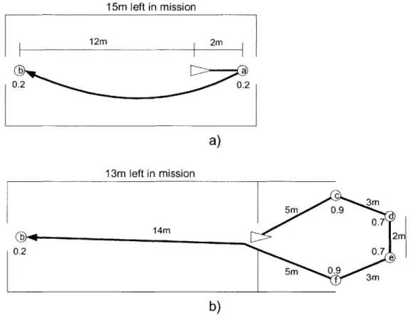
We can, therefore, think of an exploration mission as a series of intervals over which the candidates do not change. Each interval is separated from the interval before and after it by instants when the candidates change in an unpredictable way. With this model of how the candidates change, the best that an observation planning method can do is to plan paths that are optimally efficient over some distance in which the candidates are not likely to change. This distance could be any distance shorter than the longest interval over which the candidates do not change. A logical choice is the expected value of the distance between arrivals. To be precise, then, we would like the robot to plan a path that is not longer than a given distance (the horizon length) and that visits a subset of the candidates with the maximum possible total utility. We refer to this method of

observation planning as the finite horizon method. Finding such a path corresponds to solving the Selective Traveling Salesman Problem (S-TSP) over the set of candidates. The development and characterization of the finite horizon approach to observation planning is one of the main contributions of this thesis.

There are two reasonable choices for how to perform continuous observation planning using the finite horizon approach. First, every time we recalculate the finite horizon path, we can plan over the same horizon length, L. We call this method the

receding horizon method. Alternatively, each time the robot recalculates the finite horizon path, the robot can subtract from the horizon length, L, the distance it has traveled since the initial path computation and recalculate the path over this adjusted horizon. When L minus the distance traveled falls to zero, the robot resets its distance

traveled to zero and starts planning a path over a distance of L again. We refer to this method of re-computation as the fixed horizon method.

(19)

Neither finite horizon continuous observation planning method is clearly better than the other. A robot using the fixed horizon method is more likely to execute the paths it plans to completion without the set of candidates changing than a robot using the receding horizon method, for the length of the robot's plan constantly grows longer in the receding horizon method. Only when the robot executes its plan to completion without the set of candidates changing, can we guarantee that the robot will execute an efficient path. In other words, it is possible that the robot will constantly put off doing something

efficient when using the receding horizon method, and eventually the set of candidates will change so that the robot will never get to do the efficient thing it was planning on. Even though this situation is possible, however, it may not be likely. In addition, the fixed horizon method has the weakness that the planning horizon constantly gets shorter and shorter, thereby making the method more and more like the greedy approach. The receding horizon method, therefore, has the potential to plan much more efficient paths than the fixed horizon method.

Note that neither finite horizon continuous observation planning method plans globally optimal paths. Therefore, it is possible for a robot using the greedy or full horizon approach to execute a path that is more efficient than the path that a robot would execute using the finite horizon approach in the same situation. However, because the finite horizon approach plans a path that is optimally efficient over the expected distance that the robot will travel before the candidates change, we expect that the finite horizon approach will cause the robot to execute the most efficient paths on average. When the greedy or full horizon approaches cause the robot to explore more efficiently than the finite horizon approach, they must do so by getting lucky.

One legitimate concern about the finite horizon approach is that the robot might never be able to visit more than one candidate in its path before the set of candidates changes. In this case, there should not be any advantage on average to planning a path to multiple candidates, and the best the robot can do is use the greedy approach. This concern is legitimate because candidate identification and scoring methods intentionally place candidates in locations from which the robot is likely to map a lot of new area. And when the robot maps a new area, the set of candidates usually changes. Therefore, if

(20)

the candidate identification and scoring method is doing its job well, the set of candidates should change every time the robot makes an observation at a candidate.

This concern may mean that the finite horizon approach is not always the best approach to observation planning, yet there are situations in which the finite horizon approach should still perform better than the greedy (or full horizon) approach. For example, the first candidate in the robot's finite horizon path may usually not be much worse in terms of the greedy function than the greedily best candidate, depending on the environment. In these cases, if the robot is able to execute even just one of its finite horizon paths to completion, the robot still might explore its environment more

efficiently using the finite horizon approach than the greedy approach. In addition, we can shorten the length of the robot's horizon in order to make it more likely that the robot will be able to execute its finite horizon paths completely.

More importantly, there are situations in which the changes to the set of candidates do not usually affect the overall efficiency of a finite horizon path. These situations occur when the robot starts off knowing the large scale structure of the

environment and is mapping in order to fill in the details. If the robot knows where most of the large groups of obstacles and interesting areas to map are, then the robot can plan an efficient large scale path between these interesting areas. When the robot arrives at these areas, the robot will map new objects and the set of candidates will change, but these changes will usually only be local. The changes to the set of candidates will, therefore, not significantly affect the large scale shape and efficiency of the robot's planned path.

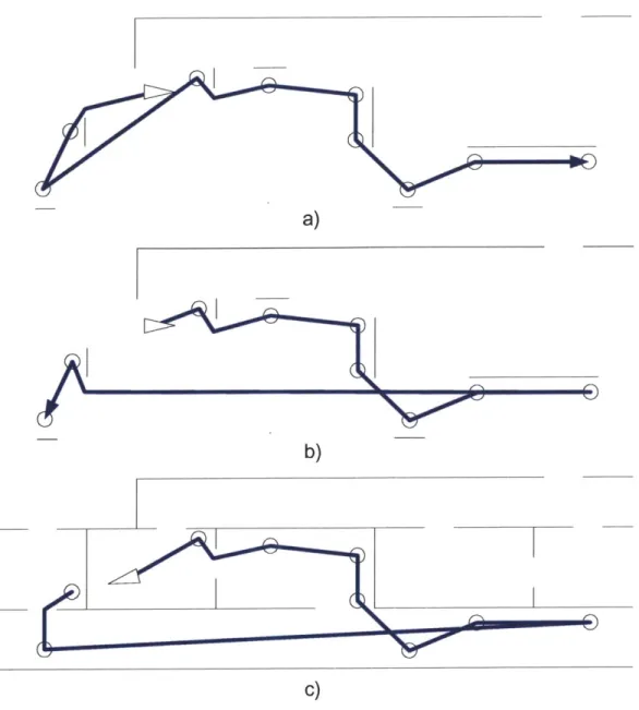
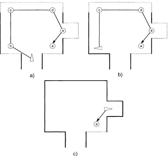
Figure 1.3 shows a simple example of such a situation. Figure 1.3a shows what the robot's environment actually looks like. The environment is a fictional Mars terrain,

and the squares represent rocks. The rocks are grouped into clusters, and the arrangement of these clusters is what we call the large scale structure of the environment. Figure 1.3b shows the robot's initial map. This map captures the overall structure of the

environment, in that we can discern the approximate location of each of the rock clusters. Figure 1.3c shows a path that the robot might plan using the finite horizon approach with

a long horizon. Note that even though the robot will discover new rocks and new candidates will appear that will change the robot's path at each cluster, the overall

(21)

structure of the robot's path will remain the same. Figure 1.3d shows the approximate path a robot might take to explore this environment using the greedy approach. Note that

the finite horizon path fills in the map in a much shorter distance than the greedy path.

O88o

00 0 D 0 00 0 D 11 03 o 0 0 0 a)

n

r r

r

-r-F-b) C) d)

Figure 1.3 Example of Knowing Large Scale Structure Beforehand

There are a number of ways in which the robot could start off knowing the overall structure of the environment. In some situations, it is easy for us to build large scale maps of an environment using low resolution sensors. We can then provide the robot with such a map a priori. For example, overhead satellite images can produce large scale maps of an environment in the case of Mars exploration. Such large scale maps do not

(22)

contain enough detail for the robot to use for navigation or path planning, however; therefore, the robot must explore in order to flesh out its map.

Another situation in which the robot starts off knowing some of the overall

structure of the environment occurs when the environment is open. An open environment is an environment in which the density of obstacles is low enough that, from most

positions, the robot can see most of its surroundings, out to the radius of its sensors. Although the robot will not start off knowing the structure of the entire environment, for open environments, the robot will know the structure of the environment out to the radius of its sensors. Then, if the robot plans its finite horizon paths over a horizon that is on the order of the length of this sensor radius, the robot should end up filling in the details of its map in parts of the environment for which it knows the basic structure. Therefore, we expect that changes to the set of candidates will not hurt the efficiency of a robot's finite horizon path in open environments.

Ultimately, however, in order to determine for certain in which situations the finite horizon approach outperforms the greedy and full horizon approaches, we must implement and test these approaches with particular candidate identification and scoring methods. Therefore, this thesis presents the results of testing these approaches with the Newman, Bosse, and Leonard candidate identification and scoring method.

1.3 Problem Statement

The problem that this thesis addresses is to design the greedy, full horizon, and finite horizon approaches to continuous observation planning, and evaluate their efficiency with respect to how efficiently a robot explores typical environments. Our approach to solving this problem breaks down into solving three sub-problems. First, we must implement these three approaches to continuous observation planning for a

particular candidate identification and scoring method, and test this implementation on typical environments. In order to solve this sub-problem, we also must address the problem of finding an efficient method of solving the S-TSP. Second, we must identify objective and quantifiable measures of how well a robot explores its environment. And third, we must evaluate how well these three approaches work for all candidate

(23)

identification and scoring methods, based on the features that candidate identification and scoring methods have in common.

1.4 Technical Challenges

Solving the sub-problem of implementing and testing the three approaches to continuous observation planning for a particular candidate identification and scoring method presents a number of technical challenges. First, performing continuous

observation planning using the full horizon or finite horizon approach is computationally difficult. In order to perform continuous observation planning with either of these two approaches, the robot must constantly find the least cost path that avoids obstacles between each pair of candidates, and then solve the TSP or S-TSP over the set of candidates using these least cost paths. Because the autonomous exploration

implementation must control a robot in real time, the duration of the path planning and

TSP or S-TSP solving stages must be on the order of seconds at most.

The fact that our implementation uses line feature maps as the map representation presents another challenge. As far as we know, there are no existing methods of planning least cost paths that avoid obstacles using a line feature map. Therefore, we must

develop a principled, effective, and efficient method of path planning for line feature maps. Another challenge in implementing these observation planning methods is that the

S-TSP is an NP-hard problem [30]. Therefore, finding a fast method of solving the

instances of the S-TSP we are likely to encounter has the potential to be very difficult. One final challenge that we face is that few if any researchers have attempted to measure quantitatively how well a robot explores its environment in order to increase the coverage of its map. Therefore, must develop reasonable and objective methods to quantify the quality of a robot's exploration.

1.5 Technical Approach

Recall that, in order to evaluate the performance of the greedy, full horizon, and finite horizon approaches to observation planning, we implemented these three

approaches for the Newman, Bosse, and Leonard candidate identification and scoring method described in Section 1.1. We then used the implementation of these observation

(24)

planning approaches to control a robot's exploration of indoor and outdoor environments in simulation and in the real world. This implementation and the experiments we

performed with it are important contributions of this thesis.

Specifically, we put together an experimental system that continuously takes as input, real or simulated sensor data, builds a line feature map from this data, and outputs commands to a real or simulated robot that causes the robot to explore its environment using a specific observation planning method. The continuous observation planning methods we implemented were a greedy method, the full horizon method, the receding horizon method, and the fixed horizon method. Our implemented greedy method selects to visit the candidate to which the robot has the lowest least-cost path.

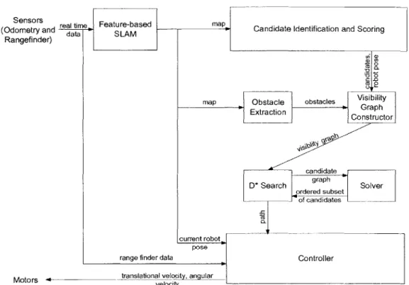
Figure 1.4 shows the architecture of the experimental system. The system is structured so that the only module that changes when we switch to using a different observation planning method is the module labeled "solver." The solver module takes as input a graph with one vertex for each candidate, one vertex for the robot, and edges with weights equal to the cost of the least cost path through the robot's map between the endpoints of the edge. We refer to such a graph as a candidate graph. The solver module outputs a sequence of candidates for the robot to visit. The system then turns this

sequence into a path for the robot to execute. We first describe all of the modules except the solver module. We then explain how we constructed the full horizon and finite horizon versions of the solver module.

(25)

(Odometrsand real time _{(Ooreryad edata} Feature-based _SLAM mapl Candidate Identification and Scoring Rangefinder)

Figure 1.4DArchtecture ofeExprimental Syste

1.5.1ndd Ore a

u Te fe Secnto tae omte rbt

finder. data t datin tremapoh

toMtheandit dentif o anscing odnule

TheFcadideigen i crig m le sste Nwan, Bose

Leonard methd dsrie tiond peneteatobseti

frmaWie fexature map. mTdhes canithe arieplaced dcoedto encurage. afrobonpt to expndets aprangede. The module esef cidate to pte artiem of the stem

environment and to estimate the rob curt's p ritobintema.Fge.shwatyia

pefors pa pe t potrogee

Tateof tant seormns liodg n epulae

Theadidateiei1.ai4 Andhicuring Epmetale Ss temNwaBsen

1e.5 eho ecie i eto .1 Ovgeerale arcisetur of andiaeembseration pit frmaWie fexature map. Thdeso adte ariecptaredepantd ine tFigurae a frobnpt to extpanuta. Thtr-e d SLAsse mohue ecofnidaesl tktes at fof the sytsmha

odmte adrangfiner yTemodl huserers pth paann tods a lineatur masp oat th

avoids obstacles between each pair of candidates, in order to build the candidate graph. To find these least cost paths, the system builds a visibility graph over the current map and the set of candidates [51]. The module labeled "visibility graph constructor" in

(26)

Figure 1.4 builds the visibility graph from a set of polygonal obstacles and a set of waypoints. The corners of the obstacles and the waypoints make up the vertices of the visibility graph. The visibility graph constructor places edges between every pair of vertices such that the edge does not pass through an obstacle. The cost of the edge is the straight line distance between the two vertices. Therefore, any path formed by traversing edges in the graph from one vertex to another is guaranteed to avoid all known obstacles. In order to find the least cost path through the map between any two candidates, the system searches the visibility graph for the least cost path between the corresponding vertices.

The system uses the information in the line feature map to provide the visibility graph constructor with a set of polygonal obstacles. This thesis presents a novel method of extracting a set of obstacles from a line feature map, by turning each line in the map into a rectangle. The module labeled "obstacle extraction" in Figure 1.4 builds these rectangles from the feature map.

The system uses the D* algorithm [45] in order to search the visibility graph for the least cost path between every pair of candidates. As we note in Section 1.4, it is computationally challenging to constantly search the visibility graph for these shortest paths. D* addresses this challenge by incrementally searching graphs. In other words,

D* saves its last calculated set of least cost paths. Then, when the map updates and a

new visibility graph is built, the system tells D* what edges changed in the visibility graph. D* then searches the visibility graph only as much as it needs, in order to update its saved set of least cost paths, to accurately reflect the least cost paths through the visibility graph between every pair of candidates. The module labeled "D* search" in Figure 1.4 performs this incremental search and creates the candidate graph. The D*

search module then passes the candidate graph to the solver module. The solver module returns an ordered subset of candidates to visit. The D* search module uses its stored set of least cost paths to fill in the path between these candidates. The D* search module then passes this path to the module labeled "controller" in Figure 1.4.

The controller module takes a path as input and outputs commands that cause the robot to follow this path. The controller module also performs low level obstacle

(27)

In order to perform this obstacle avoidance, the controller module continuously reads the rangefinder sensor data.

1.5.2 The Solver Module

The solver module takes a candidate graph as input and outputs an ordered subset of candidates to visit. There are four versions of the solver module: the greedy version, the full horizon version, the receding horizon version, and the fixed horizon version. The greedy version simply searches through all of the edges leading out of the vertex

representing the robot for the edge with the lowest weight and returns the candidate at the other end of this edge. The full horizon version solves the TSP on the candidate graph and returns the resulting sequence of candidates. The receding horizon version solves the

S-TSP on the candidate graph for the constant horizon length L and returns the resulting

ordered subset of candidates. The fixed horizon version solves the S-TSP on the candidate graph for a horizon length of L-d, where L is a constant and d is the distance the robot has traveled since the last horizon, and returns the resulting ordered subset of candidates.

We use the Concorde TSP code [54] directly to solve the TSP. Concorde implements an efficient branch-and-cut algorithm [1] for solving the TSP on undirected graphs. Instead of using existing algorithms to solve the S-TSP, however, we developed and implemented a new approach. In order to solve the S-TSP, we formulate the problem as an Optimal Constraint Satisfaction Problem (OCSP) [50]. An OCSP consists of a set of variables with finite domains, a set of constraints which map each assignment to the variables to true or false, and a utility function that maps each assignment to the variables to a real number. A solution to an OCSP is an assignment to the variables that maximizes the utility function such that the constraints are satisfied. A major reason that we

developed an approach to solving the S-TSP by formulating it as an OCSP is that this formulation has not been previously explained. Powerful methods of solving OCSP's have recently emerged [50]; therefore, it is worthwhile to see how well these methods work for the instances of the S-TSP we are interested in.

In order to formulate the S-TSP as an OCSP, we create one variable for each candidate. Each variable can take the value of either I or 0. The candidate

(28)

corresponding to a variable that is assigned to 1 is included in the ordered subset of candidates that is the solution to the S-TSP, while the candidate corresponding to a variable assigned to 0 is not included. Each variable also has its own utility function, which we call an attribute utility function. This function maps a variable assigned to I to the utility of the corresponding candidate and a variable assigned to 0 to zero. The utility of an assignment to the entire set of variables is equal to the sum of the values of the attribute utility functions of the individual variables. In order to describe the constraint, let us consider the sub-graph formed by removing every vertex corresponding to a candidate whose variable is assigned to 0 (and every edge including such a vertex) from the candidate graph. The constraint over the OCSP variables is that the solution to the

TSP on this sub-graph must have a length that is less than or equal to the horizon length

L.

We solve the S-TSP formulated as an OCSP with the constraint-based A* algorithm [50]. Constraint-based A* is an efficient method based on A* search of

enumerating the possible assignments to the variables from highest to lowest value of the utility function. Note that in order to maximize the utility function for a partial

assignment to the variables, it is sufficient to assign each of the unassigned variables to a value that maximizes its attribute utility function. Constraint-based A* takes advantage of this fact in order to efficiently find the next best full assignment to the variables, and in order to efficiently calculate an admissible heuristic during the search.

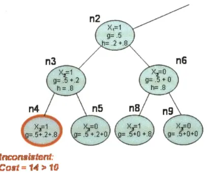
In order to solve the S-TSP, constraint-based A* enumerates full assignments to the variables one at a time and checks the constraint for each assignment. Our approach checks the constraint on an assignment by running the Concorde TSP solver on the sub-graph corresponding to the assignment. The first full assignment that constraint-based

A* finds is consistent must correspond to the subset of candidates in the solution to the S-TSP, since these assignments are generated in best first order. In order to turn this subset

of candidates into an ordered subset, our approach orders the candidates in the subset in the same order that the TSP solver outputted.

(29)

1.6 Thesis Claims

1. When a robot knows the large scale structure of its environment early on

during exploration for increasing map coverage, the finite horizon approach to

observation planning will cause the robot to explore this environment more efficiently on average than either the greedy or the full horizon approach.

2. It is possible to solve the S-TSP as an OCSP using the constraint-based A* algorithm.

1.7 Thesis Layout

The rest of this thesis is laid out as follows. Chapter 2 characterizes the problem of autonomous exploration and provides background on map representations, existing approaches to exploration for decreasing map uncertainty, and existing approaches to exploration for increasing map coverage. In particular, the chapter describes in detail the Newman, Bosse, and Leonard candidate identification and scoring method that the implementation we tested uses. Next, Chapter 3 characterizes the general features of observation planning and motivates and defines the finite horizon approach. Chapter 3 also speculates about how well the greedy, full horizon, and finite horizon approaches should perform for all candidate identification and scoring methods in general by looking at the features that all candidate identification and scoring methods share. Chapter 4 describes in detail our approach to solving the S-TSP as an OCSP with constraint-based

A*. Then, Chapter 5 explains the architecture of the system that we implemented to test the greedy, full horizon, and finite horizon approaches to observation planning. Chapter

6 presents and analyzes the results of testing the system we implemented in real and

simulated environments. Finally, Chapter 7 discusses ideas for future work in areas touched upon by this thesis.

(30)

2 Autonomous Exploration

In this chapter we formulate the problem of autonomous exploration and give an overview of some of the methods for solving the problem that researchers have pursued. Finally, we describe in detail the method of exploration that the system we tested in our experiments is based on.

Specifically, in Section 2.1 we define the problem of exploration and introduce the two major variations of the problem: exploration for increasing map coverage and exploration for decreasing map uncertainty. In Section 2.1.2 we describe the general structure of an exploration algorithm that virtually all algorithms use. In Section 2.2 we review a number of the common approaches to building maps that exploration algorithms use, including the feature-based SLAM approach that the exploration algorithm we tested uses. Then, in Section 2.3, we characterize the problem of exploring in order to increase map coverage and describe a few important approaches to this type of exploration out of the many that exist. In Section 2.3.4 we describe the feature-based exploration strategy that we based the system that we tested on. Finally, in Section 2.4, we characterize exploration for decreasing map uncertainty and go over a few approaches to this type of exploration.

2.1 The Problem of Exploration

Being able to autonomously explore an environment in order to construct a map of this environment is integral to mobile robotics [10] [37] [22]. Most tasks that a mobile

robot might have to perform, such as taking samples of rocks on Mars, locating ocean mines, performing urban search and rescue, or simply traveling from one location to

another, require the robot to be able to navigate accurately. Yet in many environments, including indoors, underwater, or on Mars, GPS is not available to help. In addition, the odometry error for many robots is unacceptable and accumulates over time. As a result, the best way for a robot to navigate is often to use its sensors to localize itself within a

(31)

map of the surroundings. A map also functions as a model of the environment that the robot can use for path planning.

The main issue with relying on maps is that we often do not have an a priori map of the environment to give to the robot. Fortunately, algorithms now exist [38] [8] that enable a robot to use its sensors to build a map of its environment and at the same time localize itself within this map, all in real time. These algorithms are known as

simultaneous localization and mapping (SLAM) algorithms. We discuss approaches to

SLAM in Section 2.2.

SLAM algorithms, however, only solve part of the problem of building a map of

an environment. A SLAM algorithm passively takes what the robot's sensors see and builds the best map possible from this data; it does not direct the robot to sense new areas of the environment. A robot can attempt to build its map as it moves around performing its other tasks, yet often this type of haphazard exploration of the robot's surroundings leads to an inadequate model of the environment. Therefore, we would like the robot to be able to drive itself around an environment before it performs its other tasks in order to build a good map of that environment. We call driving about for the purpose of building a map autonomous exploration.

2.1.1 Definition of the Problem of Autonomous Exploration

In order to be clear about what autonomous exploration algorithms do, we define the problem of autonomous exploration more formally. Given a partially completed map that is constantly updated to reflect the robot's sensor readings and the robot's estimated position, the problem ofautonomous exploration is to have the robot control itself in order to improve this map. We explain the terms in this definition below.

By a "partially completed map," we simply mean a map that does not model

every object in the robot's environment with one hundred percent accuracy. All map building algorithms output partially completed maps.

There are a number of ways that a robot can "control itself' while exploring. Some sensors allow the robot to control where and when they sense. For example, scanning sonar sensors can be told to take readings at certain angles and certain times

(32)

computational burden of processing this data on the robot. Yet in many robot setups, the sensors constantly scan the environment at all possible angles, and therefore the only thing the robot can control is where the robot drives to. Thus, most of the exploration algorithms we examine in this chapter only consider how to drive the robot during exploration.

Finally, there are two main ways a robot can "improve" its map of the

environment: by decreasing the uncertainty in the map and by increasing the coverage of the map. A robot's sensors are inevitably noisy; therefore, SLAM algorithms represent the locations of objects in their maps with joint probability density functions. In order to decrease the uncertainty in its SLAM map, a robot must re-observe the objects in the environment that it has already mapped in such a way as to narrow the joint pdf over the locations of these objects in the map. The more focused the joint pdf is, the more certain the robot is about where the objects are located.

Conversely, in order to increase the coverage of its map, a robot must map objects and regions that it has never seen before. Therefore, these two aspects of improving a map compete. We examine methods of exploring to decrease map uncertainty and methods of exploring to increase map coverage in separate sections. Nevertheless, many exploration algorithms try to find an acceptable balance between these two ways of improving a map.

Now that we understand the requirements of the problem of exploration, we can make some general statements about how algorithms approach this problem.

2.1.2 General Features of Exploration Methods

As we have already noted, most approaches to autonomous exploration assume that the robot's sensors are constantly scanning their full range; therefore, the robot can

only control how it drives around its environment. Most exploration methods deal with controlling the robot's driving by breaking down the problem into two sub-problems. The first sub-problem is to plan a path for the robot to execute that will improve the map, and the second sub-problem is to send the commands to the hardware to cause the robot to execute this path. The first sub-problem is where most of the interesting variation between exploration methods occurs, and we call it the exploration path planning

(33)

problem. More precisely, given a partially completed map and the robot's estimated position within the map, the exploration path planning problem is to output a path that the robot can use to effectively control its motion in order improve the map.

The simplest way for the robot to explore using this approach is to fully solve the exploration path planning problem and then execute the resulting path completely. Once the robot has executed the path to completion, it begins the loop over and solves the exploration path planning problem again. The pseudo-code in Figure 2.1 depicts this exploration method. The function MissionCompleted () on line I of Figure 2.1 returns true if the exploration mission has finished. The mission might be set to last either until the robot travels a set distance, until a certain amount of time passes, or until the user sends a command to halt the exploration. The function

GetMost_RecentMap (constantly updating map) takes a dynamic map, which a map building algorithm is constantly updating, and returns a static map that reflects the most recent state of the dynamic map. Because SLAM algorithms include the robot as part of the map, the function GetCurrentRobotPose (map) can take this static map and return the location of the robot.

Explore(constantly updating map) returns nothing

1. while MissionCompleted() is false

2. let map = GetMostRecent_Map(constantly

updating map)

3. let robot pose = GetCurrentRobotPose(map)

4. let path = PlanExplorationPath(map, robot

pose)

5. ExecutePath(path)

6. endwhile

Figure 2.1 Pseudo-code for Exploration using Basic Exploration Path Planning

The problem with this method of exploration is that the map is very likely to change as the robot executes the path it has planned. And if the map changes, the path might become sub-optimal or even impossible to execute. Therefore, another possible method of exploration is to periodically halt the execution of the path and solve the