Turbulent separation upstream of a forward-facing step

(1)

Turbulent separation upstream of a

forward-facing step

D. S. Pearson1,_†_{, P. J. Goulart}1,2 _{and B. Ganapathisubramani}1,3 1_{Department of Aeronautics, Imperial College London, London SW7 2AZ, UK}

2_{Automatic Control Laboratory, ETH Z¨urich, 8092 Z¨urich, Switzerland}

3_{Aerodynamics and Flight Mechanics Group, University of Southampton, Southampton SO17 1BJ, UK}

(Received 4 June 2012; revised 22 December 2012; accepted 19 February 2013; first published online 29 April 2013)

The turbulent flow over a forward-facing step is studied using two-dimensional time-resolved particle image velocimetry. The structure and behaviour of the separation region in front of the step is investigated using conditional averages based on the area of reverse flow present. The relation between the position of the upstream separation and the two-dimensional shape of the separation region is presented. It is shown that when of ‘closed’ form, the separation region can become unstable resulting in the ejection of fluid over the corner of the step. The separation region is shown to grow simultaneously in both the wall-normal and streamwise directions, to a point where the maximum extent of the upstream position of separation is limited by the accompanying transfer of mass over the step corner. The conditional averages are traced backwards in time to identify the average behaviour of the boundary-layer displacement thickness leading up to such events. It is shown that these ejections are preceded by the convection of low-velocity regions from upstream, resulting in a three-dimensional interaction within the separation region. The size of the low-velocity regions, and the time scale at which the separation region fluctuates, is shown to be consistent with the large boundary layer structures observed in the literature. Instances of a highly suppressed separation region are accompanied by a steady increase in velocity in the upstream boundary layer.

Key words: boundary layer separation, turbulent boundary layers

1. Introduction

The flow of an incompressible boundary layer over a forward-facing step produces dynamic behaviour of considerable complexity. The flow creates regions of mean deceleration, acceleration, separation, reverse flow and reattachment. It produces two regions of separation: one upstream and one downstream of the step face. Both separations are subject to continuous buffeting from the surrounding flow and are highly unsteady. This unsteadiness causes large pressure fluctuations on the step surfaces (Efimstov et al. 2002; Largeau & Moriniere2007; Camussi et al.2008) and is a source of drag, pressure loss (Moss & Baker1980) and noise (Ji & Wang 2010). The

† Email address for correspondence:d.pearson08@imperial.ac.uk

https:/www.cambridge.org/core

. University of Basel Library

, on

30 May 2017 at 13:57:45

, subject to the Cambridge Core terms of use, available at

https:/www.cambridge.org/core/terms

.

(2)

aim of this study is to examine the characteristics of the upstream separation region and the physical mechanisms that contribute to its unsteadiness.

The majority of published literature on the forward-facing step focuses on the flow downstream of the step face. In particular, previous work has concentrated on the factors affecting the streamwise position of the downstream reattachment xr as well as wall-pressure fluctuations within this reattachment region. Initial work by Mohsen (1967) demonstrated that xr was a stronger function of step height than Reynolds number, and Arie et al. (1975) showed how the pressure signature varied over steps of varying streamwise extent. Moss & Baker (1980) provided a detailed examination of the mean downstream separation using pulsed wire anemometry, showing the dramatic increase in separation size and reverse flow velocity for steps of streamwise extent less than xr. The experimental measurements of Camussi et al. (2008) identified the downstream recirculation as also being the location of maximum root mean square (r.m.s.) wall pressure and showed an increase in the power of fluctuations at low frequencies, approximately StL= fL/h = 0.2. The same effect was shown by Largeau & Moriniere (2007) who attributed these dominant frequencies to a flapping of the point of reattachment caused by large structures in the separation region. These similarities show that the processes governing the separation region are similar despite the xr being different in each study: xr/h = 3.2 (Leclercq et al. 2001), 1.5–2.0 (Camussi et al. 2008) and 4_{.5–5 (Largeau & Moriniere} 2007). Such is the sensitivity of xr to the flow field parameters such as Re and δ/h, no consensus on specific dependencies has been reached: a point succinctly summarized by Sherry, Lo Jacono & Sheridan (2010) and reiterated by Hattori & Nagano (2010).

Conversely, the position of the upstream separation xsep has been consistently measured to lie between −0.8h and −1.2h (Moss & Baker 1980; Leclercq et al.

2001; Largeau & Moriniere 2007; Addad et al. 2003; Camussi et al. 2008; Marino & Luchini 2009) thereby only showing weak dependence on the flow field parameters. It is likely that the flapping of the downstream separation shear layer, and hence the turbulent stresses and acoustic emission that result, are influenced to some degree by the upstream flow. This study seeks to provide insight into the upstream flow mechanisms of the forward-facing step configuration. Which, while of interest in its own right, will also contribute to an understanding of the flow conditions imposed on the downstream separation.

Some features of the upstream separation were identified in the oil-film and laser-sheet visualizations by Martinuzzi & Tropea (1993). In particular they showed that the spanwise extent of the step is crucial in defining its characteristics. They showed that as the spanwise extent increases, the edge effects of the finite span reduce, while a system of saddle and nodal points develops on the step face. The same patterns were identified by St¨uer, Gyr & Kinzelbach (1999) using hydrogen bubble visualization, who then used particle tracking velocimetry (PTV) to demonstrate the dynamic processes responsible. They found that the upstream separation contains systems of vortex structures that travel spanwise along the bottom corner of the step. These vortices are shown to occasionally grow so large they are released as streaks of fluid over the top of the step. This ejection of mass over the step also occurs with apparent spanwise spatial periodicity, explaining the node and saddle points observed by Martinuzzi & Tropea (1993). These findings were confirmed numerically by the work of Wilhelm, Hartel & Kleiser (2003), which showed remarkable agreement with St¨uer et al. (1999) in the motion of the streaks over step corner. The simulations also followed these streaks downstream to show that they roll up into pairs of counter-rotating vortices that propagate past the region of downstream separation,

, on

30 May 2017 at 13:57:45

.

(3)

thereby proving a direct interaction between the upstream and downstream separation regions. In the studies of both St¨uer et al. (1999) and Wilhelm et al. (2003) the flow approaching the step was laminar. This allowed them to perform linear stability analysis and to show that the corner vortices were not an absolute instability, rather a sensitive reaction to the upstream perturbations.

The issue of flow stability and the sensitivity of the separation regions to upstream perturbations was recently addressed in the numerical studies of Lanzerstorfer & Kuhlmann (2012) and Marino & Luchini (2009). These two studies broadly support the assertion of Wilhelm et al. (2003) that the instabilities are a result of upstream perturbations, despite highlighting discrepancies of the critical Reynolds number for absolute instability. In particular, this topic is discussed in detail by Lanzerstorfer & Kuhlmann (2012).

The presence of fluid streaks over the step corner is evidence of a mechanism by which the upstream separation influences the downstream one. To date, neither this, nor the role of perturbations in the oncoming boundary layer, has been identified for the turbulent case. Understanding, estimating and perhaps eventually controlling this transfer of mass over the step will enable the detrimental effects of the high-pressure fluctuations at the downstream reattachment point to be mitigated. Finding the upstream conditions that precede such events in a turbulent flow will allow progress towards this goal.

The current study presents experimental evidence for the relation between fluctuations in the upstream boundary layer and the structure of the separation region upstream of the forward-facing step. The experiment is introduced in §2, followed by a statistical description of the shape and size of the separation using conditional averages in §3. The relation between extreme separation events and the upstream boundary layer is shown in §4. The conclusions of this work are presented in §5.

2. Experimental data

The experiments are conducted at Imperial College London in a low-speed recirculating wind tunnel that has a working section 1370 mm wide, 1120 mm high and 2980 mm long. The tunnel has optical access from one side. A forward-facing step of height h = 30 mm is placed on the tunnel floor perpendicular to the flow. The step covers the entire spanwise extent of the working section and extends x_{/h = 33} downstream. The boundary layer is tripped using a sandpaper strip at x_{/h = −62 to} ensure the boundary layer at the step face is fully turbulent. The free-stream velocity was set at U_∞_{= 10 m s}−1_.

Two-dimensional high-speed particle image velocimetry (PIV) measurements are taken in the wall-normal plane, parallel to the flow direction, at the spanwise centreline. The light from the laser enters the wind tunnel through a small aperture in the wall before being reflected downward and spread into a sheet. The mirror and light sheet optics are mounted on a three-axis traverse, enabling precise adjustments of the light sheet position and orientation. Two Phantom V12 1280 × 800 pixel resolution CMOS cameras are aligned side by side, each fitted with a Sigma 105 mm f_/2.8 macro lens. Figure 1(a) shows a schematic representation of the PIV arrangement and figure 1(b) shows the field of view of each camera. The two cavities of a Litron LDy353 Nd:yLF laser are fired simultaneously at 8000 Hz. The memory capacity of the two cameras allows a series of 31 606 images to be stored, which are used to calculate 31 605 time-resolved vector fields. The PIV field of view covers a streamwise

, on

30 May 2017 at 13:57:45

.

(4)

1.0 0.5 1.5 –5 –4 –3 –2 –1 0 0.2 0.4 0.6 0.8 1.0 –5 –6 –4 –3 –2 –1 0

PIV camera 2 field PIV camera 1 field

Traverse system

Mirror and light sheet optics Laser Camera 2 Camera 1 (c) (b) (a)

FIGURE1. (a) Schematic representation of the PIV arrangement. (b) The camera field of view and coordinate system. (c) PIV mean streamwise velocity U with streamlines shown. distance of approximately 5.5 h upstream of the step as shown in figure 1(b). The vector fields are processed using the LaVision DaVis software with a final window size of 16 × 16 pixels (with 50 % overlap). This results in a spatial resolution of approximately 1.1 mm (h/27) in both streamwise and wall-normal directions. The instantaneous velocity components in the streamwise–wall-normal directions (x, y) calculated from the PIV data are denoted as (U, V), with the mean and fluctuating velocity components as (U, V) and (u0_{, v}0_{), respectively. Figure}₁_{(c) shows the contours} of a mean streamwise velocity field with selected streamlines showing the mean size and shape of the recirculation region upstream of the step.

The oncoming boundary layer is characterized using a Dantec MiniCTA constant-temperature hotwire anemometer. A 5 µm wire probe is mounted to the tunnel traverse system and is moved in the wall-normal direction with a resolution of 6_{.25 µm.} The hotwire data is sampled at 20 kHz and low-pass filtered at 10 kHz. The probe is calibrated beside a Pitot tube in the free stream, with the differential pressure measured in Pascals to an accuracy of two decimal places using a Furness Controls

, on

30 May 2017 at 13:57:45

.

(5)

5 10 15 20 25 30 0 101 ₁₀2 ₁₀3 100 ₁₀4

Hotwire (no step)

FIGURE 2. Boundary-layer profile with and without the step. The presence of the step shortens the wall-normal extent of the log region. The PIV measurements are shown to be in good agreement with those from a hotwire. The minimum wall-normal extent of the PIV data is y+_{≈ 50.}

FCO510. Figure 2 shows the boundary layer profile with and without the step present. The quantities are normalized using mean skin-friction velocity, U_τ (determined using the Clauser chart method with log-law constants of _{κ = 0.41 and C = 5), and} kinematic viscosity, _{ν, denoted with superscript ‘}+_{’. The incoming boundary layer (i.e.} the boundary layer at a streamwise location that is not affected by the presence of the step, or alternatively the boundary layer with the step removed) has a 99 % boundary layer thickness of _{δ = 44 mm, displacement thickness of δ}∗ _{= 5.7 mm, momentum} thickness of _{θ = 4.2 mm and a U}_τ _{= 0.42 m s}−1_{. In the presence of the step at a} streamwise location of x = −5.2h, the boundary layer friction velocity drops to the value U_τ_{= 0.33 m s}−1_{. The boundary layer profile obtained using PIV measurements} under the same conditions is also shown in figure 2 for comparison, with the closest data point to the wall at y+_{≈ 50. The PIV and hotwire data are in close agreement} and both show an enlarged wake region typical of flow in an adverse pressure gradient.

It is well understood that the δ/h ratio plays a role in the flow dynamics over a forward-facing step (Sherry et al. 2010). To investigate the interaction of the oncoming boundary layer and the upstream separation, it is advantageous to ensure that the scale of boundary layer perturbations is large in comparison to those of the upstream separation. For this reason, a step submerged in the boundary layer, with a ratio of δ/h = 1.47, is investigated. Indeed, the major studies investigating the stability of the forward-facing step (St¨uer et al. 1999; Wilhelm et al. 2003; Marino & Luchini 2009; Lanzerstorfer & Kuhlmann 2012), have all used channel flow configurations, i.e. with effective_{δ/h > 1.}

The Reynolds number of the flow is Reh = 20 000 based on step height or Re_θ= 2800 based on the boundary-layer momentum thickness. The experiment was conducted at the largest practicable Reynolds number for which the time-resolved PIV data could be acquired (at sufficient frequency and spatial resolution for the required field of view). The Reh of the present data is of the same order as many of the

, on

30 May 2017 at 13:57:45

.

(6)

102 ₁₀3 f (Hz) 101 ₁₀4 10–8 10–6 10–4 10–2 2 kHz filter TRPIV Hotwire [–1.0, 0.5] [–2.0, 0.5] [–3.0, 0.5] [–4.0, 0.5] [–5.2, 0.5] [–5.2, 0.5]

FIGURE 3. Frequency spectra of PIV and hotwire measurements in the presence of the step. The PIV spectra are shown at various streamwise locations. All locations show a common noise floor at frequencies higher than approximately 1–2 kHz. A 2 kHz lowpass filter was used to remove the noise from the PIV data without loss of flow information.

experimental studies discussed in §1, thereby allowing the results to be interpreted in the context of existing publications.

Figure3shows the spectra of the PIV velocity data at different streamwise positions and y_{/h = 0.5. As the flow approaches the step, there is an increase in the low} frequency energy. The spectra also show that the noise floor in the PIV data is similar at all locations and occurs at a frequency of approximately 2 kHz. This frequency corresponds to a time scale of 3.5 wall-units (i.e. f+_{= f ν/U}2

τ≈ 0.285). There is very little energy at these frequencies, which is evident from the fact that this noise floor is over three orders of magnitude below the most energetic velocity fluctuations. In order to remove the effects of this noise from the data, the time-resolved data is low-pass filtered at a frequency of 2 kHz and since there is very little energy at these frequencies the filtering can be performed without loss of information. Also shown in figure 3is the hotwire spectra at x_{/h = −5.2 and y/h = 0.5. The hotwire and PIV data} are in good agreement overall, but the PIV spectra shows slight attenuation at high frequencies. This is due to the poorer spatial resolution of the PIV data compared with that of the hotwire. The hotwire data has a noise floor of lower magnitude than the PIV data, starting at frequencies of approximately 4–5 kHz.

Figure 4(a) and (b) show an example of the u0 _and _v0 _{velocity field perturbations} respectively. In figure 4(a) the inclined structures of the boundary layer are visible, with magnitude approximately ±0.2U∞. The v0 perturbations of figure 4(b) and the u0 _{perturbations of figure} ₄_{(a) are typically opposite in sign across the flow domain.} This is commonly observed for a convecting turbulent boundary layer and indicates the presence of ejections and sweeps in the wall region (Corino & Brodkey 1969; Willmarth & Lu1972).

It is the objective of the current work to investigate the perturbations of the boundary layer and their effect on the shape and size of the separation region in the step corner. Inspection of streamline patterns, such as those in figure 1(c), is the best method of determining the shape and size of the separation. However, for turbulent flows, the streamlines are unsteady and appear meandering at any instant,

, on

30 May 2017 at 13:57:45

.

(7)

(a) 0 0.2 0.4 0.6 0.8 1.0 1.0 0.5 1.5 –5 –4 –3 –2 –1 (b) 1.0 0.5 1.5 –5 –4 –3 –2 –1 (c) 1.0 0.5 1.5 –5 –4 –3 –2 –1 –0.15 –0.07 0 0.07 0.15 –0.10 –0.05 0 0.05 0.10 U < 0

FIGURE4. An example PIV vector field. (a) Streamwise velocity perturbations u0. (b) Wall-normal velocity perturbations_v0_{. (c) Streamwise velocity U with region of reverse flow}

shown.

making an unambiguous assessment of separation size as a function of time difficult. A feature of the present experiment is that reverse flow, i.e. U< 0, only occurs within the separation region. Therefore, the total area of reverse flow, A0, present in any vector field is a useful measure of the degree of separation present and, since it is readily calculated at each time instant, is a suitable quantity to study in the present analysis. Figure 4(c) shows the streamwise velocity of same PIV field with the bounding contour of U _{< 0 included. In this example the area enclosed by this} contour is a single region with area A0/h2= 0.07. In general, the reverse flow may be distributed in small disjoint regions within the vicinity of the step face. Under these circumstances, A0 is taken to be the sum of all regions of U< 0.

The analysis presented in the following sections is based on the varying magnitude of reverse flow with time A0(t). Of interest is how A0 relates to the wider flow field and, in particular, the shape and size of the region of separation.

3. Area of reverse flow and separation region

In order to investigate the structure of the separation and its response to upstream perturbations, instances of similar flow behaviour are isolated to allow observations of the average flow behaviour. The conditional averaging method is used for this purpose

, on

30 May 2017 at 13:57:45

.

(8)

0 0.005 0.010 0.015 10–1 10–2 ₁₀0

FIGURE5. Power spectral density premultiplied by frequency for the streamwise centroid of reverse flow. A broad peak in power is shown at St ≈ 0.09.

as it represents the best nonlinear estimate of a quantity with respect to some given event criteria (Adrian & Moin 1988). The choice of event over which the average is taken needs to be quantitative and relevant. As described in §2, for the study of separated regions, a valid choice of criteria is the total area of reverse flow present at any instant.

For a velocity field with components U(x, y, t) and V(x, y, t) over a two-dimensional PIV field of viewΩ, we define the area of reverse flow as

A0(t) = Z

ΩH (U(x, y, t)) dx dy.

(3.1)

H (p) =(0, p > 0₁_{, p < 0.} (3.2) The set of all time instants T for which the normalized area of reverse flow A0(t)/h2 has a value between two scalar limits [a, b] can then be expressed as

T_[a,b]_{= {t | a < A}0(t)/h2< b}, (3.3) from which it follows that the conditional average of all t ∈ T[a,b] is

hU (t)it∈T[a,b], (3.4)

where h·i denotes the ensemble average computed over all PIV fields that satisfy the given condition. The conditional quantity of (3.4) is the streamwise velocity U(t); however, a similar conditional average can be computed for the wall-normal velocity component or any other quantity derived from the PIV data (such as vorticity, Reynolds shear stress, etc.).

To proceed with a statistical analysis of a dynamic process, in this case the streamwise position of the separation region, it is important to examine the dominant frequency of the motion and the number of instances captured in the experimental data. At a sample rate of 8000 Hz, the 31 605 vector fields of the present data were captured over a time interval of 3.95 s. Figure 5shows the premultiplied power spectral density

, on

30 May 2017 at 13:57:45

.

(9)

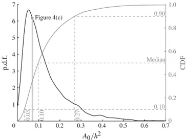
0.2 0.4 0.6 0.8 0.10 Median 0.90 0.03 0.10 0.27 1 2 3 4 5 6 p.d.f. 7 Figure 4(c) 0.1 0.2 0.3 0.4 0.5 0.6 0 0.70 1.0 CDF

FIGURE 6. Probability density function (p.d.f.) and cumulative density function (CDF) for A0. The p.d.f. has a long right-tail indicating a small number of instances for which the area of

reverse flow is large.

function f ·Φ(f ) of the streamwise position of the centroid of A0(t). Instances of no separation are represented in the frequency analysis by a centroid position of x_{/h = 0. A peak is observed at St = 0.09, which is equivalent to a frequency of} approximately 30 Hz. Therefore, the data set contains over 100 full representations of the dominant frequency, which is a sufficient number on which to base a statistical analysis. Although certain aspects of the results may not be completely statistically converged, the dominant mechanisms can still be identified with the current data.

Figure 6 shows the probability density function (p.d.f.) and cumulative distribution function (CDF) of A0 for the present data. The p.d.f. is positively skewed with the median at A0/h2= 0.1. The maximum instance of reverse flow has an area equivalent to 0.7h2 _{and therefore represents a massive separation event in the step corner. The} distribution right-tail is highly elongated and the CDF shows that only 10 % of data has reverse flow in excess of A0/h2= 0.27. Conversely, the p.d.f. also shows that some PIV fields show no reverse flow at all. While this may be accurate, it must be taken in context of the experimental limitations of PIV. Surface glare makes it difficult to calculate vectors close to a wall and the wall-normal location closest to the wall in the present study has a coordinate of y_{/h = 0.04 (or y = 1.2 mm). It is therefore possible} that reverse flow occurred outside the spatial domain captured in this study. The same is true for the vertical wall of the step for which the most upstream streamwise coordinate of a datapoint is x_{/h = −0.02 (or x = −0.6 mm).}

3.1. Representative separation point using conditional averaging

The value of A0 for the example PIV velocity field shown in figure 4(c) is labelled in figure 6. It can be seen that the example image has a reverse flow area A0 close to the peak of the p.d.f. and is therefore a commonly occurring value. To learn more about the structure of separation for an A0 of this magnitude, it would be useful to inspect the streamline pattern. However, little can be inferred from the streamlines of an instantaneous turbulent velocity field. So instead we inspect the streamlines of a conditionally averaged velocity field, conditioned over a small range of A0. A suitable

, on

30 May 2017 at 13:57:45

.

(10)

range for the example velocity field of figure4is highlighted in figure6as the vertical band of light grey between the two scalar limits A0/h2= [a, b] = [0.07, 0.075].

Figure 7(a) shows the streamlines computed from conditionally averaging the streamwise and wall-normal velocity components over the same limits (0.07 < A0/h2< 0.075). This bin contains the example velocity field of figure 4. The separation region is visible clearly, with a large separation bubble. There is no reattachment point on the step face, only a stagnation point outside of the separated flow. This is the ‘open’ type separation as described by the studies of St¨uer et al. (1999), Wilhelm et al. (2003) and Lanzerstorfer & Kuhlmann (2012). The open separation entrains fluid incident on the step face by rolling it into the vortex core.

The average streamlines of figure 7(a) are sufficiently coherent that a direct approximation of the point of separation is possible. However, identifying the exact separation point in turbulent flow is not trivial. The separation point is unsteady with regions of local three-dimensionality. This difficulty is addressed in the reviews by Simpson (1989, 1996), which explain that only in steady two-dimensional flow does a turbulent separation point necessarily coincide with the classic definition: the point at which the average wall shear stress hτwalli is zero. Instead, Simpson (1989) proposed that for turbulent flow a more reliable measure is the fraction of time any spatial location experiences downstream flow. This fraction is denoted γ and the location at which hγ i = 0.5 is named transitory detachment. In practice, the locations at which hγ i = 0.5 and hτwalli = 0 are often found to coincide (Na & Moin 1998). For the data in figure7(a) the two estimates are in close agreement, with a value of xsep/h ≈ −0.5.

Figures 7(b)–(d) show conditionally averaged streamlines and the separation estimation for three other bins of A0, each showing very different separation characteristics. Figure 7(b) shows a bounded separation bubble in the step corner, with a reattachment point on the step face. The separation is now ‘closed’ and there is no longer direct in-plane entrainment of the boundary layer into the separation. Despite no longer entraining fluid from the oncoming boundary layer, the closed separation is still subject to out-of-plane (spanwise) mass fluxes along the step corner which, as demonstrated by St¨uer et al. (1999), is a crucial mechanism by which the separation changes shape. Figure7(b) is the lowest range of A0 exhibiting a closed separation and it occurs close to the median value of A0. Therefore, approximately half of all flow instances have an open separation.

In figure 7(c) the separatrix now extends up and over the step, meaning that mass from within the separation region is leaked over the top of the step. There remains a reattachment point on the step face, but it is now contained wholly within the separation region. The ejection of separated flow over the step corner was shown in the experimental work of St¨uer et al. (1999) and the simulations by Wilhelm et al. (2003) and Lanzerstorfer & Kuhlmann (2012). These studies all demonstrated that the corner vortex rolls up, travels spanwise along the corner until it eventually spills into the downstream flow. These results were measured and verified in a laminar flow, but figure 7(c) suggests that a qualitative read across to turbulent flow holds. This observation is reinforced by the streamlines in figure 7(d) which shows a massive separation event where the whole vortex structure of the upstream separation is evacuated over the step, an event which St¨uer et al. (1999) referred to as a streak.

Figure7(e) shows the distribution of separation points for a sequence of consecutive bins covering the whole range of A0, calculated using both the hτwalli and hγ i methods. The separation points of the four streamline patterns of figures 7(a)–(d) are labelled. The general trend of the data in figure 7(e) is that the separation point xsep moves upstream as A0 increases, then remains at approximately x/h = −1.2 for

, on

30 May 2017 at 13:57:45

.

(11)

Median 0.2 0.4 0.6 0.8 1.0 1.2 1.4 1.6 (a) –2.0 –1.5 –1.0 –0.5 0.2 0.4 0.6 0.8 1.0 1.2 1.4 1.6 (b) –2.0 –1.5 –1.0 –0.5 0.2 0.4 0.6 0.8 1.0 1.2 1.4 1.6 (c) (e) –2.0 –1.5 –1.0 –0.5 0.2 0.4 0.6 0.8 1.0 1.2 1.4 1.6 (d) –2.0 –1.5 –1.0 –0.5 –1.2 –1.0 –0.8 –0.6 –0.4 –0.2 0 0.1 0.2 0.3 0.4 0.5 0.6 0 0.7 (a) (b) (c) (d)

FIGURE7. Streamlines and point of separation for conditional averages of the flow based on A0. As the streamwise position of separation in (e) moves upstream, different characteristics

of the conditionally-averaged separation are observed: (a) streamlines for bin 0.070 < A0/h2< 0.075, containing 1034 vector fields; (b) streamlines for bin 0.115 < A0/h2< 0.120,

containing 693 vector fields; (c) streamlines for bin 0_{.180 < A}0/h2< 0.185, containing 306

vector fields; (d) streamlines for bin 0_{.500 < A}0/h2< 0.520, containing 67 vector fields;

(e) summary of separation point estimates for all A0bins.

, on

30 May 2017 at 13:57:45

.

(12)

all A0/h2> 0.4. At very low values of A0, the value of xsep could not be calculated because the data contained little or no reverse flow, possibly due to the experimental limitation previously mentioned.

Overall, the two separation identification methods, τwall and γ , are in good agreement and show upstream movement of the separation point with increases in reverse flow. Common to both methods is the low scatter of xsep for averages of reverse flow less than the median. This suggests that for instances of open separation as depicted in figure7(a) xsep moves upstream in a predictable manner as A0 increases. However, once the separation grows large enough to form a reattachment on the step face, the scatter in xsep increases. This can be attributed to the y-fluctuations of the reattachment point on the step face and the corresponding occasional transfer of mass from inside the separation region to over the step face. Nevertheless, there is a continued upstream movement of xsep until approximately A0/h2= 0.4. For averages of reverse flow larger than this, there is little change in the separation position. This implies that any further increase in the volume of fluid in the separation region is balanced by that expelled over the top of the step.

3.2. Spatial extent of reverse flow

The relation between the magnitude and spatial distribution of the reverse flow can be further investigated by examining the relationship between A0 and the spatial extremity of the reverse flow. The most upstream location of U_{(x, y, t) < 0 is denoted here as} x0(t)/h and the highest wall-normal extent of U(x, y, t) < 0 is denoted here as y0(t)/h. These quantities can be regarded as the minimum spatial extent of the separation region at any time, since, in the present study, reverse flow only occurs within the bounds of the separated flow. The relation between x0 and y0 relative to A0 reveal the nature of changes in size of the reverse flow with time.

Figure 8(a) and (b) show the temporal cross-correlations Rx0,A0 and Ry0,A0, respectively. Both correlation peaks are close to 0_{.7. This demonstrates a strong} linear dependence between the extent of reverse flow and the total area of reverse flow. In addition, the peaks of figure 8(a) and (b) are both centred on zero, meaning an increase in A0 results in a simultaneous increase in extent of reverse flow in both streamwise and wall-normal directions.

Figure 8(c) and (d) show the joint p.d.f. of A0 with the same variable pairings, x0 and y0, respectively. Each joint p.d.f. has been normalized so the area enclosed by the contours is unity. Also shown on these figures is the conditional averages of x0 and y0 for a sequence of consecutive bins conditioned on the value of A0 (the conditional average is computed using the procedure outlined in the previous section). Figure 8(c) and (d) show that the reverse flow remains bounded within a small spatial region the majority of the time, with departures from this region infrequent but large. This is consistent with the findings in §3.1 where for over half of all flow instances the separation region was a compact open vortex that remained close to the step face. It is clear the linear relation captured by figure 8(a) and (b) holds reasonably well for small A0, but the large infrequent departures are nonlinear and are likely caused by the separation region spilling over the step corner into the downstream flow, as identified in §3.1.

4. Influence of the upstream flow on separation

A series of experiments (see Hillier & Cherry 1981; Kiya & Sasaki 1983; Saathoff & Melbourne 1997) demonstrated that the separation region from the leading edge of

, on

30 May 2017 at 13:57:45

.

(13)

0 –0.5 0.5 (a) (c) –20 –10 0 10 20 0 (b) (d ) –20 –10 0 10 20 (0, –0.68) –0.5 0.5 (0, 0.67) –1.0 –0.5 0.1 0.2 0.3 0 –1.5 0 0.2 0.4 0.6 0.8 1.0 0.1 0.2 0.3 0 0 2 4 8 12 16 20 24 28 0.4 0 1 2 4 6 8 10 12 14 0.4

FIGURE 8. Comparison of streamwise (x0) and wall-normal (y0) extent of separation region

with area of reverse flow (A0). Temporal cross-correlation of A0 with (a) x0 and (b) y0.

(c) Joint p.d.f. of A0 and x0 with conditional averages hx0| a < A0/h2< bi and (d) Joint

p.d.f. of A0 and y0 with conditional averages hy0| a < A0/h2< bi. Greyscale is probability

density, normalized so total probability is unity.

a bluff body is strongly modulated by oncoming turbulent disturbances, which cause a roll up of the vortices in the shear layer and lead to increased turbulent intensity within the separated region. It is a reasonable assumption that similar mechanical processes are present in a forward-facing step flow. Indeed the laminar stability analyses of Wilhelm et al. (2003) and Lanzerstorfer & Kuhlmann (2012) showed that the upstream perturbations propagate downstream and cause temporal instabilities such as the vortex roll up.

To investigate whether such dependencies exist in the turbulent case, we wish to inspect the set of images comprising the conditional average (3.4) at different points in time. For any time offset_{τ, the conditional average of the time-shifted set of images is}

hU (t + τ)it∈T[a,b]. (4.1)

The condition imposed for these averages is identical to that in the previous section, i.e. the total area of reverse flow within a certain range. In this section, the primary interest is the properties of the flow where _{τ < 0 for bins of high and low A}0. This will show, on average, the properties of the boundary layer leading up to the instances of extreme separation size. We begin by inspecting the conditional averages of high A0 contained in the bin [a, b] = [0.27, 0.7], which (with reference to figure 6) represents the largest 10 % of all A0.

Figure9 shows the field of velocity perturbations u0_{for a sequence of 10 conditional} averages of the bin [a, b] = [0.27, 0.7] at time instances between τU∞/h = −18 to 0. Dark shading indicates a velocity deficit with respect to the mean flow. For τU∞/h = −18 to −10, the sequence shows a large region of low-velocity fluid moving downstream towards the step. The front of the region is inclined to the

, on

30 May 2017 at 13:57:45

.

(14)

1.0 0.5 1.5 –5 –4 –3 –2 –1 0 –0.02 –0.04 –0.06 –0.08 15°

FIGURE9. Conditional averages hu0(t +τ)i over the maximum 10 % of A0(t)/h2, time-shifted

by_τU_∞_{/h = −18 to 0. A low-velocity region is seen moving downstream prior to the large} separation event. The inclination of the low-velocity region is approximately 15◦_.

wall, as is characteristic for coherent structures convecting in the outer boundary layer (Robinson 1991). The angle of inclination of the low-velocity region when far from the step is approximately 15◦_{. This is consistent with the behaviour of the} low-velocity region generated at the centre of a system of interacting hairpin vortices (see Head & Bandyopadhyay 1981, Zhou et al. 1999, Adrian, Meinhart & Tomkins

2000, Christensen & Adrian 2001 and Ganapathisubramani et al. 2005 among various others). Such systems are the result of ejections of low-velocity fluid from the near-wall region which coalesce and can penetrate the full thickness of the boundary layer. Adrian et al. (2000) showed that the mean inclination of the upstream side of these regions, in a zero-pressure gradient flow, is typically 12◦_{, but can range from anywhere} between 3 and 30◦_.

As the flow approaches the step and the pressure gradient can no longer be considered negligible, figure 9 shows that the angle of the low-velocity front increases because the flow rises to pass the step face (due to the adverse pressure gradient imposed by the presence of the step). At _τU_∞_{/h = −6, the low-velocity region} reaches the step face and surrounds the separation region. The conditional averages

, on

30 May 2017 at 13:57:45

.

(15)

atτU∞/h = −4 to 0 then show a sudden and localized emergence of very low-velocity fluid from within the separation region. This dramatic velocity deficit is due to the spanwise movement of separated flow entering the PIV plane at the step corner as observed by St¨uer et al. (1999), Wilhelm et al. (2003) and Lanzerstorfer & Kuhlmann (2012) and described in §3.1.

The sequence of events in figure 9 shows that occurrences of the separation region expanding over the step face are, on average, preceded by a region of low-velocity fluid convecting over the step from upstream. The momentum deficit at the step face caused by the low-velocity region means fluid is then drawn from adjacent spanwise locations into the separation. The separated region (in the plane of the initial momentum deficit) then swells and eventually expands over the step face into the downstream flow. This suggests that the transverse movement of fluid along the step face is dominant in determining the size of the separation, but this is influenced by, and perhaps modulated by, velocity perturbations with their origins upstream.

This process can be further described by inspecting the perturbations in displacement thickness, δ∗0_{, of the flow under the same conditional average criteria} for the maximum 10 % of A0, that is

hδ∗0_{(x, t + τ)i}

t∈T[0.29,0.7], (4.2)

whereδ∗0_{= δ}∗_{− δ, and δ is the mean displacement thickness.}

Figure 10_{(a) shows contours of constant hδ}∗0_{i over varying streamwise location} x and time-shift _{τ. A high δ}∗0 _{represents a higher than average velocity deficit of} the boundary layer relative to the free stream and vice versa. Lines of constant convection velocity relative to the free stream are shown bottom left and the position of hxsep(t + τ)i is shown by a line on the right. Figure 10(b) and (c) are taken directly from the data in figure 10(a) and show line transects of constant x and constant _τ, respectively.

The diagonal striations in figure 10(a) represent the convection of disturbances downstream with time. The angle of the striae indicates the local convection velocity. The notable feature is the dark ‘ridge’ shown starting at τU∞/h = −15. It represents a region of velocity deficit moving downstream at close to U_∞, gradually decelerating in the vicinity of the step, then leading into the region of very high δ∗0 _{at x}_{/h > −1. The} point where this reaches the separated region coincides with the sudden increase in xsep. This same effect is also shown by the successive maxima of figure 10(b) leading to a large velocity deficit at x_{/h = −1. Figure} 10(c) accentuates how localized and sudden the rise in velocity deficit is, which confirms the dominance of the effect of streamwise flow along the step face on the size and dynamics of the separation region.

An equivalent analysis can be made for instances of small separation. Figure 11(a) shows the contour plot for the conditional average of hδ∗0_{i for the limits [a, b] =} [0, 0.03]; a bin comprising the lowest 10 % of A0. As for the highest 10 %, the change in separation size is relatively sudden and confined, also suggesting localized three-dimensional causes. The contours of figure 11(a) show a gradual and global reduction of the velocity deficit in both x and τ prior to the incident of minimum reverse flow.

This is shown most clearly in figure 11(b) by the negative gradient of all x/h transects which, with the exception of x_{/h = −1, level off at hδ}∗0_{i = 0. Similarly, the} upstream hδ∗0_{i plateau in figure} ₁₁_{(c) steadily falls back to zero from a previous high} of 0.02. These trends show that rather than the incident of low reverse flow being caused by a specific upstream disturbance, it follows a more global restoration of the mean flow conditions after a period of large velocity deficit.

, on

30 May 2017 at 13:57:45

.

(16)

1.0 0.6 0.4 (a) (b) (c) –20 –15 –10 –5 0 5 –5 –4 –3 –2 –1 xsep 0.01 0.02 0.03 0.04 0.05 0.06 0.07 0.08 0.09 –14 –12 –10 –8 –6 –4 –2 0 0.10 –16 0 –5 –4 –3 –2 –1 0.02 0.04 0.06 0.08 0.10 0.12 0.14 0.16 0.18 0 0.20 –4 –3 –2 –1 0 –5 –10 0 –2 –4 –6 –8 –0.08 –0.06 –0.04 –0.02 0 0.02 0.04 0.06 0.08

FIGURE 10. Conditional average hδ∗0(t + τ)i/h over the maximum 10 % of A0(t)/h2.

(a) Contours of constant _δ∗0_{/h in x/h and τU}_∞_{/h. The movement of the low-velocity}

region of figure 9 is represented by the dark striation. When the region reaches the step the separation point moves upstream. Transects at constant streamwise location and constant time offset are shown in (b) and (c), respectively.

4.1. Discussion on possible upstream influences

The data presented shows that large separation events in front of the step are preceded by forward-inclined regions of low and high velocity in the outer region of the turbulent boundary layer. The existence of such energetic structures in the outer region of turbulent boundary layers is well-established (Kovasznay, Kibens & Blackwelder

1970, Blackwelder & Kovasznay 1972, Brown & Thomas 1977 and Wark & Nagib

1991 among others). They are in the form of elongated low- and high-speed regions

, on

30 May 2017 at 13:57:45

.

(17)

1.0 0.6 0.4 (a) (b) (c) –20 –15 –10 –5 0 5 –5 –4 –3 –2 –1 –4 –3 –2 –1 0 –5 –0.01 –0.02 –0.03 –0.04 0.01 0.02 0.03 0.04 0 –5 –4 –3 –2 –1 –10 –8 –6 –4 –2 0 –10 –2 –4 –6 –8 0 –0.04 –0.06 –0.08 –0.10 –0.02 0 0.02 0.04 –0.12 0.06 –0.08 –0.06 –0.04 –0.02 0 0.02 0.04 0.06 0.08

FIGURE_{11. Conditional average hδ}∗0(t + τ)i over the minimum 10 % of A0(t). (a) Contours

of constant δ∗0_{/h in x and τ. (b) Transects at constant streamwise location. (c) Transects at}

constant time offset.

that meander in the spanwise direction. An understanding of their nature and influence was developed by the studies of Adrian et al. (2000), Ganapathisubramani, Longmire & Marusic (2003), Tomkins & Adrian (2003) and Ganapathisubramani et al. (2005), who explained their presence in terms of packets of vortical structures surrounding a long core of low momentum. The streamwise length of these regions was measured to be between 2_{δ and 3δ, but this was limited by the PIV field of view and it was} suspected they extended much further. This was confirmed by the experiments of Hutchins & Marusic (2007), in which a rake of hotwires was used in conjunction with Taylor’s frozen-flow hypothesis to estimate that the structure length was in

, on

30 May 2017 at 13:57:45

.

(18)

excess of 20δ. Owing to their size as well as their energy content, these structures were termed as superstructures. Further investigation showed that superstructures existed at very high Reynolds number (Marusic & Hutchins 2008) and in supersonic boundary layer flows (Ganapathisubramani, Clemens & Dolling 2006). In the study by Ganapathisubramani, Clemens & Dolling (2007), superstructures of length up to 40_{δ were observed upstream of a ramp in a supersonic boundary layer. These} structures, comprising long regions of adjacent high and low flow speed, the same as those of a subsonic boundary layer, were shown to affect the instantaneous position of the separation and were used to explain the low-frequency unsteadiness of the shock-induced separation region. This phenomenon was also observed in an impinging shock-induced separation by Humble, Scarano & van Oudheusden (2009).

If the separation events in the present study are being influenced, modulated or caused by an interaction with these elongated structures in the upstream boundary layer, then, as in the work of Ganapathisubramani et al. (2007), it follows that both dynamic processes will exist over comparable time scales. Figure5 shows the motion of the centroid of the reverse flow region has a dominant frequency (normalized by step height) of Sth= 0.09. However, the peak of this power spectrum is relatively rounded and a dominant range of frequencies can be identified as Sth = 0.03–0.15. If, for comparison with other studies, the Strouhal number is expressed in terms of the boundary layer thickness _{δ = 0.044 m and a representative convection velocity} of Uc= 0.8U∞= 8 m s−1, this range becomes Stδ = 0.042–0.2. This equates to a boundary layer time scale of 1/Stδ= 5–24.

Now, figures 10(a) and 11(a) indicate that the low-velocity perturbations are responsible only for the growth of the separation region, not the subsequent decay. Therefore, the direct influence of the convecting low-velocity region is only over half a bubble ‘cycle’, i.e. it is present for half the time scale. This means the streamwise length of a low-velocity region that corresponds to the time scales of the growth of the separation bubble lies in the approximate range 2δ to 12δ. This range, inclusive of the simplifications and assumptions stated, is consistent with the length of structures identified in the aforementioned literature. Indeed, the meandering nature of the superstructures means that a two-dimensional field, as in the present study, will seldom capture the full streamwise extent of the low-velocity region. This meandering nature may also go some way to explaining the low-frequency spanwise motions of the separation streaks observed in the experiments by St¨uer et al. (1999).

5. Conclusions

The separation region upstream of a forward-facing step is known to have complex dynamic interactions with the upstream, downstream and spanwise flow along the step. These interactions have been investigated for laminar flows, but this is the first known experimental investigation of the dynamics of the upstream separation in a fully turbulent boundary layer. It has been shown that similar physical processes to those observed in laminar flows, such as vortex roll up and spanwise flow leading to the creation of streaks over the top of the step, are present.

Conditional averaging based on the area of reverse flow demonstrates that the turbulent separation region exhibits both open and closed forms. The separation region is of open form for approximately 50 % of the time. Closed-form bubbles have a reattachment point on the step face, which occasionally rises over the step corner leading to a growth of the separation region and the expulsion of fluid downstream. The growth of the separation bubble happens in both the wall-normal and streamwise

, on

30 May 2017 at 13:57:45

.

(19)

directions simultaneously. At large instances of reverse flow, the upstream movement of the separation point is limited by the transfer of mass over the step corner.

It has been shown that the large separation events are preceded by the presence of low-velocity regions that originate in the upstream boundary layer and then convect over the step. Instances of low reverse flow are preceded by a general increase in the global flow velocity over the domain. The suddenness of the separation bubble growth and decay suggests the dominant mechanism determining the separation characteristics is the transverse flow along the step corner, which in turn is modulated by the structures in the upstream flow.

The length, position and inclination of these low-velocity regions is consistent with that in the published literature on turbulent boundary layers. The time scales associated with the build-up of a large separation region is consistent with the passage of these elongated low-velocity regions. Detection of these regions could potentially be used as the basis for a control scheme to stabilize the upstream separation. However, a suitable control objective, and the characteristics of the actuation required to achieve it, remain topics for further study.

Acknowledgements

Financial support for this work from the EPSRC, through grant number EP/F056206/1, is greatly appreciated, as is the funding received from the European Union Seventh Framework Programme FP7/2007-2013 under the grant agreement number FP7-ICT-2009-4 248940.

We also thank the technicians and other colleagues Imperial College London who aided us in design and setup of the experiments.

R E F E R E N C E S

ADDAD, Y., LAURENCE, D., TALOTTE, C. & JACOB, M. C. 2003 Large eddy simulation of a

forward-backward facing step for acoustic source identification. Intl J. Heat Fluid Flow 24, 562–571.

ADRIAN, R. J., MEINHART, C. D. & TOMKINS, C. D. 2000 Vortex organization in the outer region

of the turbulent boundary layer. J. Fluid Mech. 422, 1–54.

ADRIAN, R. J. & MOIN, P. 1988 Stochastic estimation of organized turbulent structure:

homogeneous shear flow. J. Fluid Mech. 190, 531–559.

ARIE, M., KIYA, M., TAMURA, H., KOSUGI, M. & TAKAOKA, K. 1975 Flow over rectangular cylinders immersed in a turbulent boundary layer. Bull. Japan Soc. Mech. Eng. 18 (125), 1260–1268.

BLACKWELDER, R. F. & KOVASZNAY, L. S. G. 1972 Time scales and correlations in a turbulent boundary layer. Phys. Fluids 15, 1545–1554.

BROWN, G. R. & THOMAS, A. S. W. 1977 Large structure in a turbulent boundary layer. Phys. Fluids20, S243–S251.

CAMUSSI, R., FELLI, M., PEREIRA, F., ALOISIO, G. & DI MARCO, A. 2008 Statistical properties

of wall pressure fluctuations over a forward-facing step. Phys. Fluids 20 (075113).

CHRISTENSEN, K. T. & ADRIAN, R. J. 2001 Statistical evidence of hairpin vortex packets in wall

turbulence. J. Fluid Mech. 431, 433–443.

CORINO, E. R. & BRODKEY, R. S. 1969 A visual investigation of the wall region in turbulent flow.

J. Fluid Mech.37 (1), 1–30.

EFIMSTOV, B. M., GOLUBEV, A. YU., RIZZI, S. A., ANDERSSON, A. O. & ANDRIANOV, E. V.

2002 Influence of small steps on wall pressure fluctuation spectra measured on TU-144LL flying laboratory. AIAA 2002–2605.

GANAPATHISUBRAMANI, B., CLEMENS, N. T. & DOLLING, D. S. 2006 Large-scale motions in a supersonic turbulent boundary layer. J. Fluid Mech. 556, 271–282.

, on

30 May 2017 at 13:57:45

.

(20)

GANAPATHISUBRAMANI, B., CLEMENS, N. T. & DOLLING, D. S. 2007 Effects of upstream

boundary layer on the unsteadiness of shock-induced separation. J. Fluid Mech. 585, 369–394.

GANAPATHISUBRAMANI, B., HUTCHINS, N., HAMBLETON, W. T., LONGMIRE, E. K. & MARUSIC, I. 2005 Investigation of large-scale coherence in a turbulent boundary layer using two-point correlations. J. Fluid Mech. 542, 57–80.

GANAPATHISUBRAMANI, B., LONGMIRE, E. K. & MARUSIC, I. 2003 Characteristics of vortex packets in turbulent boundary layers. J. Fluid Mech. 478, 35–46.

HATTORI, H. & NAGANO, Y. 2010 Investigation of turbulent boundary layer over forward-facing step via direct numerical simulation. Intl J. Heat Fluid Flow 31 (3), 284–294.

HEAD, M. R. & BANDYOPADHYAY, P. 1981 New aspects of turbulent boundary-layer structure.

J. Fluid Mech. 107, 297–338.

HILLIER, R. & CHERRY, N. J. 1981 The effects of stream turbulence on separation bubbles. J. Wind Engng Ind. Aerodyn.8, 49–58.

HUMBLE, R. A., SCARANO, F. &VAN OUDHEUSDEN, B. W. 2009 Unsteady aspects of an incident

shock wave/turbulent boundary layer interaction. J. Fluid Mech. 635, 47–74.

HUTCHINS, N. & MARUSIC, I. 2007 Evidence of very long meandering features in the logarithmic region of turbulent boundary layers. J. Fluid Mech. 579, 1–28.

JI, M. & WANG, M. 2010 Sound generation by turbulent boundary-layer flow over small steps.

J. Fluid Mech. 654, 161–193.

KIYA, M. & SASAKI, K. 1983 Free-stream turbulence effects on a separation bubble. J. Wind Engng Ind. Aerodyn.14, 375–386.

KOVASZNAY, L. S. G., KIBENS, V. & BLACKWELDER, R. F. 1970 Large-scale motion in the intermittent region of a turbulent boundary layer. J. Fluid Mech. 41, 283–325.

LANZERSTORFER, D. & KUHLMANN, H. C. 2012 Three-dimensional instability of the flow over a

forward-facing step. J. Fluid Mech. 695, 390–404.

LARGEAU, J. F. & MORINIERE, V. 2007 Wall pressure fluctuations and topology in separated flows over a forward-facing step. Exp. Fluids 42, 21–40.

LECLERCQ, D. J. J., JACOB, M. C., LOUISOT, A. & TALOTTE, C. 2001 Forward-backward facing

step pair: Aerodynamic flow, wall pressure and acoustic characterisation. In Proceedings of the Seventh AIAA/CEAS Aeroacoustics Conference, vol. AIAA-2001-2249. Maastricht.

MARINO, L. & LUCHINI, P. 2009 Adjoint analysis of the flow over a forward-facing step. Theor. Comput. Fluid Dyn.23 (1), 37–54.

MARTINUZZI, R. & TROPEA, C. 1993 The flow around surface-mounted, prismatic obstacles placed

in a fully developed channel flow. J. Fluid Engng 115, 85–92.

MARUSIC, I. & HUTCHINS, N. 2008 Study of the log-layer structure in wall turbulence over a very large range of Reynolds number. Flow Turbulence Combust. 81, 115–130.

MOHSEN, A. M. 1967 Experimental investigation of the wall pressure fluctuations in subsonic

separated flows. Tech. Rep. D6-17094. The Boeing Company.

MOSS, W. D. & BAKER, S. 1980 Re-circulating flows associated with two-dimensional steps. Aeronaut. Q.31, 151–172.

NA, Y. & MOIN, P. 1998 Direct numerical simulation of a separated turbulent boundary layer. J. Fluid Mech. 374, 379–405.

ROBINSON, S. K. 1991 Coherent motions in the turbulent boundary layer. Annu. Rev. Fluid Mech.

23, 601–639.

SAATHOFF, P. J. & MELBOURNE, W. H. 1997 Effects of free stream turbulence on surface pressure fluctuations in a separation bubble. J. Fluid Mech. 337, 1–24.

SHERRY, M., LO JACONO, D. & SHERIDAN, J. 2010 An experimental investigation of the

recirculation zone formed downstream of a forward facing step. J. Wind Engng Ind. Aerodyn. 98, 888–894.

SIMPSON, R. L. 1989 Turbulent boundary-layer separation. Annu. Rev. Fluid Mech. 21, 205–232. SIMPSON, R. L. 1996 Aspects of turbulent boundary-layer separation. Prog. Aerosp. Sci. 32 (5),

457–521.

STUER¨ , H., GYR, A. & KINZELBACH, W. 1999 Laminar separation on a forward facing step.

Eur. J. Mech. (B/Fluids) 18, 675–692.

, on

30 May 2017 at 13:57:45

.

(21)

TOMKINS, C. D. & ADRIAN, R. J. 2003 Spanwise structure and scale growth in turbulent boundary

layers. J. Fluid Mech. 490, 37–74.

WARK, C. E. & NAGIB, H. M. 1991 Experimental investigation of coherent structures in turbulent

boundary layers. J. Fluid Mech. 230, 183–208.

WILHELM, D., HARTEL, C. & KLEISER, L. 2003 Computational analysis of the two-dimensional–three-dimensional transition in forward-facing step flow. J. Fluid Mech. 489, 1–27.

WILLMARTH, W. W. & LU, S. S. 1972 Structure of the Reynolds stress near the wall. J. Fluid Mech.55, 65–92.

ZHOU, J., ADRIAN, R. J., BALACHANDAR, S. & KENDALL, T. M. 1999 Mechanisms for generating coherent packets of hairpin vortices in channel flow. J. Fluid Mech. 387, 353–396.

, on

30 May 2017 at 13:57:45

.