A Dynamic Duopoly Investment Game without Commitment under Uncertain Market Expansion

Texte intégral

(1)2011s-65. A Dynamic Duopoly Investment Game without Commitment under Uncertain Market Expansion Marcel Boyer, Pierre Lasserre, Michel Moreaux. Série Scientifique Scientific Series. Montréal Octobre 2011. © 2011 Marcel Boyer, Pierre Lasserre, Michel Moreaux. Tous droits réservés. All rights reserved. Reproduction partielle permise avec citation du document source, incluant la notice ©. Short sections may be quoted without explicit permission, if full credit, including © notice, is given to the source..

(2) CIRANO Le CIRANO est un organisme sans but lucratif constitué en vertu de la Loi des compagnies du Québec. Le financement de son infrastructure et de ses activités de recherche provient des cotisations de ses organisations-membres, d’une subvention d’infrastructure du Ministère du Développement économique et régional et de la Recherche, de même que des subventions et mandats obtenus par ses équipes de recherche. CIRANO is a private non-profit organization incorporated under the Québec Companies Act. Its infrastructure and research activities are funded through fees paid by member organizations, an infrastructure grant from the Ministère du Développement économique et régional et de la Recherche, and grants and research mandates obtained by its research teams. Les partenaires du CIRANO Partenaire majeur Ministère du Développement économique, de l’Innovation et de l’Exportation Partenaires corporatifs Autorité des marchés financiers Banque de développement du Canada Banque du Canada Banque Laurentienne du Canada Banque Nationale du Canada Banque Royale du Canada Banque Scotia Bell Canada BMO Groupe financier Caisse de dépôt et placement du Québec CSST Fédération des caisses Desjardins du Québec Financière Sun Life, Québec Gaz Métro Hydro-Québec Industrie Canada Investissements PSP Ministère des Finances du Québec Power Corporation du Canada Rio Tinto Alcan State Street Global Advisors Transat A.T. Ville de Montréal Partenaires universitaires École Polytechnique de Montréal HEC Montréal McGill University Université Concordia Université de Montréal Université de Sherbrooke Université du Québec Université du Québec à Montréal Université Laval Le CIRANO collabore avec de nombreux centres et chaires de recherche universitaires dont on peut consulter la liste sur son site web. Les cahiers de la série scientifique (CS) visent à rendre accessibles des résultats de recherche effectuée au CIRANO afin de susciter échanges et commentaires. Ces cahiers sont écrits dans le style des publications scientifiques. Les idées et les opinions émises sont sous l’unique responsabilité des auteurs et ne représentent pas nécessairement les positions du CIRANO ou de ses partenaires. This paper presents research carried out at CIRANO and aims at encouraging discussion and comment. The observations and viewpoints expressed are the sole responsibility of the authors. They do not necessarily represent positions of CIRANO or its partners.. ISSN 1198-8177. Partenaire financier.

(3) A Dynamic Duopoly Investment Game without Commitment under Uncertain Market Expansion* Marcel Boyer†, Pierre Lasserre ‡, Michel Moreaux§. Résumé / Abstract We model capacity-building investments in a homogeneous product duopoly facing uncertain demand growth. Capacity building is achieved through the addition of production units that are durable and lumpy and whose cost is irreversible. While building their capacity over time, firms compete à la Cournot in the product market given their installed capacity. There is no exogenous order of moves, no commitment regarding future decisions, and no finite horizon. We investigate Markov Perfect Equilibrium (MPE) paths of the investment game, which may include episodes during which firms invest at different times, a preemption pattern, and episodes in which firms invest simultaneously, a tacit collusion pattern. These episodes may alternate and are typically several. When firms have yet to invest in capacity, the sole pattern that is MPE-compatible is a preemption episode: firms invest at different times but have equal value. The first such investment may occur earlier and therefore be riskier than socially optimal. When both firms hold capacity, tacit collusion episodes may be MPEcompatible: firms invest simultaneously at a postponed time (hence holding back production in the meantime), thereby generating an investment wave in the industry. Such investment episodes are more likely with higher demand volatility, faster market growth, and lower cost of capital (discount rate). Mots clés/Keywords : Real Options; Dynamic Duopoly; Lumpy Investments; Preemption; Investment Waves; Tacit Collusion. Codes JEL : C73, D43, D92, L13.. *. We are grateful to Thomas Mariotti, Bruno Versaevel, participants in conferences at Georgetown University and École des Dirigeants et Créateurs d’entreprises (EDC), in the Conference in honor of Claude Henry (Paris), as well as in seminars at USC, Penn State, UBC and UZH for their comments. Moreover, comments from two anonymous referees as well as the Editor were quite helpful in improving the paper. Financial support from CIRANO, CIREQ, SHRCC (Canada) and INRA (France) is gratefully acknowledged. † Bell Canada Emeritus Professor of Industrial Economics, Université de Montréal, marcel.boyer@umontreal.ca. ‡ Department of Economics, Université du Québec à Montréal, lasserre.pierre@uqam.ca. § Toulouse School of Economics at Université de Toulouse 1 Capitole, mmichel@cict.fr..

(4) 1. Introduction. Investment games played by competing firms in oligopolistic markets typically share the following stylized characteristics: (i) the development of the market is uncertain, but firms have similar knowledge of the underlying random process generating the market development; (ii) firms’ production capacities are built over time through additional units of significant size; (iii) investments in real assets are substantially irreversible; (iv) firms compete in the product market, given their installed production capacities, while they can at the same time develop those capacities; (v) any firm may invest at any time as the market develops and as its competitors build their own capacity; (vi) at the industry level, new investments sometimes come in waves with firms building new plants simultaneously and sometimes in sequences with firms investing at different dates; (vii) as the market matures, absent drastic innovations, capacity building eventually comes to an end determined by the potential market size, with capacities remaining essentially the same for an indefinite time. We develop a duopoly model with features (i) to (v) above, which generates results (vi) and (vii) among others. More specifically, we consider a homogeneous product duopoly industry whose market demand is growing in a stochastic way. Firms compete continuously ` a la Cournot on the product market and they build up their capacity over time through the acquisition of lumpy units of capacity. There is no assumed or forced order of moves in capacity building, and no commitment on future investments or strategies. Rather, firms invest at chosen market development levels as they hold investment options to be exercised strategically at freely chosen dates. We characterize the value of the investment options to be exercised at the chosen timings and the value of the firms holding them. Investments are assumed irreversible and consist of indivisible capacity units that do not depreciate. Hence, capacity can only increase in discrete jumps. Market development is exogenous, stochastic, continuous, and its current level is observed by the duopolists. A state of the game is characterized by a triplet composed of the current demand level and each duopolist’s installed capacity. In any given state, a firm may decide to invest or not in one or more additional units of capacity; hence, either both firms invest in one or more capacity units, only one firm does, or neither firm does. The timing of each investment is thus linked to the stochastic state of market development, thus is itself stochastic. The present investment game is a dynamic game with no exogenously specified end. However it is not an. 1.

(5) infinitely repeated game as the continuation game is defined according to three state variables namely firms capacities and market size that are changing over time. We characterize the Markov Perfect Equilibria (MPE) of this investment game. A MPE investment path takes the form of a sequence of investment decisions by each firm as the market evolves, while firms continuously compete day to day ` a la Cournot on the product market given their installed capacity and the attained level of demand. Fudenberg and Tirole (1983, 1985) studied investment games involving a single investment by each player and found that two types of MPE may exist. One involves simultaneous or joint investment, called tacit-collusion or under-investment equilibrium because the joint investment is postponed, meaning that the firms tacitly restrict their joint production capacity, thereby lessening the day to day Cournot competition. A second type of MPE has investments occurring at different dates and was called a diffusion or preemption MPE because they emerge from early move strategies aiming at preventing the other player from investing first. In a preemption MPE, industry capacity is larger, potential rents are dissipated, and firms obtain identical payoffs despite the asymmetry in the timing of their investments. We consider an investment game involving multiple investments and admitting one or several investment paths as equilibria. In the investment game we develop and analyse in the present paper, MPE investment paths will typically be composed of different episodes, each one starting from a state characterized by the current market development and the firms’ installed capacities resulting from past decisions. Two types of episodes may appear along any given MPE investment path: episodes during which firms invest at different times, in a preemption or intense competition mode, and episodes during which firms invest simultaneously, in a tacit collusion mode. When an episode along a MPE investment path has one firm investing earlier than the other, we say by analogy with the Fudenberg-Tirole’s single-investment game that there is “preemption” during that episode, no matter what the sequence of previous or subsequent investments may be: rents are dissipated, and firms have identical incremental value. The first investment occurs precisely at the time when the market development level leaves the other firm indifferent between preempting or investing later: hence, no firm gains by moving first. When an episode along a MPE investment path has both firms investing simultaneously, we say that there is “tacit collusion” during that episode. Indeed, such simultaneous investment takes place at a higher market development level, hence later, than the levels at which firms would invest if they were to invest at different times. Industry supply is then lower during the relevant market development interval than it would be otherwise, thereby generating tacit collusion rents for the firms: capacity building is postponed, production is lower, and prices and profits are increased relative to the. 2.

(6) levels that would prevail otherwise, that is, over the same market development interval if the firms were to invest at different times in a preemption episode. We characterize the factors and conditions for which along a given MPE investment path one may encounter both preemption episodes and tacit-collusion ones.1 Our model is able to address the following questions at some level of generality: What is the link between the level of market or industry development and the intensity of competition? Do simultaneous investments or investment waves signal intense competition or tacit collusion? Can investments occur earlier than in perfect competition or in a social optimum? What is the role and effect of demand volatility, market growth rate, and cost of capital on the intensity of competition? More precisely, our main results are as follows. If firms start from a symmetric position of zero capacity when the level of market development is low, the first MPE-compatible investment episode2 is necessarily a preemption episode, with only one active firm although both firms have necessarily the same value. Eventually the investment game will come to an end either with both firms having enough capacity to produce and sell the unconstrained Cournot quantity, if there is no tacit collusion at the end of the game, or both firms forever maintaining their capacities at a lower level, if the game ends with a tacit-collusion episode. Between the initial state of zero capacities with a low market development and the end of the game, two types of investment episodes may appear along any MPE path of the investment game. Starting in any state (market development level, installed capacities) in which further investment is profitable in the future for both firms, there exists a MPE-compatible preemption episode during which firms invest at different times. In some states, which we characterize, there exists also MPE-compatible tacit collusion episodes during which both firms invest at the same time. In MPE-compatible preemption episodes, incremental rents are equalized and partly dissipated. In MPE-compatible tacit collusion episodes, firms exercise market power by postponing their respective next investment until market development reaches a threshold that exceeds the level at which either firm would have invested in a preemption episode. Firms then invest simultaneously, thereby generating an investment wave in the industry. MPE-compatible tacit collusion episodes are typically several in a given state, which are all Pareto-superior from the firms’ viewpoint to the MPE-compatible preemption episode in that given state. Furthermore, the market development trigger level at which the joint investment would maximize combined profits is MPE-compatible only if firms are of equal 1 While there is a large literature on tacit collusion in infinitely repeated games, dynamic investment games are much less well understood. For example, it is well known that collusive equilibria exist in infinitely repeated games provided firms are sufficiently patient, that is, the discount factor is sufficiently large as shoiwn for instance in Dutta (1995a, 1995b). However, no such result exists in general for non repeated games. 2 We use the terminology “MPE-compatible” to refer to an investment episode that is part of a MPE investment path.. 3.

(7) size. Hence, when firms differ in size, tacit collusion falls short of maximizing combined profits. Nevertheless, an investment wave indicates that tacit collusion has occurred and has resulted in a successful exercise of market power.3 We show that higher market volatility, faster expected market growth, as well as lower cost of capital enlarge the set of conditions under which MPE-compatible tacit collusion episodes exist. However, no such MPEcompatible tacit collusion episode exists in the early stages of market development, that is, when at least one firm holds no capacity. Even though the investment game has no finite horizon, it eventually comes to an end at some stochastic time, that is, in a state from which no further investment is undertaken by the firms. We characterize these endgame conditions. This allows us to use backward induction to characterize the MPE-compatible investment sequences. As discussed further below, this result is closely dependent on the way we model market demand growth. If along a MPE-compatible investment sequence, a point is reached where endgame conditions are close to be met while firms have different capacities, then the smaller firm will be the sole investor for a while, possibly for the remainder of the game. Thus, while firms may be of different sizes along the equilibrium path, no size advantage can be maintained forever. The related literature The present paper extends the literature on strategic investment, most notably the seminal contributions of Gilbert and Harris (1984), Fudenberg and Tirole (1985), and the more recent contribution of Besanko and Doraszelski (2004), Genc et al. (2007), and Besanko et al. (2010). These contributions brought forward the analysis of the role of investment competition in shaping the structure of a developing industry, including rent equalization and dissipation in dynamic investment games, tacit collusion conditions in such games, and the durability of a first-mover advantage. Investigating the role of investment in acquiring market dominance in a very general framework, Athey and Schmutzler (2001) came to the conclusion that, without firms’ commitment to future strategic investment plans, there is little hope to obtain definitive predictions outside specific models. In an effort to provide tractable results, modern investment games indeed were often modeled in a way that failed to exhibit some of the stylized facts mentioned above. Such models include models of technology adoption, models of entry, and numerous two-stage models where firms first make and commit to long-term decisions (stage 3 Some authors found that investment waves sometimes indicate harsh preemptive competition, as for instance in a premptive race to acquire a dominant position. Here investment waves indicate tacit collusive behavior with both firms postponing their respective acquisition of capacity units, hence holding back production and raising prices and profits in the meantime.. 4.

(8) one) before competing in short-term decisions afterwards (stage two). Although the possibility of preemption and collusion equilibria has been widely described within two-stage games,4 such games cannot account for the possible succession of intensive competition (preemption) episodes and tacitly collusive episodes along a given MPE-compatible investment path. Gilbert and Harris (1984) recognized early the role of lumpy, strategic investments in dynamic frameworks. Our endgame characterization (no size advantage can be maintained forever) is reminiscent of Gilbert and Harris (1984, Proposition 1) who find an open-loop Cournot-Nash equilibrium where capacities stay within one unit of each other during the whole duopoly development. However, when the commitment assumption that goes with open loop in their model is removed, a drastic change occurs: one firm builds all plants while the other builds none (Proposition 6). This result can be traced back to an ad hoc asymmetry that Guilbert and Harris introduce into their game formulation in order to be able to remove the commitment assumption. Fudenberg and Tirole (1985) provided the methodological tool for analyzing preemption and joint investment in continuous time with neither precommitment nor ad hoc asymmetry. We use their methodology, adapted to a continuous diffusion process. Genc et al. used the concept of S-adapted open-loop equilibrium of Haurie and Zaccour (2005) to analyze different formulations of dynamic investment games. They showed in particular that more volatility in demand, providing higher profits for firms, could favor entry in the relevant markets. Besanko and Doraszelski (2004) developed a computational approach to study discrete dynamic investment games with a preemption race in the early stages followed by capacity coordination through capital depreciation in later stages. They show in particular that low product differentiation and low sunkness of investments favor such sequences of investments. An important characteristic of these works is the intended and successful application of the models to real industrial cases. Indeed, Besanko et al. (2010) wonder why “... some industries experience both preemption races and capacity coordination, (while) others seem to sidestep preemption races altogether.” (p. 2). The comparison with our model is difficult since we have quantity competition and homogenous products while they have price competition and differentiated products; we have infinite Markovian dynamic market uncertainty while they have infinitely repeated independent draws; we have irreversible investment while they have some degree of reversibility. Their analysis and ours should be understood as first steps in identifying conditions under which 4 Kreps. & Scheinkman (1983), Deneckere & Kovenock (1996), Allen et al. (2000), and Mason and Weeds (2005), to name only a. few.. 5.

(9) episodes of intense competition and episodes of tacit collusion may both be present and even alternate along an equilibrium sequence of industry investments. Our model has some similarities with Nocke (2007)’s dynamic game of quality adoption. However, besides differences discussed by Nocke between quality investment games and capacity investment games, the main difference is that we study an industry under continuous stochastic development rather than an industry having reached a given level of development. As a result, investments are not concentrated in equilibrium at any single date or level of market development, but occur in episodes along an investment path. Competition intensity may vary over time as investments proceed along an equilibrium sequence.5 We show that the set of conditions under which tacit collusion episodes may exist along a MPE-compatible investment path is enlarged when the discount factor is larger (lower discount rate). This is a form of folk theorem which is reminiscent of but different from Dutta’s theorem (1995 1995) stating that, for sufficiently patient players, there exist a tacitly collusive MPE equilibrium, along which firms maximize their joint value. In our model, joint profit maximization can appear in MPE-compatible tacit collusion episodes. However, the investment game eventually comes to an end so that players loose their ability to punish deviant behavior and may not be able to benefit from being sufficiently patient as in Dutta. Consequently other considerations affecting the ability to punish deviations come into play. It turns out that joint value maximization is reachable only if firms are of equal size. As mentioned above, firms hold investment options to be exercised strategically at dates to be chosen as the market develops. We value those investment options and the firms holding them. Those real option values are increased when market expected growth and volatility are higher. Remarkable progresses in the analysis of real option games have been realized and our paper is related to those developments. Among major contributors, Grenadier (1996) uses a game theoretic approach to determine the timing of options exercise in the real estate market; Smets (1995) provides a treatment of the duopoly in a multinational setup, which serves as a basis for the oligopoly discussion in Dixit and Pindyck (1994); Lambrecht and Perraudin (1996), Décamps and Mariotti (2004), and Pawlina and Kort (2006) investigate the impact of asymmetric cost on firms’ investment strategies; Baldursson (1998) considers a duopoly model where firms make continuous incremental investments in capacity 5 In the dynamic duopoly quality investment game of Nocke (2007), a state of the economy is characterized by the current pair of qualities detained by the firms; however, there is no change in the state of the market or the state of the technology. As a result, starting from any state of the industry, the equilibrium of the game is reached instantaneously. Timing is not an issue.. 6.

(10) showing that when firms differ in size initially, substantial time may pass until they are of the same size; Grenadier (2002) provides a general solution approach for deriving the equilibrium investment strategies of symmetric firms facing a sequence of investment opportunities with incremental capacity investments; Weeds (2002), Huisman (2001), Huisman and Kort (2003) study option games in a technology adoption context; Boyer et al. (2004) study a duopoly with multiple investments under Bertrand competition; Smit and Trigeorgis (2004) discuss different strategic competition models in the context of real options, while Chevalier-Roignant and Trigeorgis (2010) discuss option games. Boyer, Gravel and Lasserre (2011) review that literature. The remainder of this paper is organized as follows. We present the model, the competition framework, the multiple unit lumpy investment game, and we characterize the endgame conditions in Section 2. We begin Section 3 with the explicit analysis of three different situations, each constituting a different game, that essentially envisage all relevant situations: no existing capacity; identical positive capacity levels; different positive capacity levels. We then combine these special cases in such a way that they correspond to alternative states in a single dynamic investment game. We complete with a discussion in Subsection 3.4 of the generality of our results and a discussion in Subsection 3.5 of their sensitivity to the choice of quantity rather than price as the strategic variable in the day to day competition on the product market. We conclude in Section 4. Detailed proofs are provided in the Appendix.. 2. The model. 2.1. Industry characteristics. We consider the development of an industry where demand is affected by multiplicative random shocks. The inverse demand function at time  ≥ 0 is given by:  (   ) =  −1 ( ). (1). where  ≥ 0 is aggregate output,  ≥ 0 is a random shock, and  : IR+ → IR+ is the non-stochastic component of demand.. Assumption 1 Demand (·) is strictly decreasing, continuously differentiable and integrable on IR+ , and (0) = lim↓0 ()  7.

(11) ∞; the mapping  7→ −1 () is strictly concave on (0 (0)); aggregate shocks ( )≥0 follow a geometric Brownian motion:.  =   +  . (2). with 0  0,   0,   0, and ( )≥0 a standard Brownian motion with respect to the complete probability space (Ω F  ). Multiplicative separability of the inverse demand function is frequently used in dynamic competition models, with −1 referred to as the generic inverse demand. Nocke (2007) uses a unitary elastic version of it in a dynamic game of quality and capacity investment. Bayer (2007) uses another version in a duopoly model of investment timings where the function  is reduced to four possible values implied by two alternative levels of capacity and two states of nature. Our model involves a continuous and volatile market development that proceeds indefinitely. Since production cost is zero once the capacity is installed, there is a theoretical possibility for the price to become arbitrarily close to zero so that  (0) becomes an important limiting case. We assume that  (0) is finite: a good, even if it is free, is never consumed in infinite quantity. This assumption is compatible with any conventional demand specification such that quantity demanded is finite and constant at a zero price. Combined with multiplicative separability in (1) it is particularly adequate for endproducts whose market grows because of income growth, changes in tastes or technical progress, but not because of indefinite population increase.6 Indeed, multiplicative separability in (1) may then be interpreted as follows. The number of consumers, actual and potential, in the market remains constant as the market develops, while consumers’ valuation of the good grows stochastically, say because their incomes stochastically change. However, if the product is available at zero price, the quantity demanded at that price would not change with changes in incomes. For example, internet demand expands over time, but internet use is limited by the finite number of hours that users can devote to it over a given period of time; one does not expect any growth in demand at zero price unless the number of consumers increases. Similarly, in the highly common cases where consumer revenue growth drives market expansion, one should expect demand to increase at all prices where the income constraint is binding and only at such price levels; this implies  ( )  0 and.  (  ) .  (  ) .  0 when. = 0 when  ( ) = 0 which is satisfied if  is given by (1) with  (0)  ∞. Consumers. 6 Population increase would give rise to replication economies proportional to population size as it is often assumed in studies of asymptotic properties of oligopoly models.. 8.

(12) might purchase more bicycles more often as the rise in their revenues allows them to acquire the latest models and to own, say, one bike for each specialty; this is precisely what should be expected from the income effect in case of a drop in price. But when the price is zero the income effect vanishes.7 Expression (1) combined with Assumption 1 also allows cycles and phases of positive and negative growth before a market reaches maturity. As will be shown shortly, it is also most useful in the derivation of endgame conditions for the investment game to come to an end. Firms are risk neutral and discount future revenues at the same rate   . Investment takes place in a lumpy way. Each capacity unit costs , which is constant over time, produces at most  = 1 unit of output, does not depreciate, and has no resale value. Given the normalization  = 1, the lumpiness of capacity units will be reflected in the size of generic demand. That is the smaller  (), the lumpier investment is in the sense that, at any given price, the demand will be satisfied by a smaller number of capacity units. Similarly, the unconstrained Cournot output can be achieved with a variable number of capacity units depending on the size of generic demand.. 2.2. Competition, output, and investment. We consider a duopoly. In Boyer et al. (2004) we studied a related preemption model with instantaneous competition in prices (Bertrand) and where each firm may invest at most once. Here, firms make as many investments as they wish at dates that they choose, while continuously competing in quantities (à la Cournot), subject to capacity constraints. Specifically, within the interval [  + ], the timing of the game is as follows: (i) first, each firm  chooses how many capacity units  to invest in, given the realization of the demand shock  and the existing capital stocks (  − ); (ii) next, each firm selects an output level within its capacity,  ≤  +  ; (iii) last, market price is determined according to (1), with  =  + −  . The specification of inverse demand (1) implies that the short-run Cournot quantities are independent of the realization of the current industry-wide shock. We can assume that, in the absence of capacity constraints, this game has a unique equilibrium (   ). Let  = d e be the minimum capital stock required to produce  . It is 7 In contrast if market development results from an increase in the number of consumers, this formulation is less adequate as  (0) should reflect the evolving number of potential buyers. It would be possible to formulate in that case a version of (1) if the number of potential buyers (the population) were limited by an upper bound. Similarly if the good is an intermediate good or is complementary to some other good, the assumption implied by (1) is at best an approximation. For example, while water as an endproduct fits the model nicely, water as a complementary good whose demand reflects the number of swimming pools does not satisfy the assumption   ) that  ( = 0 when  ( ) = 0 implied by (1). It would be possible to formulate a more general version of (1) such that market  shocks would not affect quantity demanded at a zero price when the prices of the relevant complementary goods are all zero.. 9.

(13) then easy to check that, with given capacities  ≤ − , only three Cournot equilibrium outcomes can occur: (i) both firms are constrained, so that  =  and − = − ; (ii) the smaller firm is constrained, so that  =  , while the bigger firm is not and reacts optimally by choosing − on its reaction function; (iii) both firms are unconstrained, so that  = − =  . The corresponding instantaneous profit of a firm with capacity  when its competitor holds  capacity units can be conveniently denoted   , where  depends on capacities only. The explicit treatment of Cournot competition not only makes the analysis more transparent; it also gives economic foundation to payoff values that are crucial to the solution of the game and would otherwise appear as ad hoc assumptions.. 2.3. Markov strategies. A key assumption of our model is that firms cannot (credibly) commit to future investment and output decisions. The game typically generates several investments occurring at endogenous (stochastic) dates. There is no commitment by the firms with respect to their role as first or second mover (the order is endogenous) or to the number of units they will acquire. The natural equilibrium concept here is the Markov perfect equilibrium (MPE), in which firms’ investment and output decisions at each date depend only on the firms’ capital stocks measured in capacity units (  − ) and the current level of the industry-wide shock . This rules out implicit collusion between firms when deciding on output: at each date, and given their current capacities, firms play the unique equilibrium of the static Cournot game described above. In situations where two pure-strategy equilibria exist, where either firm invests first and the other firm second, for identical payoffs, there is a possibility, if firms use pure strategies, that both firms invest simultaneously by mistake. Fudenberg and Tirole (1985)’s concept of mixed strategies for timing games in continuous time avoids this sort of coordination failure. They focus on deterministic environments, while we consider stochastic demand. The basic idea is to construct a continuous-time representation of limits of discrete-time mixed-strategy equilibria by defining a strategy for firm  as a function  specifying the intensity   (  −  ) ∈ [0 1] with which firm  invests in   capacity units given the capital stocks (  − ) and the industry-wide shock  = . A detailed treatment can be found in Boyer et al. (2004, Appendix A). In the rest of the paper, we will omit firm and strategy profile indices in the expression of value functions when no ambiguity arises.. 10.

(14) 2.4. Firm valuation. Since ( )≥0 is a time homogeneous Markov process, an outcome may be described as an ordered sequence of investment triggers together with the short-run instantaneous profits of both firms   and   between investments. Let  , where  and  refers to the firms’ capacities immediately before  reaches  for the first time, denote the value of  that triggers a new investment when total industry capacity is  + . Note that  =  . Indeed, by definition, the short-run instantaneous profits of the firms are   and   immediately before the investment; suppose that the firm of capacity  invests at  while the firm of capacity  abstains; then, whether the trigger is denoted  or  , the short-run instantaneous profit of the firm of capacity  is  +1 immediately after the investment while the short-run instantaneous profit of the firm of capacity  becomes  +1 .8 Since capacity units do not depreciate, higher triggers along a given investment sequence correspond to higher industry capacity levels: along a given sequence,  ≤  ⇔  +  ≤  + .9 If the game is over, then, by convention,  = ∞. Let us consider, for simplicity, investments of one capacity unit only ( = 1), as investments in multiple capacity units can be treated as one-unit investments occurring at the same time. Suppose  = ; let  (  ) denote the current value of the firm of capacity  if it carries out an investment immediately, while its opponent has capacity . Let  (  ) be the current value of the firm of capacity  when its competitor with capacity  carries out an investment immediately. Let  (  ) denote the current value of the firm of capacity , with its competitor holding capacity , if both firms make a simultaneous investment at some future date, say when  reaches  . The following lemma gives analytical expressions for the   , and  functions. The expressions are divided into a first part corresponding to the current investment and a second part corresponding to the continuation of the game. The latter part is not fully specified at this stage; it will be determined recursively by backward 8 The. level of market development that triggers a new investment at any given industry capacity in general differs from one 1 the trigger corresponding to sequence 1 that has the firm of capacity  invest and the investment sequence to another. Denote  2 the trigger corresponding to sequence 2 where the firm of capacity  invests while the firm of other abstain; similarly denote  1 6=  2 ; furthermore there may exist a MPE admitting sequence 1 as an episode while sequence 2 may capacity  waits. In general   not be MPE-compatible. 9 Clearly, no such restriction applies to alternative investment sequences: in the example of Footnote 7, not only  1 may differ  2 but  1 2 from  +1 may be lower than  despite the fact that industry capacity is higher in the first instance than in the second one.. 11.

(15) induction, starting from the ‘horizon’, defined in state space as the first (stochastic) time a situation (a capacity combination) is reached such that no more investment will ever take place.. Lemma 1 Let  = . The value of the firm of capacity , when it invests immediately while the firm of capacity  does not, is given by the following, where  =  + 1:  − +  (  ) = − where  =. 1 2. −  2 +. µ.  . ¶ ∙ ¸   (   ) −   −. q ( 2 − 12 )2 + 2 2  1 and  (  ) is the continuation value of the same firm at the. time of the next industry investment, if any (if  is finite).. Its value, when it stays put while its competitor of capacity  invests now, is given by the following, where  =  + 1:  +  (  ) = −. µ.  . ¶ ∙ ¸   (   ) −   −. Its value, when both firms invest simultaneously at some future trigger value  , is given by the following, where  =  + 1 and  =  + 1:.  (  ) =.  + −. µ.  . ¶ µ.  −   −  −. Consider the expression for  (  ). The first part. ¶. +.  −  − . µ.  . ¶ ∙ ¸   (   ) −   −. gives the expected net present value of the profit. flows achieved by increasing capacity from  to  =  +1 at a cost of , assuming that no more investment is made. i ³ ´ h   adjusts the first one for the effect of subsequent investments, that  (   ) − − The second part  ³ ´ may be viewed as a is for the (equilibrium) exercise by both firms of their investment options. Indeed,  discount factor defined in state space rather than in time space. It is the expected discounted value, measured at.  = , of receiving one unit of money when  will reach  for the first time. If market volatility is negligible ³ ´ → −(( )−) where ( ) is the time at which  will reach  . The function ( → 0), then  →  and .  (   ) is the continuation value function when  =  . The expressions for  (  ) and  (  ) can be similarly understood.. 12.

(16) 2.5. Endgame conditions. Although the investment game imposes no restrictions on capacities, we can characterize endgame conditions: the investment game is over if and only if it is known with certainty that no firm will ever invest in additional capacity. The following proposition gives two conditions, one necessary, one sufficient, for the investment game to be over (recall that capacity units do not depreciate).. Proposition 1 The investment game is over only if (necessity) either condition A or condition B is satisfied, implying that both firms hold a strictly positive capacity; moreover, the investment game is over if (sufficiency) Condition A is satisfied:. A Neither capacity constraint is binding in the short-run Cournot game, that is,  ≥  = min{ ∈ IN |  ≥  },  ∈ {1 2} B Both capacity constraints are binding in the short-run game and would remain binding in case of a unit investment by any one firm.. Proposition 1 indicates (i) that no firm can keep its opponent out of the market in the long-run, and (ii) that a firm cannot use excess capacity in order to maintain a dominant position in the long-run. Condition  falls short of implying equal capacities for both firms. However, it implies that, if capacities are not equal at the end of the game, the number of units used by each firm is the same. If capacities are not equal, some capacity is idle. Condition  says that the game is over if no firm experiences a capacity constraint in the choice of its Cournot output; since the duopoly game is time independent, this situation will not change as  evolves over time, so that no further investment is called for. Condition  is not necessary, however. But if it is not satisfied at the end of the game, condition  must hold. The latter condition pertains to tacit collusion. It describes a situation where each firm could still profitably increase its capacity if its rival did not react. For such a situation to last forever (game over), it must be the case that firms restrict capacity, hence output, in equilibrium. This implies that any deviation will be adequately punished. Condition  describes a situation where a firm can inflict a punishment on its competitor if the latter deviates. If the former firm were no longer capacity constrained following an investment by its opponent (Condition  not satisfied), then it would not be able to retaliate. Consequently, the (capacity constrained) opponent would invest whenever the level of market development would be adequate,. 13.

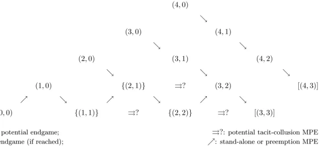
(17) without considering a potential reaction by its competitor. The mere ability to retaliate is not sufficient to sustain a tacit collusion equilibrium. We characterize below the conditions under which the retaliatory power is sufficient to offset the gain from deviating. If the firm to be punished is small, it does not lose as much from an increase in the capacity of its opponent as if it were bigger. This implies that retaliation, hence collusion, is likely to be easier between firms of similar size, while this explains also why the investment game cannot be over unless both firms hold strictly positive capacities. In what follows, firm asymmetry can only take the form of differences in current capacities and may be thought of as inherited from past moves in the industry development game. As discussed above, Lemma 1 provides only a partial characterization of value functions under alternative investment strategies. Completing the characterization requires knowledge of the continuation function  (·) and the appropriate trigger values. These can be determined when the game between the two firms is sufficiently near its end, in the sense of Proposition 1. Once the continuation value function is known in such situations, it is possible to characterize recursively the value function corresponding to the previous steps.. 3. Industry development. Assuming multiplicative demand separability and a finite (0) guarantees that a finite number of capacity units are eventually installed so that the investment game eventually comes to an end. Industry development possibilities are represented in Figure 1 as a tree whose nodes give the number of units held by firms. In order to investigate the level of competition at various points along an equilibrium path, it will be useful to focus on time intervals (or market development intervals) during which both firms invest once, either at the same time or at different times. In order to facilitate the analysis, we start with a series of simplified games designed in such a way that their solution is easily found; we then move on to the characterization of the general solution of the complete game by backward induction.. 14.

(18) . % (0 0) &. (1 0). (0 1). % & % &. (2 0)  (0  0 + 1) . . (0 + 1 0 + 1). %. (0  0 + 2). %. % &. . (1 1). & &. (0 + 2 0 + 1). %. (0 + 1 0 + 2). %. (0  0 + 3). %. . & & &. ( 0 + 3 0 + 1) (0 + 2 0 + 2) (0 + 1 0 + 3) (0  0 + 4) . (0 2).  . .  ( ). % &. ( + 1 ). %. (  + 1). %. & &. ( + 2 ). ( + 1  + 1). (  + 2). Figure 1: Industry capacity development tree While the figure indicates the possible investment sequences, it does not show any timing, or the market development thresholds at which capacity nodes may be reached. We characterize the capacity acquisition and the competition intensity prevailing at various stages (called episodes of capacity acquisition) of industry development: first, in the early stage when firms hold no capacity (Case 1); second, at a later stage, when firms hold similar (Case 2) or different (Case 3) capacities due to the unraveling of their respective investment strategies. Each of these cases is first examined under a choice of demand parameters such that the end of the game is “near”. By this we mean that demand assumptions ensure that, from the initial capacity nodes considered, a limited number of investments will lead to a situation where the investment game is over by Proposition 1. Once these particular games are solved, a slight relaxation of the demand assumptions used in cases 1-3 allows us to consider them as continuations of more general investment games whose solution can then be obtained by backward induction. This allows us to generalize the analysis (in Subsection 3.4) to arbitrary nodes in the industry development tree.. 15.

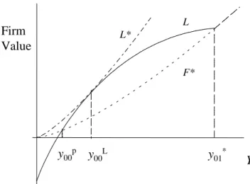
(19) 3.1. Case 1: No existing capacity. We start with a situation where initial capacities are zero. Let us assume generic demand to be such that unconstrained firms would produce at most one unit each in Cournot duopoly (recall Subsection 2.2), that is:. Assumption 2 0   ≤ 1. This assumption indicates that, although no firm holds capacity, we are close to the end of the investment game. It allows the monopoly output to exceed unity, so that the acquisition of more than one unit may be considered by any one firm, but it also implies that, if both firms hold one unit or more, the investment game is over by Proposition 1. Assumption 2 also implies that, whatever the (strictly) positive number of capacity units held by its opponent, a firm obtains instantaneous profit  11 once it invests in one unit or more; consequently, it will not acquire more than one unit if its opponent holds positive capacity. Therefore, the payoff from not investing immediately is (with 1 = 11 by Assumption 2).  (0 0 ) =. µ.  0. ¶ µ. ¶ 11 0 −   −. where  is the number of units acquired by the opponent before the firm acquires its first and single unit. The stopping problem faced by the firm is then:. ∗.  (0 0 ) = sup 0. "µ.  0. ¶ µ. 11 0 −  −. ¶#. (3). with solution:. ∗ ∗ = 01 = 0. −    ∀ ≥ 1 11  − 1. (4). Knowing this, the value for the competitor of acquiring at least one unit immediately at  = , and any ∗ can be computed explicitly. For example, if it number of additional units before  reaches the threshold 01. 16.

(20) acquires one unit immediately and abstains from any further investment, its value is, according to Lemma 1:10 10  (0 0 ) = − + − where. 11 ∗ − 01. µ.  ∗ 01. ¶. 11 − 10 ∗ ∗      01  −  01. (5). ∗ =  (1 0 ), since no more investment is forthcoming beyond 01 by Proposition 1. Similarly, if the. investment in the first unit is to take place in the future at 00  , then the value of the firm is:. (0 0 ) =. µ.  00. ¶ µ. 10 00 −  −. ¶. +. µ.  ∗ 01. ¶ µ. ¶ 11 − 10 ∗ 01  −. (6). Its maximum ∗ (0 0 ) with respect to 00 is reached at:.  = 00. −    10  − 1. (7). Figure 2 illustrates the functions  (0 0 ), ∗ (0 0 ) and  ∗ (0 0 ).. L. Firm Value. L*. F*. y00p y00L. y01*. Y. Figure 2: Firm values under alternative strategies.  ∗ It is straightforward to check from (3)—(6) that, within the interval (0 01 ), there exists a unique value 00 ,  , (0 0 )  corresponding to the intersection of  ∗ with  in Figure 2, such that for   [ =] 00   = inf{ ≥ 0 |  ≥ 00 }. [ =]  ∗ (0 0 ); the corresponding stochastic stopping time is 00 10 We leave it to the reader to adapt the formula and the rest of the argument for any number of units acquired by the first investor ∗ . For example, if the firm plans to acquire a second new unit at some  0 ,  ≤  0   ∗ , the candidate before the other one invests at 01 01       10 20 −10 0  21 −20 ∗ 0   ∗ where  value for  (0 0 ) is −  −  + 0  −  +    ≤  =  by Assumption 2. ∗ 21 11 01 01 −  − 01. If this value is higher than (5), then it gives the correct expression for  (0 0 ); if it is lower, then (5) is the appropriate expression. Note that the number of candidates to try is low as it cannot exceed the monopoly capacity under Assumption 2.. 17.

(21) We now determine the firms’ equilibrium strategies before any firm has invested, that is, in states of the form  ∗ , investing is for both firms a strictly dominated strategy while, for  ≥ 01 , delaying investment (0 0 ). If   00  ∗ ≤   01 , it is any further is also a strictly dominated strategy. To determine the equilibrium outcome when 00. helpful to consider what would happen if one of the firms were protected from preemption and could thus choose its optimal stand-alone investment date as a monopoly. Given a current industry-wide shock , the maximal expected payoff that this firm could then achieve by taking the lead is ∗ (0 0 ). This is strictly higher than  ∗ (0 0 ). However, in a MPE-compatible episode at (0 0 ), such a value gap cannot be sustained. If a firm   , then it is better-off preempting its rival at 00 − . This is true anticipates that its rival will first invest at 00    and 00 . When the industry-wide shock  is equal to 00 , the value of both firms is the for any  between 00. same, so each firm is indifferent between investing immediately and letting its rival invest while waiting to invest ∗ ∗ ∗ , at the stochastic time 01 = inf{ ≥ 0 |  ≥ 01 }. The following proposition is a transposition until  reaches 01. of Fudenberg and Tirole (1985, Proposition 2A) in a stochastic context..   there exists only one MPE-compatible episode outcome Proposition 2 Under Assumptions 1 and 2, if 0 ≤ 00  ∗  while the other firm waits until 01 to invest. Both of the investment game at (0 0 ): one firm invests at 00. times are stochastic and rents are equalized to the value of the second investor given by (3).. The simple MPE-compatible preemption episode in this case is characterized by intense competition. The first    00 , reflecting a partial capacity unit is installed earlier than under protection from preemption since 00. dissipation of monopoly rents (Posner, 1975; Fudenberg and Tirole, 1987). A rise in uncertainty increases both  ) in a MPE-compatible preemption episode.11  ∗ and  (see Figure 2) so that it may hasten investment (reduce 00. 3.1.1. Socially optimal investment timings. It is more difficult to compare the MPE-compatible episode outcome with the social optimum at (0 0 ). Specifically, let 0 = d(0)e be the minimum capital stock required to produce (0). The social planner’s problem is to find an increasing sequence of stopping times that solves: ⎧ ⎡ 0 ⎤⎫ Z   Z +1 ⎨ ⎬ X E ⎣ −  −1 ()  ⎦  sup ⎭ 1 ≤···≤0 ⎩  0 =1. 11 This possibility that increased volatility could hasten investment was pointed out by Mason and Weeds (2005) when firms are limited to one investment each; we generalize this result to multiple investments.. 18.

(22) where by convention 0 +1 = ∞. Standard computations imply that it is optimal for the social planner to invest in the first capacity unit when  reaches the investment trigger   such that:. . . Z. 0. 1. −1 ()  = ( − ).  , with the equality satisfied if From (7), we obtain   ≤ 00  in general. no obvious way to compare   and 00. However, let  =. R1 0. R1 0.   −1. (8).   −1 ()  = 10 . Since 00  00 as well, there is. −1 ()  − 10 represent the generic net consumer surplus on the first capacity unit;. it only depends on the slope of the demand function on [0 1]. In particular,  = 0 if the inverse demand curve    00 . Consequently, for any set of parameters is a step function, −1 () = −1 (de), implying that   = 00   and 00 , there exists a set of demand functions  () satisfying Assumption 1 such that  is small defining 00  . This proves the following proposition. enough for   to be higher than 00.   and 00 , there exists a set of demand functions  () Proposition 3 For any set of parameters determining 00. satisfying Assumption 1 such that the first industry investment occurs earlier in the MPE-compatible preemption episode than would be socially optimal at (0 0 ).. Leahy (1993) discusses the timing of entry. In a model of industry capacity investments where investment units are of negligible size, he shows that the timing of investments is socially optimal under perfect competition, no matter what the demand function is. But in a duopoly, preemption accelerates entry. However, lumpy indivisible capacity units also imply that perfect competition is not socially optimal in general: unlike the social planner, competitive firms do not consider the consumer surplus when they compute profits, so that they underestimate the benefits of entry relative to the social planner. This factor postpones entry relative to the social optimum and may dominate the preemption effect when the net-of-price consumer surplus is big; it is small when the slope of the inverse demand is small and vanishes altogether when the inverse demand is a step function. The result that the first industry investment may occur earlier under duopoly than is socially optimal does not depend on the market size assumption  = 1. In particular it applies in the generalized treatment presented in Section 3.4 below.. 19.

(23) 3.2. Case 2: Symmetric positive capacities. Let us now investigate the role of existing capacity, starting in this section with situations where firms have identical positive capacities, as illustrated by the subgame starting at node ( ) in Figure 1. As in the previous subsection, we will assume that the firms hold a capacity lower than the unconstrained short-run Cournot output, which implies that both firms are initially capacity constrained and that a firm remains constrained if its opponent invests:. Assumption 3 0   −  ≤ 1. Assumption 3 is compatible with an unconstrained monopoly output exceeding  + 1, so that it does not rule out investments exceeding one unit, thereby allowing a firm to get ahead by more than one unit. It does imply that the end of the game is not too far in the sense that, by Proposition 1, the game is over once both firms have acquired at least one more unit. To simplify exposition without loss of generality, we take  = 1 Then Assumption 3 implies that 21  11 , 22  12 , and 2 = 22 = 2 , ∀ ≥ 2. When considering a new investment, firms will now take into account the consequences on the profits they derive from their existing capacity. We will show that, as a result of the cannibalism effect, MPE exhibiting tacit collusion at that node ( ) = (1 1) may exist besides the MPE with preemption, provided that either late joint investment or no more investment dominates preemption over the whole relevant market development range.. 3.2.1. MPE-compatible preemption episode at ( )    0. A MPE-compatible preemption episode at ( )    0 always exists along any MPE investment path. Let  = 1 Indeed, assume that one of the firms has taken the lead by acquiring at least one new unit, bringing its total capacity to  ≥ 2. For its rival, whatever the number of units held by the first investor, it is a dominant strategy by Assumption 3 to acquire one and only one unit at the market development threshold determined by the following stopping-time problem: for   1 , ". 1  ∗ (1  ) = sup +  − 1. µ.  1. 20. ¶ µ. 22 − 1 1 −  −. ¶#. . (9).

(24) that is, at:. ∗ = 1. −    22 − 1  − 1. (10). The situation is similar to the case with no initial capacity, except that the trigger value at which the second investor invests depends on the number  of units held by the first investor. The higher  is, the earlier the second investor will invest because its profits 1 , while he is waiting, are lower, the higher  is. The firm that invests first, whether it acquires one single unit or more units, understands the implications of its investment decision on the behavior of its competitor, so that  (1 1 ) can be computed explicitly. For ∗ is, for  = 1: example, if the early investor acquires only one unit, its payoff at the current level of  ≤ 1. 21  (1 1 ) = − + −. µ.  ∗ 12. ¶ µ. ¶ 22 − 21 ∗    −  12. (11). As before, if the firm could choose the investment threshold in the absence of any threat of preemption, the maximum ∗ (1 1 ) with respect to , for  = 1, would be reached at:12.  11 =. −    21 − 11  − 1. But under a preemption threat, it is not possible for the firm to achieve a value of  exceeding  ∗ ; it cannot wait   ; the best it can do is to invest at the trigger level 1 at which  (1 1 ) =  ∗ (1  ), so until  reaches 1. that rents are equalized. The following result parallels Proposition 2.. Proposition 4 [MPE-compatible preemption episode at ( )    0] Under Assumptions 1 and 3, the investment game has a MPE-compatible preemption episode at node ( ) such that, letting  = 1, one firm invests  ∗ , while the other firm invests when  reaches 1 . when  reaches 1. In this MPE-compatible episode, the threat of preemption leads to rent equalization and thus to the complete dissipation of any first-mover advantage. However, with positive capacities, the preemption equilibrium episode may not be the unique MPE-compatible episode at positive capacity node ( ), as we shall now see. 12 Again, the reader can adapt the candidate expressions for  (1 1 ), with  ∗ given by (10), for any new capacity purchase 1 exceeding one unit (  2). The highest such candidate gives  (1 1 ). It is certain to exist because, as shown in the proofs, the ∗ ∗ . candidate for  corresponding to  = 1 exceeds  (1 1 ) for some range of  values lower than 12. 21.

(25) 3.2.2. MPE-compatible tacit collusion episode at ( )    0. As in Fudenberg and Tirole (1985), the fact that the firms hold strictly positive capacities gives rise to the possibility of a different type of MPE-compatible episode. In this alternative, the strategies involved consist in “coordinating” on a high joint investment threshold or in abstaining from investing forever, thereby postponing the rise in industry capacity and thus increasing firms’ values. Note that short-run output decisions are still determined according to Cournot competition. Tacit collusion is achieved through investment timings, not through production decisions. This implies that firms can sustain a tacit collusion outcome through investing simultane ∗ exceeding 12 . Indeed if one of the firms ously, rather than at different times, and by doing so at a threshold 12 ∗ ∗ , the other firm’s unique optimal continuation strategy would be to invest at 12 . were to invest at some   12  as shown in the analysis of the MPE-compatible preemption episode This can be part of an MPE only if  = 12 ∗  then a dominant strategy for the other characterized above. Alternatively, if it were to invest at some  ≥ 12. firm would be to follow suit and invest at the same time. Since simultaneous investments of one unit imply, by Assumption 3, that both firms then hold more capacity than the unconstrained Cournot output, they will not acquire more than one unit. Furthermore, the game is then over by Proposition 1. Postponing investment or not investing restricts output. In that sense the tacit collusion equilibrium episode is reminiscent of the early-stopping equilibrium of Fudenberg and Tirole (1983) and of the tacitly collusive underinvestment equilibria of Nocke (2007) described earlier.13 Suppose that the firms could commit to invest simultaneously at some (random) future date or to abstain from investing forever. Given a current industry-wide shock , the expected payoff that they could achieve in this way is, according to Lemma 1: 11 +  (1 1 ) = −. µ.   11. ¶ µ. ¶ 22 − 11   −   −  11. (12). 13 However, Fudenberg and Tirole considered a dynamic game with downward sloping reaction functions in continuous investment levels. Such reaction functions imply that capacity is always scarce which may lead to a race to invest aimed at inducing the competitor to reduce its investment. We consider a dynamic game in lumpy investment. Once the capacity of the larger firm exceeds a certain level, the smaller firm is able fully to exploit its new capacity irrespective of any reaction by the larger firm; as a result the larger firm cannot indefinitely induce postponement of the smaller firm’s investment by acquiring additional capacity. In that sense, even a preemption episode, where one firm invests early while the other firm waits, does not qualify as a race since both firms end up with the same value.. 22.

(26)  ∗ If 22  11 ,  (1 1 ) has a maximum with respect to 11 , denoted  ∗ (1 1 ), at 11 :. ∗ = 11. −  −  ∗  =   12  22 − 11  − 1 22 − 12  − 1. (13). ∗ ∗ = inf{ ≥ 0 |  ≥ 11 } as the corresponding investment (stochastic) timing. If 22 ≤ 11 ,  (1 1 ) with 11. attains a maximum of. 11 − . ∗ ∗ by letting 11 = ∞ (tacit collusion by inaction), in which case 11 = ∞. Clearly if. ∗ , tacit collusion cannot occur in equilibrium since each firm then has  (1 1 ) exceeds  ∗ (1 1 ) at any  ≤ 11. an incentive to deviate and invest earlier. Hence,. Proposition 5 [MPE-compatible tacit collusion episode at ( )    0] Under Assumptions 1 and 3 and letting    = 1, if 0 ≤ 11. 1. A necessary and sufficient condition for the existence of a MPE-compatible tacit collusion episode at ( ) ∗ . If this inequality is strict for all such , there exists a continuum is  (1 1 ) ≤  ∗ (1 1 ) ∀  12  in the range of (MPE-compatible tacit collusion episodes, indexed by their joint investment triggers 11 ∗ ∗ ∗ ], where 12 ≤   ≤ 11 . [   11. 2. Rents are equalized in each MPE-compatible tacit collusion episode and exceed the rents in the MPEcompatible preemption episode at the same node; the Pareto optimal MPE-compatible tacit collusion episode corresponds to the joint-profit maximizing investment rule under the constraint that firms invest simultaneously if they do.14 In this joint-profit maximizing MPE-compatible tacit collusion episode, each firm invests in one capacity unit with intensity:. 1 (1 1 ) = − 1 (1 1 ) =. ⎧ ∗ ⎪ ⎪ 0 if  ∈ [0 11 ) ⎪ ⎨. ⎪ ⎪ ⎪ ⎩ 1 if  ∈ [ ∗  ∞) 11. 3. If 22  11 , the Pareto optimal MPE-compatible tacit collusion episode has both firms investing when  ∗ ∗ reaches 11 ; otherwise, it is such that neither firm ever invests as 11 = ∞.. Propositions 2 and 5 highlight the role of existing capacity in the exercise of market power. A firm that holds no capacity has no incentive to restrain output and thus a MPE-compatible tacit collusion episode cannot 14 In the absence of that constraint, joint-profit maximization would involve sequential investments. Such an investment sequence cannot be sustained as an MPE-compatible outcome as it would generate a strictly higher expected payoff for the first investor and would, therefore, be subject to preemption.. 23.

(27) exist if one firm has zero capacity (Proposition 2). In the language of contestability, this says that the level of contestability is stronger when the contesting firm is not yet active. Moreover, the mere existence of an incentive to tacitly collude is not enough to guarantee that tacit collusion is sustainable in equilibrium: firms must also follow investment strategies such that a deviation from the tacit collusion outcome would trigger a reaction leading to a new equilibrium with a lower value for the deviating firm. This “punishment” is made difficult because our assumption of a Cournot production equilibrium in any period implies that restraining output can only be achieved by postponing capacity investments in the industry. It follows, in particular, that the joint investment trigger in any MPE-compatible tacit collusion episode must be higher than both triggers in the MPE-compatible preemption episode characterized in Proposition 4. Moreover, a firm becomes more vulnerable to a deviation by its competitor once the trigger value for the first investment  and until  reaches the threshold for the second in the preemption equilibrium has been crossed: once   11. investment, a deviation yields the defector a higher rent  (·) than the rent  ∗ (·) obtained by its competitor who ∗ . Therefore, the rents  ∗ (·) under tacit collusion must be attractive enough would then invest optimally at 12 ∗  (Proposition 5(2)) to beat such defection at any level of  preceding 12. Proposition 5 provides a necessary and sufficient condition for the existence of MPE-compatible tacit collusion episodes at ( )  This condition implies restrictions on the components of  (1 1 ) and  ∗ (1 1 ): first, the four profit values  determined by the non-stochastic component of demand  (·) under Cournot competition; second, the parameters underlying real option values, that is, the value of  as determined by the discount rate  as well as the drift  and the volatility  of the stochastic demand growth process. ∗ e ( ) ≡ {(11  12  22  21 ) |  ∗ (1 1 ) −  (1 1 ) ≥ 0 ∀  12 } be the set of  quadruples for which Let Λ. MPE-compatible tacit collusion episodes exist given  and . The following proposition states that this set is. e ( ) = Λ()), and larger in industries with higher volatility, faster non-empty, independent of  (that is, Λ. demand growth and lower cost of capital (that is, Λ ( 0 ) ⊂ Λ () iff    0 ).. Proposition 6 [MPE-compatible tacit collusion episodes: existence] Under Assumptions 1 and 3,. 1. There exists a set of market parameters guaranteeing the existence of MPE-compatible tacit collusion episodes at ( )    0. 2. This set is independent of the investment cost  of a capacity unit. 24.

(28) 3. It is larger, the higher demand volatility is, the faster market growth is, and/or the smaller the discount rate or cost of capital is.. As we know from the real option literature, increased volatility raises the option value of an irreversible investment under no preemption threat: the firm increases its investment threshold to reduce the probability that the stochastic process reverts to undesirable levels after the firm has invested. The flexibility to do so increases the value of the firm and the more so, the higher the volatility. Such an effect is also present here. There is another effect of volatility: an increase in volatility raises firm value more under tacit collusion than under preemption, thus favoring the emergence of the former. The reason comes from both timing and discounting. Tacit collusion involves higher investment thresholds (hence longer delays), while an increase in volatility amounts to a lower discount rate (recall that  decreases with volatility ) because it raises the probability that a given threshold value of  will be reached in a given time span. Although instantaneous profits are always independent of , the discounted value of the profit flows corresponding to each equilibrium does depend on : letting  = 1, ³ ´ ³ ´  ∗ and ∗ and, since 11  12  the (state space) discount factors used in (12) and (11) are respectively  11. 12. the former increases more than the latter when  decreases, that is, when volatility increases.. To put it differently, the benefits of restraining output through delaying investments occur in the distant future, that is, in a higher state of market development, while the benefits from deviating occur in the immediate future. Other things equal, higher volatility gives relatively more weight to the distant future, contrary to conventional wisdom whereby increased volatility, because it warrants a risk premium, amounts to an increase in the discount rate. The intuition for such effects of the (time) discount rate and the market growth rate is similar: a lower discount rate favors future payoffs and a larger expected growth rate raises future prospects relative to immediate ones. Hence, both favor the existence of tacit collusion through a lower .. 3.3. Case 3: Different capacities. While we have shown that existing capacity is a necessary condition for tacit collusion between identical firms, capacity is also often said to play a role as a barrier to entry and thus can be used as a way to acquire and. 25.