HAL Id: insu-01508081
https://hal-insu.archives-ouvertes.fr/insu-01508081
Submitted on 13 Apr 2017
HAL is a multi-disciplinary open access
archive for the deposit and dissemination of
sci-entific research documents, whether they are
pub-lished or not. The documents may come from
teaching and research institutions in France or
abroad, or from public or private research centers.
L’archive ouverte pluridisciplinaire HAL, est
destinée au dépôt et à la diffusion de documents
scientifiques de niveau recherche, publiés ou non,
émanant des établissements d’enseignement et de
recherche français ou étrangers, des laboratoires
publics ou privés.
Infrared Radiometer (IIR) calibration and stability
through simulated and observed comparisons with
MODIS/Aqua and SEVIRI/Meteosat
Anne Garnier, Noëlle A. Scott, Jacques Pelon, Raymond Armante, Laurent
Crépeau, Bruno Six, Nicolas Pascal
To cite this version:
Anne Garnier, Noëlle A. Scott, Jacques Pelon, Raymond Armante, Laurent Crépeau, et al..
Long-term assessment of the CALIPSO Imaging Infrared Radiometer (IIR) calibration and stability through
simulated and observed comparisons with MODIS/Aqua and SEVIRI/Meteosat. Atmospheric
Mea-surement Techniques, European Geosciences Union, 2017, 10 (4), pp.1403-1424.
�10.5194/amt-10-1403-2017�. �insu-01508081�
www.atmos-meas-tech.net/10/1403/2017/ doi:10.5194/amt-10-1403-2017
© Author(s) 2017. CC Attribution 3.0 License.
Long-term assessment of the CALIPSO Imaging Infrared
Radiometer (IIR) calibration and stability through simulated and
observed comparisons with MODIS/Aqua and SEVIRI/Meteosat
Anne Garnier1,2, Noëlle A. Scott3, Jacques Pelon4, Raymond Armante3, Laurent Crépeau3, Bruno Six5, and Nicolas Pascal6
1Science Systems and Applications, Inc., Hampton, VA 23666, USA 2NASA Langley Research Center, Hampton, VA 23681, USA
3Laboratoire de Météorologie Dynamique, Ecole Polytechnique–CNRS, 91128 Palaiseau, France 4Laboratoire Atmosphères, Milieux, Observations Spatiales, UPMC–UVSQ–CNRS, 75252 Paris, France 5Université Lille 1, AERIS/ICARE Data and Services Center, 59650 Lille, France
6Hygeos, AERIS/ICARE Data and Services Center, 59650 Lille, France
Correspondence to:Anne Garnier ([email protected]) Received: 13 October 2016 – Discussion started: 14 November 2016
Revised: 6 March 2017 – Accepted: 21 March 2017 – Published: 13 April 2017
Abstract. The quality of the calibrated radiances of the medium-resolution Imaging Infrared Radiometer (IIR) on-board the CALIPSO (Cloud-Aerosol Lidar and Infrared Pathfinder Satellite Observation) satellite is quantitatively evaluated from the beginning of the mission in June 2006. Two complementary “relative” and “stand-alone” ap-proaches are used, which are related to comparisons of mea-sured brightness temperatures and to model-to-observations comparisons, respectively. In both cases, IIR channels 1 (8.65 µm), 2 (10.6 µm), and 3 (12.05 µm) are paired with the Moderate Resolution Imaging Spectroradiometer (MODIS)/Aqua Collection 5 “companion” channels 29, 31, and 32, respectively, as well as with the Spinning Enhanced Visible and Infrared Imager (SEVIRI)/Meteosat companion channels IR8.7, IR10.8, and IR12, respectively. These pairs were selected before launch to meet radiometric, geometric, and space-time constraints. The prelaunch studies were based on simulations and sensitivity studies using the 4A/OP ra-diative transfer model and the more than 2300 atmospheres of the climatological Thermodynamic Initial Guess Retrieval (TIGR) input dataset further sorted into five air mass types. Using data from over 9.5 years of on-orbit operation, and following the relative approach technique, collocated mea-surements of IIR and of its companion channels have been compared at all latitudes over ocean, during day and night,
and for all types of scenes in a wide range of brightness tem-peratures. The relative approach shows an excellent stability of IIR2–MODIS31 and IIR3–MODIS32 brightness temper-ature differences (BTDs) since launch. A slight trend within the IIR1–MODIS29 BTD, that equals −0.02 K yr−1on av-erage over 9.5 years, is detected when using the relative ap-proach at all latitudes and all scene temperatures. For very cold scene temperatures (190–200 K) in the tropics, each IIR channel is warmer than its MODIS companion channel by 1.6 K on average. For the stand-alone approach, clear sky measurements only are considered, which are directly com-pared with simulations using 4A/OP and collocated ERA-Interim (ERA-I) reanalyses. The clear sky mask is derived from collocated observations from IIR and the CALIPSO li-dar. Simulations for clear sky pixels in the tropics reproduce the differences between IIR1 and MODIS29 within 0.02 K and between IIR2 and MODIS31 within 0.04 K, whereas IIR3–MODIS32 is larger than simulated by 0.26 K. The stand-alone approach indicates that the trend identified from the relative approach originates from MODIS29, whereas no trend (less than ±0.004 K yr−1) is identified for any of the IIR channels. Finally, using the relative approach, a year-by-year seasonal bias between nighttime and daytime IIR– MODIS BTD was found at mid-latitude in the Northern Hemisphere. It is due to a nighttime IIR bias as determined
by the stand-alone approach, which originates from a cali-bration drift during day-to-night transitions. The largest bias is in June and July when IIR2 and IIR3 are warmer by 0.4 K on average, and IIR1 is warmer by 0.2 K.
1 Introduction
The Cloud-Aerosol Lidar and Infrared Pathfinder Satel-lite Observation (CALIPSO) satelSatel-lite (Winker et al., 2010), launched in April 2006, includes a payload of three instru-ments, the Cloud-Aerosol Lidar with Orthogonal Polariza-tion (CALIOP), a visible wide-field camera, and the Imag-ing Infrared Radiometer (IIR). The IIR was built in France by the Centre National d’Études Spatiales (CNES), the So-ciété d’Études et de Réalisations Nucléaires (SODERN), and Institut Pierre Simon Laplace (IPSL) (Corlay et al., 2000). It includes three spectral bands in the thermal infrared at-mospheric window, at 8.65 µm (IIR1), 10.6 µm (IIR2), and 12.05 µm (IIR3) with bandwidths of 0.85, 0.6, and 1 µm, spectively. These three channels were chosen to optimize re-trievals of ice cloud properties in synergy with collocated observations from the CALIOP lidar (Garnier et al., 2012, 2013).
It is now well recognized by the international community that to be fully useful for climate and meteorological applica-tions, satellite observations require quality control during the instrument’s lifetime. Indeed, any systematic error or spuri-ous trend not identified in the calibrated radiances may in-duce artifacts in the retrieved variables. In the mid-1990s, the NOAA/NASA Pathfinder Program and, later in 2005, the Global Space-based Inter-Calibration System (GSICS) initi-ated international collaborative efforts to improve and har-monize the quality of observations from operational weather and environmental satellites in order to create climate data records (e.g., Goldberg et al., 2011). A recent update on the GSICS vision is given in a 2015 World Meteorological Or-ganization (WMO) report (GSICS, 2015).
In this paper, IIR observations since launch are monitored and characterized using two complementary approaches, which are the heritage of the processing of numerous years of satellite radiances for the restitution of climate variables (Chédin et al., 1985, and papers following on similar top-ics referenced and regularly updated at http://ara.abct.lmd. polytechnique.fr/index.php?page=publications). The moni-toring of observational and computational biases or trends over long periods of time started with the NOAA/NASA TIROS Operational Vertical Sounder (TOVS) Pathfinder Pro-gram (Scott et al., 1999). Since then, it has been implemented for more recent hyperspectral sounders, namely the Atmo-spheric Infrared Sounder (AIRS) on-board the Aqua satel-lite since 2003, and since 2007 for the Interféromètre Atmo-sphérique de Sondage Infrarouge (IASI) on the MetOpA and
MetOpB satellites in cooperation with CNES (e.g., Jouglet et al., 2014) within the frame of its GSICS activities.
The first approach, called the “relative” approach, is based on a channel to channel intercomparison of radiances, fur-ther converted into equivalent brightness temperatures, with collocated measurements in companion channels of com-panion instruments under controlled conditions. The rela-tive approach, sometimes referred to as the “inter-channel” or “inter-calibration” approach, was initially developed in a geostationary–low Earth orbit (GEO–LEO) combination for the calibration of Meteosat-1, based on space and time collo-cations with TOVS on the NOAA TIROS-N series (Bériot et al., 1982). The second approach, called the “stand-alone” ap-proach, is based on comparisons between measured and sim-ulated brightness temperatures for each companion channel of each companion instrument. The two approaches are com-plementary: the inter-calibration approach studies the behav-ior of one channel relative to its companion regardless of the underlying clear or cloudy scene and therefore allows for the study of a wide range of brightness temperatures. The stand-alone approach screens each channel of each instrument, in-dividually, for clear sky scenes and helps to identify which channel deviates from the other(s). In this study, the clear sky mask is derived from collocated observations from the IIR and CALIOP.
The IIR companion instruments chosen for this study are the Moderate Resolution Imaging Spectroradiometer (MODIS) on-board Aqua and the Spinning Enhanced Visi-ble and Infrared Imager (SEVIRI) on-board the geostationary second generation satellites Meteosat 8, 9, and 10. Both the MODIS and SEVIRI instruments, in operation since 2002 and 2004, respectively, include medium-resolution spectral bands similar to IIR channels.
An assessment of IIR radiances after 9.5 years of nearly continuous operation is presented, thereby updating the first results published in Scott (2009). This paper presents a brief description of the IIR instrument in Sect. 2, with prelaunch studies for the selection of IIR companion instrument and channels identified in Sect. 3, and the implementation of the relative and stand-alone approaches described in Sect. 4. Re-sults and findings from the relative and the stand-alone ap-proaches are presented in Sect. 5 and Sect. 6, respectively, and our assessment is summarized in the last section.
2 The IIR/CALIPSO instrument
The entire CALIPSO payload flies in a near-nadir, down-looking configuration, with a 0.3◦angle off-nadir in the for-ward direction. The off-nadir angle was increased to 3◦at the end of November 2007 to reduce specular reflections from horizontally oriented ice crystals in CALIOP observations (Hu et al., 2009). The IIR instantaneous field of view is ±2.6◦ or 64 × 64 km on the ground, with 1 km size pixels. Thus, the viewing angles from nadir range from 0 to 3◦until
Novem-ber 2007 and from 1 to 6◦after the CALIPSO payload pitch change, which is not expected to have any identifiable impact on the observations.
The IIR instrument (Corlay et al., 2000) includes three fil-ters which are mounted on a rotating wheel for sequential ac-quisition within their respective spectral bands. The sensor is an uncooled microbolometer array (U3000) manufactured by Boeing and also implemented in the IASI instruments. IIR is regularly calibrated in flight using images of a temperature-monitored warm blackbody source (at about 295 K) and from cold deep space (about 4 K) views. For each spectral band and for each pixel in the image, cold space views are used to determine the offset of the detection system, and images from the calibration blackbody source at known tempera-tures are used to retrieve the gains. The linearity of the de-tection system was verified before launch for scene tempera-tures ranging between 215 and 320 K, and the gain retrieved from the warm calibration source is directly applied to cal-ibrate the earth view images. Instrument spectral response functions (ISRFs) for each band were established by CNES before launch and are available upon request.
The overall calibration accuracy of the IIR measurement is specified to be better than 1 K in all channels. In-flight performances were assessed by CNES at the beginning of the mission (Trémas, 2006; Tinto and Trémas, 2008). The in-flight short-term gain stability was found to be better than 0.1 K of equivalent brightness temperature, except during the day-to-night transitions, during which the gain varies by up to 0.45 K. The in-flight noise equivalent differential temper-ature (NedT) at 210 K was between 0.2 and 0.3 K, similar to values measured before launch and better than the specified value of 0.5 K. The NedT is of the order of 0.1 K at 250 K.
The calibrated radiances are reported in the CALIPSO Version 1 IIR Level 1B products (Vaughan et al., 2015) avail-able from the Atmospheric Science Data Center of the NASA Langley Research Center and at the AERIS/ICARE data cen-ter in France. They are resampled and regiscen-tered on a 1 km resolution unique grid centered on the CALIOP ground track, at sea level, with a 69 km swath. The products are organized by separating the daytime and nighttime portions of an or-bit to match the definition chosen for CALIOP and thereby facilitate synergetic analyses. Because the lidar is very sen-sitive to daylight background noise, the nighttime portion of the orbit is when the solar elevation angle at earth surface is less than −5◦(Hunt et al., 2009).
3 Method and prelaunch studies
Both the relative and the stand-alone approaches require (i) companion instruments that offer the best possible spa-tiotemporal coincidences with IIR (primarily in order to see the same scenes simultaneously), and (ii) companion channels presenting close characteristics in terms of spec-tral coverage and spatial resolution. These constraints have
oriented our choice towards two companion instruments: MODIS/Aqua and SEVIRI/Meteosat.
3.1 Description of companion instruments
MODIS/Aqua and SEVIRI/Meteosat in-flight performances have been extensively characterized (Xiong et al., 2015; EU-METSAT, 2007a, and references herein). The main instru-mental characteristics of interest for comparison with IIR are summarized in Table 1 and are detailed in the following sub-sections.
3.1.1 MODIS/Aqua
The first companion instrument chosen for this study, MODIS/Aqua, includes three medium-resolution spectral bands in the thermal infrared window (29, 31, and 32), with 1 km spatial resolution of interest for comparisons with IIR. Furthermore, both Aqua and CALIPSO, which is nominally positioned 73 s behind Aqua, have been flying in forma-tion with other satellites of the A-Train (Stephens et al., 2002) since June 2006. The A-Train satellites follow a Sun-synchronous polar orbit at 705 km altitude with a 98.2◦ in-clination. CALIPSO measurements provide global cover-age between 82◦N and 82◦S. There is a 16-day repetition cycle, with an equator crossing time at about 13:35 local time. CALIPSO is controlled according to a customized grid shifted by 7 min 44 s local time from the nominal Worldwide Reference System-2 (WRS-2) grid used by Aqua, or 215 km eastward at the equator crossing. Due to the relative posi-tions of the CALIPSO and Aqua satellites in the A-Train, the MODIS 2330 km swath always covers the IIR 69 km swath. The viewing angles for the MODIS pixels collocated with the IIR swath vary with latitude, as illustrated in Fig. 1, which shows histograms of MODIS viewing angles for six 30◦ lat-itude bands for clear sky pixels over ocean in July 2014. The MODIS viewing angle is largest at the equator and ranges from 12 to 20◦at 0–30◦latitude in both hemispheres. It de-creases progressively as latitude inde-creases, to be mostly be-tween 8 and 18◦at 30–60◦north and south and less than 12 at 60–82◦N. The pixels over ocean south of 60◦S are actually north of about 70◦S due the presence of the Antarctic con-tinent, which explains why histograms at 82–60◦S exhibit larger angles on average than those at 60–82◦N. These ge-ometries of observation are accounted for in the simulations. 3.1.2 SEVIRI/Meteosat
Comparing IIR and MODIS/Aqua observations, both from the A-Train, ensures a very large sampling for statistical anal-yses. A complementary view is available through compar-isons with SEVIRI on-board the geostationary second gener-ation Meteosat satellites. SEVIRI provides radiometric data every 15 min in three spectral bands in the thermal infrared (channels IR8.7, IR10.8, and IR12) with a 3 km resolution at the sub-satellite point, which is at 0◦in both latitude and
lon-Table 1. Main characteristics of the instruments and channels considered for this study.
Instrument IIR MODIS SEVIRI
Platform CALIPSO AQUA Meteosat 8, 9, and 10 Orbit LEO, A-Train LEO, A-Train GEO
73 s behind AQUA
Temporal coverage Sun-synchr. 13:43 Sun-synchr. 13:35
16-day repetition 16-day repetition 15 min repeat cycle Geographical From WRS-2 grid WRS-2 grid
coverage for the study Lat.: 82◦S–82◦N Lat.: 82◦S–82◦N Lat.: 10◦S–10◦N All longitudes All longitudes Long.: 10◦W–10◦E Spectral bands #1: 8.2–9.05 µm #29: 8.4–8.7 µm IR8.7: 8.3–9.1 µm
#2: 10.35–10.95 µm #31: 10.78–11.28 µm IR10.8: 9.8–11.8 µm #3: 11.6–12.6 µm #32: 11.77–12.27 µm IR12: 11.0–13.0 µm
Swath 69 km 2330 km Full disk
Resolution 1 km 1 km 3 km sub-satellite NedT 0.2–0.3 K @ 210 K < 0.025 K < 0.12 K
0.1 K @ 250 K (Xiong et al., 2015) (EUMETSAT, 2007a) Specification: < 0.5 K
Figure 1. Histograms of MODIS viewing angles for clear sky pixels collocated with the IIR swath over ocean in July 2014. Top row from left to right: 60–82, 30–60, 0–30◦N. Bottom row from left to right: 82–60, 60–30, and 30–0◦S.
gitude for the prime satellites. SEVIRI data are from three different prime geostationary satellites since June 2006: Me-teosat 8 until 11 April 2007, then MeMe-teosat 9 until 21 Jan-uary 2013, and currently Meteosat 10. IIR and SEVIRI are best compared when SEVIRI viewing angles are smaller than 10◦to be close to IIR quasi-nadir observations, therefore, at latitudes between 10◦N and 10◦S and longitudes between 10◦W and 10◦E.
3.2 Selection of IIR, MODIS, and SEVIRI companion channels
The IIR companion channels were chosen before launch among the various spectral channels of MODIS/Aqua and SEVIRI/Meteosat following a specific procedure. For each IIR channel, the selected MODIS or SEVIRI companion channel is the one that not only minimizes the brightness temperature differences (BTDs) with IIR, but also shows a similar sensitivity to the atmosphere and to the surface. This evaluation was conducted before launch by simulat-ing the IIR and candidate companion channels ussimulat-ing the forward radiative transfer model 4A (4A: Automatized
At-mospheric Absorption Atlas) and more than 2300 atmo-spheres from the Thermodynamic Initial Guess Retrieval (TIGR) input dataset. MODIS/Aqua ISRFs can be retrieved from the MODIS Characterization Support Team website (http://mcst.gsfc.nasa.gov/calibration/parameters) and SE-VIRI/Meteosat ISRFs from the EUMETSAT MSG Calibra-tion website (http://www.eumetsat.int/website/home/Data/ Products/Calibration/MSGCalibration/index.html). In addi-tion to the radiative coherence of the different pairs of chan-nels, the quality of the comparisons performed for both the relative and the stand-alone approaches is based on the high-est possible homogeneity of the observed surfaces and of the atmospheric optical paths. Differences in the spectral posi-tion and shape of the ISRFs can induce differences in surface emissivity. Furthermore, regardless of the perfection of the space-time collocation of the different instruments, the emit-ting surface may still be observed under different conditions. This is inherently related to the difference in the pixel size of each instrument as well as to the difference in the optical paths resulting from different viewing angles. Handling these differences is more difficult over land where altitude and na-ture of the ground contribute to enhance the inhomogeneity of the observed scenes. We have chosen to minimize these issues by restricting our study to observations over ocean. It is worthwhile to note that this choice allows a robust calibra-tion assessment, in a wide range of brightness temperatures, at most latitudes and at any season, which is compatible with the aim of our study. Future work will include analyses at the highest latitudes, which are currently not examined be-cause they are covered by ice, and analyses in extreme condi-tions of land surface temperatures. The simulated BTDs be-tween IIR and the selected companion channels are shown in Sect. 3.2.3, after a brief description of the simulation model and of the auxiliary datasets in Sect. 3.2.1 and 3.2.2. 3.2.1 The forward radiative transfer model: 4A The radiative transfer model used at all stages of this study is 4A/OP, the operational version of 4A, adapted and main-tained by NOVELTIS (http://4aop.noveltis.com/) in collab-oration with CNES and Laboratoire de Météorologie Dy-namique (LMD). The 4A model is a fast and accurate line-by-line (LBL) radiative transfer model initially developed at LMD (Scott and Chédin, 1981). As recalled in Anthony Vin-cent and Dudhia (2017), 4A was among the pioneer radia-tive transfer models to bypass LBL processing time by cal-culating once and for all a set of compressed look-up tables (LUTs) of monochromatic optical depths. These LUTs are generated by the nominal line-by-line STRANSAC model (Scott, 1974; Tournier et al., 1995) coupled to the Gestion et Étude des Informations Spectroscopiques Atmosphériques (GEISA) spectroscopic database. The 4A model generates transmittances, radiances, and jacobians (Chéruy et al., 1995) for any instrumental, spectral, and geometrical configuration (ground, airborne, and satellite).
The 4A model has a long history of validation within the frame of the international radiative transfer community. From the very beginning, most of the validation results have been extensively discussed in a number of intercompari-son exercises and in particular during the Intercompariintercompari-son of Transmittance and Radiance Algorithms (ITRA) work-ing groups – 1983, 1985, 1988, and 1991 – of the Inter-national Radiation Commission (Chédin et al., 1988) and during the Intercomparison of Radiation Codes in Climate Models (ICRCCM) campaigns (Luther et al., 1988). More recently, observations from hyperspectral sounders such as AIRS and IASI have led to even more extensive valida-tions, again within the frame of international observation campaigns or working groups, among them the International TOVS Study Conferences (ITSC) and the IASI Sounding Science Working Group (ISSWG). The 4A model is the of-ficial code selected by CNES for calibration and validation activities of the IASI, Merlin (https://merlin.cnes.fr), and Mi-croCarb (https://microcarb.cnes.fr) missions. A detailed de-scription of the protocol and of the results of the interactive validation of GEISA and 4A/OP may be found in Armante et al. (2016).
Throughout the 9.5 years of IIR operation analyzed here, we have used a static version of 4A (2009 version) in order to avoid undesirable, however smooth, jumps. The LUTs were generated with STRANSAC coupled to the 2011 version of GEISA (Jacquinet-Husson et al., 2011). The 4A/OP model is in “down–up” mode, which means that the emission by the surface, the upwelling atmospheric radiation, and the reflec-tion at the surface of the downwelling atmospheric radiareflec-tion are taken into account, modulated by the emissivity or the reflectivity. The attenuated reflected downward radiance has been computed using a constant diffusivity factor. This ap-proximation avoids computing a large number of downward radiances (and, above all, the computation of a large number of transmittance functions) corresponding to a large number of incident angles as well as integrating overall these angles. Such an approximation for the integration over the angle is usual in radiative transfer calculations: it was suggested as early as 1942 by Elsasser. Later on, tests on the validity of this approximation have been presented by Rodgers and Wal-shaw (1966), Liu and Schmetz (1988), Turner (2004), and many others. A value of 53◦is used here for the computation of the downwelling reflected radiances. Simulations are con-ducted for relevant MODIS and SEVIRI viewing angles (see Sect. 3.1 and Fig. 1), and IIR is considered as a nadir view-ing instrument. Because the viewview-ing angles are smaller than 20◦, no specific dependence of the emissivity on the
emis-sion angle has been taken into account. A mean ocean sur-face emissivity equal to 0.98 for all the channels is used for these simulations.
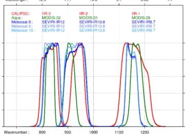
Figure 2. IIR/CALIPSO (red), MODIS/Aqua (green), and SE-VIRI/Meteosat 8, 9, 10 (navy blue, medium blue, light blue) in-strument spectral response functions against wavelength in microns (top x axis) and wavenumber in cm−1(bottom x axis).
3.2.2 Atmospheric inputs: the TIGR dataset
The simulations have been conducted for the 2311 atmo-spheres of the TIGR climatological library (Chédin et al., 1985; Chevallier et al., 1998). The 2311 atmospheres are sorted into five air mass types according to their virtual tem-perature profiles (Achard, 1991; Chédin et al., 1994), which are namely (1) tropical, (2) mid-lat1 for temperate condi-tions, (3) mid-lat2 for cold temperate and summer polar con-ditions, (4) polar1 for very cold polar concon-ditions, and (5) po-lar2 for winter polar conditions. The tropical air mass type is composed of 872 atmospheres, mid-lat1 and mid-lat2 are composed of 388 and 354 atmospheres, respectively, and po-lar1 and polar2 are composed of 104 and 593 atmospheres, respectively.
3.2.3 Brightness temperatures simulations
The 4A model and the TIGR atmospheres input data have been used to simulate the brightness temperatures of IIR and of the candidate companion channels. Each of the five TIGR air mass types includes one individual simulation for each in-dividual atmosphere included in the air mass type (i.e., 872 simulations for the tropical type, 388 for mid-lat1, 354 for mid-lat2, 104 for polar1, and 593 for polar2). Each TIGR air mass type is then characterized through the mean BTD between IIR and MODIS or SEVIRI channels and associ-ated standard deviations derived from the individual simu-lations (hereafter “TIGR_BTD”). The simusimu-lations presented here have been obtained using the 2009 version of the 4A/OP model described above, which does not call into question the initial evaluations conducted before the 2006 launch.
The most suitable radiometric pairings of IIR–MODIS channels for our study are IIR1–MODIS29, IIR2–MODIS31,
and IIR3–MODIS32. Similarly, the most suitable IIR– SEVIRI pairs are IIR1–SEVIRI8.7, IIR2–SEVIRI10.8, and IIR3-SEVIRI12. Simulations were for SEVIRI/Meteosat 8, which was the primary satellite in June 2006, but our chan-nel selection remains unchanged for the more recent instru-ments. The ISRFs of these nine channels are plotted in Fig. 2. ISRFs of SEVIRI Meteosat 9 and 10 are also shown for vi-sual comparison with Meteosat 8. Brightness temperatures derived from the modeled radiances are computed using the relevant ISRF. As an indication, shown in Table 2 are the equivalent central wavenumbers and wavelengths that min-imize the differences between the true temperature and the temperature derived using the Planck function over a range of temperatures stretching from 200 K to 310 K. The cen-tral wavenumbers are relevant in the case of blackbody ra-diances expressed in W m−2sr−1cm, as in the output of the 4A model, whereas the central wavelengths are relevant in the case of radiances reported in W m−2sr−1µm−1, as in IIR and MODIS satellite observations. It is noted that the equiv-alent central wavelengths of IIR1, IIR2, and IIR3 are found to be 8.635, 10.644, and 12.096 µm, respectively.
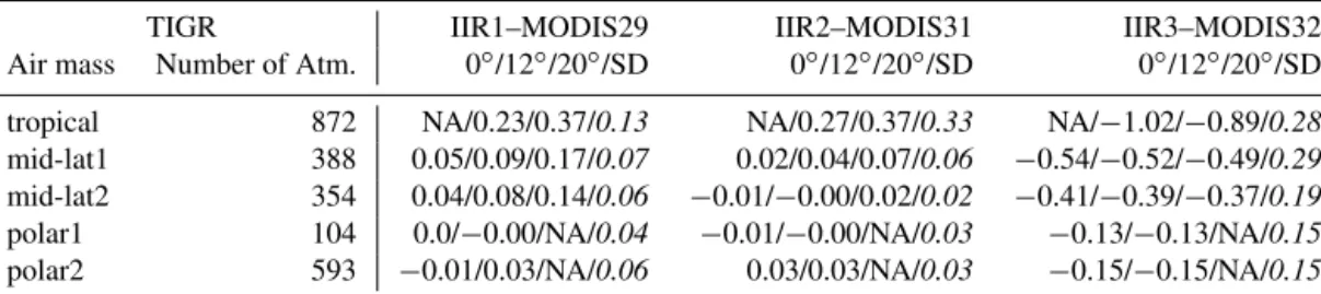
The TIGR_BTDs between IIR and MODIS companion channels are reported in Table 3 for the five TIGR air mass types. They are given for MODIS viewing angles of 0, 12, and 20◦, chosen according to the latitude-dependent, and therefore air mass type-dependent, range of viewing angles discussed in Sect. 3.1 and shown in Fig. 1. The TIGR_BTDs for each pair of companion channels and their variations with the TIGR air mass type encompass the difference in shape and position of the paired ISRFs and the inherent different sensitivity to surface temperature, temperature and water va-por profiles, and other absorbing atmospheric constituents. For the three pairs of channels, the absolute TIGR_BTDs and the standard deviations are overall larger for the tropi-cal air mass type than for the other air mass types, which is related to the high content and high variability of the water vapor in the tropical regions. Except for the tropics, abso-lute TIGR_BTDs are smaller than 0.2 K for IIR1–MODIS29 and 0.1 K for IIR2–MODIS31, with similar standard devi-ations smaller than 0.1 K. The largest absolute TIGR_BTDs and standard deviations are for the IIR3–MODIS32 pair, with TIGR_BTDs of about −1 K and standard deviations up to 0.3 K for tropical air mass types.
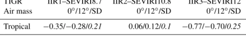
TIGR_BTDs between IIR and SEVIRI/Meteosat 8 com-panion channels for the TIGR tropical air mass and SEVIRI viewing angles equal to 0 and 12◦ are reported in Table 4. For a 12◦viewing angle, IIR–SEVIRI TIGR_BTDs differ by
up to 0.5 K from the respective IIR–MODIS TIGR_BTDs.
4 Implementation of the relative and stand-alone approaches
For both the relative and the stand-alone approaches, obser-vations of IIR and its companion channels are first spatially
Table 2. Equivalent central wavelengths and wavenumbers.
Channel/wavelength/ Channel/wavelength/ Channel/wavelength/ wavenumber wavenumber wavenumber IIR #1: 8.635 µm #2: 10.644 µm #3: 12.096 µm 1158.4 cm−1 939.9 cm−1 829.1 cm−1 MODIS #29: 8.553 µm #31:11.025 µm #32: 12.044 µm Aqua 1169.3 cm−1 907.6 cm−1 830.8 cm−1
SEVIRI IR8.7 IR10.8 IR12
Meteosat 8 1148.7 cm−1 929.3 cm−1 838.7 cm−1 Meteosat 9 1148.2 cm−1 930.1 cm−1 835.8 cm−1 Meteosat 10 1147.7 cm−1 928.7 cm−1 838.0 cm−1
Table 3. Simulated brightness temperature difference (TIGR_BTD) in Kelvin between IIR and MODIS/Aqua companion channels for MODIS viewing angles of 0, 12, and 20◦, whenever relevant (NA if not), and standard deviation (in italic) for five air mass types from the TIGR data base.
TIGR IIR1–MODIS29 IIR2–MODIS31 IIR3–MODIS32 Air mass Number of Atm. 0◦/12◦/20◦/SD 0◦/12◦/20◦/SD 0◦/12◦/20◦/SD tropical 872 NA/0.23/0.37/0.13 NA/0.27/0.37/0.33 NA/−1.02/−0.89/0.28 mid-lat1 388 0.05/0.09/0.17/0.07 0.02/0.04/0.07/0.06 −0.54/−0.52/−0.49/0.29 mid-lat2 354 0.04/0.08/0.14/0.06 −0.01/−0.00/0.02/0.02 −0.41/−0.39/−0.37/0.19 polar1 104 0.0/−0.00/NA/0.04 −0.01/−0.00/NA/0.03 −0.13/−0.13/NA/0.15 polar2 593 −0.01/0.03/NA/0.06 0.03/0.03/NA/0.03 −0.15/−0.15/NA/0.15
and temporally collocated, as described below, followed by the various steps specific to the implementation of each ap-proach.
4.1 Collocations
Collocated observations are from the REMAP product that is developed, processed, and available at the AERIS/ICARE data center. REMAP includes MODIS/Aqua and SEVIRI calibrated radiances collocated with the IIR Level 1B radi-ances and remapped onto the IIR 69 km grid. MODIS cal-ibrated radiances are from MYD021KM Collection 5 (C5) with geolocation from MYD03 C5. SEVIRI geolocated and calibrated radiances are from the Level 1.5 Image product, which reports spectral blackbody radiances until 7 May 2008 and effective blackbody radiances afterwards (EUMETSAT, 2007b). For each IIR pixel, the collocated MODIS or SE-VIRI radiance is from the closest pixel, at sea level. So far, no spatial averaging of the IIR or MODIS 1 km pixels is per-formed in order to get a better match with SEVIRI pixels. Thus, one 3 km resolution sub-satellite SEVIRI pixel is col-located with at least nine different IIR pixels, depending on the SEVIRI viewing angle. IIR and MODIS pixels are col-located with the temporally closest SEVIRI image, which is up to 7 min 30 s before or after the companion observation. IIR and MODIS observations are quasi-coincident and are therefore considered always temporally collocated. Overall,
IIR and MODIS observations are well collocated, whereas a naturally occurring GEO–LEO “mismatch” between SEVIRI and IIR observations cannot be ignored spatially, because of the difference in the pixel sizes and the difference in the satel-lite zenith angles, nor ignored temporally, because the time difference between the observations can be up to several min-utes. This spatial mismatch is minimized by comparing IIR and SEVIRI when SEVIRI viewing angles are less than 10◦.
4.2 Relative approach: outputs and statistical analyses
Outputs of the relative approach are presented here show-ing daily means of BTDs and standard deviations. They have been generated for each single day since launch, with day-time and nightday-time data either combined or separated, for several 10 K ranges of observed brightness temperatures, from 290–300 down to 200–210 K.
Statistical analyses of BTDs between pairs of channels over ocean are performed for five latitude ranges: in the tropics (30◦S–30◦N), and at mid- (30–60◦) and polar (60–
82◦) latitudes in both hemispheres. Oceanic scenes are iden-tified using an index available from the Global Land One-kilometer Base Elevation (GLOBE) project (GLOBE Task Team and others, 1999). Thresholds are defined, which are based on the simulated TIGR_BTDs and associated standard deviations (see Tables 3 and 4) and on the ex-pected instrumental NedT (see Table 1). A “worst case”
Table 4. Simulated brightness temperature difference (TIGR_BTD) in Kelvin between IIR and SEVIRI/Meteosat 8 companion channels for SEVIRI viewing angles of 0 and 12◦, and standard deviation (in italic) for the tropical air mass type from the TIGR data base.
TIGR IIR1–SEVIRI8.7 IIR2–SEVIRI10.8 IIR3–SEVIRI12 Air mass 0◦/12◦/SD 0◦/12◦/SD 0◦/12◦/SD Tropical −0.35/−0.28/0.21 0.06/0.12/0.1 −0.77/−0.70/0.25
standard deviation σ has been computed by taking 0.4 K for TIGR_BTD, the IIR NedT specified before launch (0.5 K), and NedT = 0.1 K for MODIS and SEVIRI, yield-ing σ = 0.7 K. Usyield-ing TIGR_BTDs correspondyield-ing to each lat-itude band, BTDs larger or smaller than TIGR_BTD ± 3σ (i.e., ±2.1 K) are considered unrealistic values due to the fact that the instruments presumably do not see the same scenes. The statistics are computed after rejecting these unre-alistic values. Because the collocations are at sea level, these tests should minimize parallax issues in the case of elevated clouds.
4.3 Stand-alone approach 4.3.1 Clear sky mask
After collocation of IIR, MODIS, and SEVIRI companion channels (Sect. 4.1), a clear sky mask is applied to select the relevant pixels for direct comparisons between observations and simulations. The mask is from the Version 3 IIR Level 2 swath product (Vaughan et al., 2015). It is derived from col-located IIR and CALIOP observations along the lidar track and extended to the 69 km IIR swath by using radiative ho-mogeneity criteria (Garnier et al., 2012). In the Version 3 IIR Level 2 operational algorithm, clear sky track pixels are fined as those pixels for which no cloud layers could be de-tected by CALIOP and no depolarizing aerosol layers could be detected after averaging the lidar signal up to 20 km along the track. This information is extracted from the CALIOP Level 2 5 km cloud and aerosol layer products (Vaughan et al., 2015). Initial analyses determined that the Version 3 mask is contaminated by the presence of low cloud layers detected by CALIOP at the finest 1/3 km resolution, but not reported in the 5 km layer product, so they are ignored by the IIR algorithm. This issue will be corrected in the next version (4) of the IIR operational algorithm. Because the new opera-tional product is not available at this time, a corrected mask has been produced specifically for this study. We chose to process each occurrence of January and July from mid-June 2006 to December 2015 to cover the same 9.5-year time pe-riod as used in the relative approach for two opposite seasons. 4.3.2 Clear sky brightness temperatures simulations Clear sky simulations of the collocated observations (Sect. 4.1) are carried out using the 4A/OP model (see Sect. 3.2.1) and the temporally and spatially closest
atmo-spheric profiles and ocean skin temperatures given by ERA-Interim (ERA-I) reanalyses generated at the European Centre for Medium-Range Weather Forecast (ECMWF). We have chosen to use outputs from reanalyses over outputs based on radiosondes measurements (e.g., the LMD Analyzed Ra-dioSoundings Archive, ARSA, database) because of the low density of the radiosonde network over sea. ERA-I reanaly-ses are available every 6 h with a nominal resolution of 0.75◦ in latitude and longitude. The 4A/OP-simulated radiances are computed for each clear pixel found at a distance smaller than 5 km from the closest ERA-I input to ensure the high-est possible coherence for the comparisons with the observa-tions. This 5 km threshold was chosen by taking into account the specificity of each of the three instruments (IIR, MODIS, and SEVIRI). The reanalyses outputs give a 61-level descrip-tion of the temperature, water vapor, and ozone profiles as well as the skin temperature. A comprehensive documen-tation of the current ERA-I reanalysis system used in this study may be found in Dee et al. (2011). For other absorbers with a constant pressure-dependent mixing ratio (CO2, N2O,
CO, HNO3, SO2, CFCs, etc.), the most plausible mixing ratio
value is used.
The MODIS and SEVIRI viewing angles are outputs of the collocation step (Sect. 4.1), and the IIR is considered a nadir viewing instrument.
Another essential variable for the simulation of the bright-ness temperatures of these nine window channels is the ocean surface emissivity. As shown for a long time, in many pub-lications, the emissivity depends on wind speed, polariza-tion, temperature, emission angle, and wavenumber (Ma-suda et al., 1988; Wu and Smith, 1996; Brown and Minnett, 1999; Hanafin and Minnett, 2005; Niclòs et al., 2007). In the present study, variations with wind speed or polarization are not taken into account. Indeed, we chose to favor the consis-tency with the prelaunch simulations so ocean surface emis-sivity has been set to 0.98 for all the channels. Again, be-cause MODIS viewing angles are always smaller than 20◦ and SEVIRI-selected angles are intentionally limited to 10◦, the emissivity dependence on satellite viewing angles is ne-glected. It is worth pointing out that problems requiring the highest possible absolute accuracy, such as the retrieval of geophysical variables or the validation of radiative transfer models, could not be approached with such approximations. Here, we are more interested in comparing the behavior of the companion channels for each pair of channels than in comparing the pairs. Because each companion channel of
each pair is processed under the same conditions, using this constant value of the emissivity, there would be a negligible effect on their relative behavior. However, in the planned fu-ture reprocessing of the data, and since no limitation comes from the 4A/OP model itself, the required dependencies will be taken into account, in detail, whenever the information is available.
4.3.3 Outputs and statistical analyses
The stand-alone approach generates, for each channel, differ-ences between the 4A simulation and the clear sky observa-tion, hereafter called “residuals”. For this study, the 4A sim-ulations have been processed for 10 days of each of the cho-sen months. Outputs are “monthly” mean residuals and asso-ciated standard deviations, with daytime and nighttime data either combined or separated. Statistics are built monthly in-stead of daily, as done in the relative approach, because the number of samples is smaller due to the severe collocation constraints described above. Final statistics are given after re-moving individual residuals found outside the initial monthly mean ± twice the initial standard deviation. This procedure is done to prevent undetected cloudy pixels to enter the statis-tics as well as for situations for which the instruments pre-sumably do not see the same scenes.
5 Results and findings from the relative approach Results from the relative approach are presented hereafter in terms of time series of daily averaged (day and night com-bined) IIR–MODIS and IIR–SEVIRI BTDs between mid-June 2006 and the end of December 2015. The findings de-rived from the analysis of the various figures are then dis-cussed.
5.1 Results
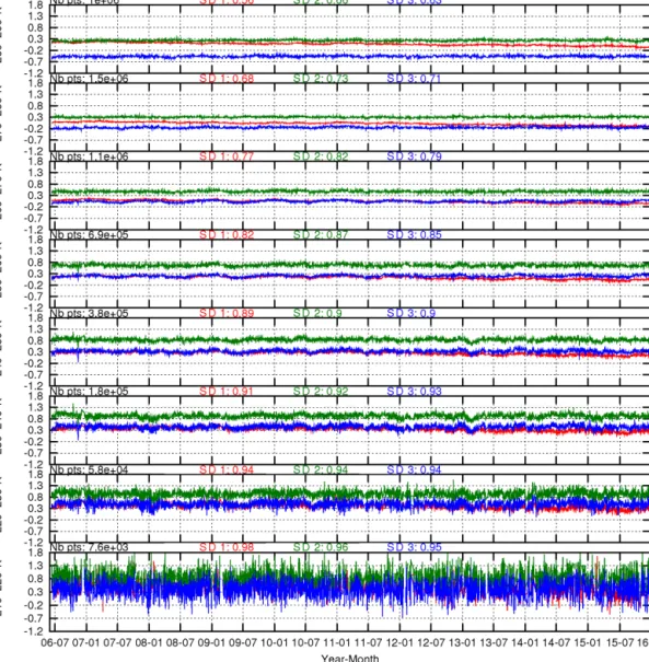
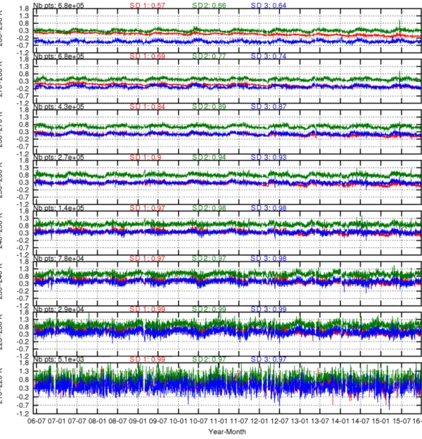
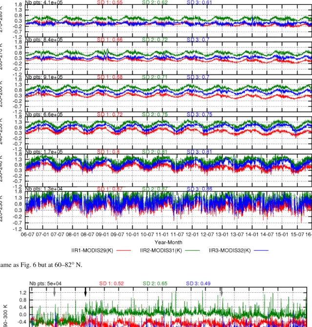
Time series of IIR–MODIS BTD are shown in Figs. 3 to 7 for the five latitude bands, namely 30◦S–30◦N (Fig. 3), 60– 30◦S (Fig. 4), 30–60◦N (Fig. 5), 82–60◦S (Fig. 6), and 60– 82◦N (Fig. 7). Each of these figures includes several pan-els corresponding to 10 K brightness temperature domains (decreasing from top to bottom) typically found in their re-spective latitude bands, and each panel shows the BTD for the three pairs of channels: IIR1–MODIS29 (red), IIR2– MODIS31 (green), and IIR3–MODIS32 (blue). The mean number of pixels per day used to build the statistics and the mean standard deviations for each pair of channels are shown at the top of each panel and also in Table 5 for more clar-ity. The mean number of daily pixels is always larger than 5 × 10³and up to 3.7 × 10⁶in the tropics at 290–300 K. For each latitude band, the smallest standard deviations are found at the warmest temperatures, with standard deviations rang-ing from 0.44 to 0.66 K. Standard deviations increase up to 1.1 K in the tropics at the coldest temperatures, generally
as-sociated with increased instrument noise, but perhaps also due in part to larger inhomogeneity of cloudy scenes and to parallax effects at larger MODIS viewing angles. The large daily variability seen at mid- and high latitudes at the coldest temperatures is also attributed to the smaller number of sam-ples (see Table 5). Overall, the results show very stable IIR– MODIS BTD since the CALIPSO launch, with some sea-sonal variations noted, but with a remarkable year-by-year repeatability. These features will be discussed in more detail in Sect. 5.2. It is confirmed that the switch from 0.3 to 3◦ of the CALIPSO platform pitch angle at the end of Novem-ber 2007 (see Sect. 2) has no significant impact, because no discontinuity in the time series can be evidenced.
Time series of IIR–SEVIRI BTD are shown in Fig. 8 for comparison with the IIR–MODIS time series. As explained in Sect. 3.1, only SEVIRI viewing angles smaller than 10◦ are chosen. Consequently, the comparisons are only between about 10◦W and 10◦E in longitude and between 10◦S and
10◦N in latitude. The temperature range is 290–300 K. The mean number of samples per day (5 × 10⁴) is about 100 times smaller than for the IIR–MODIS comparisons. More-over, the day-to-day variability is more important and the standard deviations are slightly larger (between 0.49 and 0.65 K). The black and grey arrows point to discontinuities in the time series. The discontinuity of up to 0.4 K in May 2008 (black arrows) is explained by the change of definition in the SEVIRI 1.5 image product from spectral to effective black-body radiances on 7 May 2008. For simplicity, this change is not accounted for in this analysis, which assumes effec-tive blackbody radiances. This discontinuity was already ev-idenced in the initial analyses reported in Scott (2009). In addition, discontinuities of smaller amplitude (grey arrows) are seen in April 2007, which correspond to the switch from Meteosat 8 to Meteosat 9, and in January 2013, which co-incide with the switch to Meteosat 10. These small disconti-nuities are explained by the fact that the SEVIRI brightness temperatures are computed using the Meteosat 8 ISRFs for the entire period. The discontinuities in the time series illus-trate the sensitivity of the technique to detect instrumental changes.
5.2 Findings
As seen in Sect. 5.1, considering the fact that the IIR and MODIS/Aqua both fly in the A-Train, and considering no instrumental changes since CALIPSO launched, monitor-ing differences between IIR and MODIS/Aqua observations turns out to be a more fruitful approach for the assessment of the IIR calibration stability than monitoring differences between IIR and SEVIRI. Thus, the findings discussed in the following sections are based mostly on the IIR–MODIS com-parisons shown in Figs. 3 to 7. In this section, we discuss first the consistency of the IIR–MODIS and IIR–SEVIRI BTD at warm temperatures with our prelaunch evaluation from the five TIGR air mass types. Then, we successively discuss
Table 5. Mean number of pixels per day (bold) and mean standard deviations in Kelvin (from left to right: x = IIR1–MODIS29, y = IIR2– MODIS31, and z = IIR3–MODIS32) associated with Figs. 3 to 7.
30◦S–30◦N 60–30◦S 30–60◦N 82–60◦S 60–82◦N (Fig. 3) (Fig. 4) (Fig. 5) (Fig. 6) (Fig. 7) Pixels Pixels Pixels Pixels Pixels
x/y/z x/y/z x/y/z x/y/z x/y/z
290–300 K 3.7 × 10⁶ – – – – 0.48/0.63/0.48 280–290 K 2.1 × 10⁶ 1 × 10⁶ 6.8 × 10⁵ – – 0.83/0.88/0.84 0.56/0.66/0.63 0.57/0.66/0.64 270–280 K 5.4 × 10⁵ 1.5 × 10⁶ 6.8 × 10⁵ 5.9 × 10⁴ 4.1 × 10⁵ 0.87/0.95/0.94 0.68/0.73/0.71 0.69/0.77/0.74 0.44/0.52/0.5 0.55/0.62/0.61 260–270 K 1.7 × 10⁵ 1.1 × 10⁶ 4.3 × 10⁵ 6.0 × 10⁵ 8.4 × 10⁵ 1.1/1.1/1.1 0.77/0.82/0.79 0.84/0.89/0.87 0.61/0.68/0.64 0.66/0.72/0.70 250–260 K 1.1 × 10⁵ 6.9 × 10⁵ 2.7 × 10⁵ 1.0 × 10⁶ 9.1 × 10⁵ 1.1/1.1/1.1 0.82/0.87/0.85 0.90/0.94/0.93 0.61/0.67/0.63 0.68/0.71/0.70 240–250 K 7.9 × 10⁴ 3.8 × 10⁵ 1.4 × 10⁵ 8.1 × 10⁵ 6.6 × 10⁵ 1.1/1.1/1.2 0.89/0.90/0.90 0.97/0.98/0.98 0.62/0.69/0.65 0.72/0.75/0.75 230–240 K 6.6 × 10⁴ 1.8 × 10⁵ 7.8 × 10⁴ 2.6 × 10⁵ 1.7 × 10⁵ 1.1/1.1/1.2 0.91/0.92/0.93 0.97/0.98/0.98 0.65/0.72/0.71 0.80/0.81/0.81 220–230 K 5.7 × 10⁴ 5.8 × 10⁴ 2.9 × 10⁴ 9.8 × 10⁴ 1.3 × 10⁴ 1.1/1.1/1.1 0.94/0.94/0.94 0.99/0.99/0.99 0.67/0.71/0.71 0.87/0.87/0.86 210–220 K 3.9 × 10⁴ 7.6 × 10³ 5.1x × 103 – – 1.1/1.1/1.1 0.98/0.96/0.95 0.99/0.97/0.97 200–210 K 1.7 × 10⁴ – – – – 1.1/1.1/1.1
Table 6. IIR–MODIS brightness temperature differences in Kelvin at the beginning of the CALIPSO mission and associated uncertainty at the warmest temperature range in each latitude band.
Latitudes and temperatures IIR1–MODIS29 IIR2–MODIS31 IIR3–MODIS32 30◦S–30◦N, 290–300 K 0.336 ± 0.001 0.511 ± 0.002 −0.736 ± 0.001 60–30◦S, 280–290 K 0.176 ± 0.001 0.228 ± 0.001 –0.469 ± 0.001 30–60◦N, 280–290 K 0.170 ± 0.002 0.304 ± 0.003 −0.445 ± 0.003 82–60◦S, 270–280 K 0.121 ± 0.002 0.255 ± 0.002 −0.113 ± 0.002 60–82◦N, 270–280 K 0.159 ± 0.003 0.484 ± 0.004 0.055 ± 0.003
the IIR–MODIS results at cold temperatures, the long-term trends, and the seasonal variations.
5.2.1 Warm scenes
The first step of the analysis is to compare the mean BTD from the relative approach with the simulated TIGR_BTDs (see Sect. 3.2.3). Because the TIGR simulations are for clear sky conditions, the comparisons are conducted for the warmest temperature range at each latitude band. Indeed, the clear sky scenes are a priori the warmest ones, although the warmest scenes could also contain clouds of weak ab-sorption or thicker clouds located near the surface. After ap-plication of the (TIGR_BTD ± 2.1 K) thresholds introduced in Sect. 4.2, more than 95 % of the pixels contribute to the statistics, and the mean BTDs are changed by less than
0.15 K, confirming that the thresholding method is appropri-ate. The IIR–MODIS BTDs at the beginning of the mission derived from linear regression lines are reported in Table 6 for comparison against the TIGR_BTDs reported in Table 3. The observed IIR–MODIS BTDs in the tropics at 290–300 K and the TIGR_BTDs for tropical air mass types differ by less than 0.1 K for IIR1–MODIS29, 0.25 K for IIR2–MODIS31, and 0.3 K for IIR3–MODIS32. The observed mean BTD at 30–60◦ and at 280–290 K in the Northern and South-ern Hemispheres and the TIGR_BTDs at mid-latitude (mid-lat1 and mid-lat2) also agree within about 0.1 K for IIR1– MODIS29 and IIR3–MODIS32 and are within 0.2 to 0.3K for IIR2–MODIS31. The same conclusions apply for the mean BTD at 60–82◦S and at 270–280 K when compared
with the TIGR_BTDs for polar1 and polar2 atmospheres. At 60–82◦N, IIR2–MODIS31 and IIR3–MODIS32 BTDs
Figure 3. Time series (x axis: year-month) of daily averaged (day and night combined) IIR–MODIS brightness temperature differences (y-axis units: Kelvin) for the three pairs of companion channels (red: IIR1–MODIS29, green: IIR2–MODIS31, blue: IIR3–MODIS32) over ocean in the tropics at 30◦S–30◦N. Each panel is for a given range in brightness temperature from 290–300 K (top) down to 200–210 K (bottom). Added at the top of each panel are the mean number of points per day (Nb pts) and the mean standard deviation per day for each of the three pairs (see Table 5).
are larger than at 60–82◦S by about 0.2 K, which degrades the comparisons against the TIGR_BTDs. Overall, these re-sults demonstrate good consistency between observed IIR– MODIS BTDs and simulated TIGR_BTDs. Direct compar-isons between observations and simulations in clear sky
con-ditions will be discussed in Sect. 6 with the stand-alone ap-proach.
Even though the following is based on comparisons with MODIS/Aqua, it is interesting to compare the observed IIR– SEVIRI BTDs and the TIGR_BTDs in the tropics (Table 4).
Figure 4. Time series (x axis: year-month) of daily averaged (day and night combined) IIR–MODIS brightness temperature differences (y-axis units: Kelvin) for the three pairs of companion channels (red: IIR1–MODIS29, green: IIR2–MODIS31, blue: IIR3–MODIS32) over ocean at 60–30◦S. Each panel is for a given range in brightness temperature from 280–290 K (top) down to 210–220 K (bottom). Added at the top of each panel are the mean number of points per day (Nb pts) and the mean standard deviation per day for each of the three pairs (see Table 5).
After May 2008, when the radiances reported in the SEVIRI products are effective blackbody radiances, the TIGR_BTDs are in fair agreement with the differences plotted in Fig. 8, keeping in mind that the SEVIRI observations are from Me-teosat 9 and 10 after May 2008, whereas the TIGR simula-tions are for SEVIRI/Meteosat 8.
5.2.2 Cold scenes
As the scene temperature decreases, the clouds are denser and colder, and the contribution from such absorbing clouds increases while the influence of the surface and near-surface atmosphere decreases. The fraction of pixels retained after
application of the thresholding scheme described in Sect. 4.2 is found to decrease progressively from 95 % for the warm scenes to 30 %, with the smallest fraction observed at 200– 210 K in the tropics for the IIR3–MODIS32 pair. This is partly due to the fact that the BTDs are distributed over a broader range of values than anticipated, so that the mean BTD seen in Figs. 3 to 7 may be significantly, but system-atically, biased for the cold scenes. For a better quantifica-tion as temperature decreases, IIR–MODIS BTDs are evalu-ated using the median values of the whole distributions, with-out thresholding. The median value is preferred to the mean value to minimize the impact of presumably unrealistic val-ues. Median IIR1–MODIS29 (red), IIR2–MODIS31 (green),
Figure 5. Same as Fig. 4 but at 30–60◦N.
and IIR3–MODIS32 (blue) BTDs are shown in Fig. 9a by temperature ranges from 190–200 to 280–290 K in the trop-ics during 2008 for representative months of the four sea-sons. Mean absolute deviations from the median value are between 2.5 and 5 K. For further evaluation, IIR and MODIS inter-channel BTDs have been analyzed. Following the same approach as in Fig. 9a, Fig. 9b shows median IIR1–IIR3 (red, solid), IIR2–IIR3 (green, solid), MODIS29–MODIS32 (red, dashed), and MODIS31–MODIS32 (green, dashed) BTDs. Mean absolute deviations from the median value are be-tween 0.5 and 3 K. The variations of both IIR and MODIS inter-channel BTDs with temperature are due to the chang-ing optical and microphysical properties of absorbchang-ing ice and water clouds located at various altitudes. The analy-sis of arches as seen in Fig. 9b is the essence of the well-known split-window technique for the retrieval of cloud mi-crophysical properties (Inoue, 1985; Ackerman et al., 1990).
IIR and MODIS arches are not of the same amplitude be-cause IIR and MODIS measurements are spectrally differ-ent. The BTDs at the coldest temperatures (190–200 K) pro-vide useful information regarding the calibration. Indeed, the coldest temperatures (190–200 K) correspond a priori to ele-vated dense ice clouds, which, if they behave as blackbody sources, should lead to quasi-identical brightness temper-atures for all channels, assuming a negligible contribution from the atmosphere above the cloud. This is what we ob-serve in Fig. 9b, where the IIR and MODIS inter-channel BTDs are close to zero, showing internal consistency of the calibration within each instrument. However, Fig. 9a shows that the IIR–MODIS BTDs are about 1.6 K on average at 190–200 K for the three pairs of channels. This indicates a warm bias of 1.6 K of IIR with respect to MODIS at 190– 200 K. According to Fig. 9a, the warm bias seems to increase progressively as temperature decreases. An increasing IIR
Figure 6. Time series (x axis: year-month) of daily averaged (day and night combined) IIR–MODIS brightness temperature differences (y-axis units: Kelvin) for the three pairs of companion channels (red: IIR1–MODIS29, green: IIR2–MODIS31, blue: IIR3–MODIS32) over ocean at 82–60◦S. Each panel is for a given range in brightness temperature from 270–280 K (top) down to 220–230 K (bottom). Added at the top of each panel are the mean number of points per day (Nb pts) and the mean standard deviation per day for each of the three pairs (see Table 5).
calibration bias as temperature decreases could be explained by a drift of the gain with respect to the gain measured in flight at warm temperature. Because IIR has only one sensor, observing such a similar bias for all three channels is con-ceivable.
5.2.3 Long-term trends
IIR–MODIS BTDs are very stable year-by-year since mid-June 2006. In order to quantify the trends over the first 9.5 years of the CALIPSO mission, linear regression lines have been computed for each of the time series shown in Figs. 3 to 7. The slopes of these lines well approximate the trend of the IIR–MODIS brightness temperature differ-ences since the beginning of the CALIPSO mission. These trends are plotted against temperature in Fig. 10 for each pair of channels and for each of the five latitude bands. An unambiguous trend is seen for IIR1–MODIS29 (red) at any temperature and at any latitude, varying between −0.01 and
−0.03 K yr−1. It is −0.019 ± 0.0002 K yr−1 at 290–300 K in the tropics and −0.02 ± 0.0004 K yr−1 on average. This trend, which represents −0.19 K over the 9.5-year period, can also be seen directly in Figs. 3 to 7. However, the trend of the order of 0.005 K yr−1or less in absolute value for IIR2– MODIS31 (green) and IIR3–MODIS32 (blue) is deemed not significant. Notwithstanding the small trend evidenced for IIR1–MODIS29, which is further investigated in Sect. 6 us-ing the stand-alone approach, the long-term stability of the IIR instrument with respect to MODIS/Aqua between June 2006 and the end of 2015 is remarkable.
5.2.4 Seasonal variations
Seasonal variations of the IIR–MODIS BTD are sometimes observed at mid- and high latitude in Figs. 4 to 7. More specifically, it can be noted by comparing Figs. 4 and 5 on one hand (mid-latitudes) and Figs. 6 and 7 on the other hand (polar latitudes) that at any scene temperature, including the
Figure 7. Same as Fig. 6 but at 60–82◦N.
Figure 8. Time series (x axis: year-month) of IIR–SEVIRI brightness temperature differences (y-axis units: Kelvin) for the three pairs of companion channels (red: IIR1–SEVIRI8.7, green: IIR2–SEVIRI10.8, blue: IIR3–SEVIRI12) over ocean at 290–300 K for SEVIRI viewing angles smaller than 10◦. Added at the top of each panel are the mean number of points per day (Nb pts) and the mean standard deviation per day for each of the three pairs. The black arrows indicate the change in the definition of the SEVIRI product in May 2008. The grey arrows indicate the switch from Meteosat 8 to 9 in April 2007 and from Meteosat 9 to 10 in January 2013.
warmest temperatures, with presumably the smallest influ-ence from clouds, a seasonal variability is clearly seen in the Northern Hemisphere but barely in the Southern Hemi-sphere. It was found that at mid-latitudes, where observations during both daytime and nighttime are available year-round,
the larger seasonal variability in the Northern Hemisphere is related to significant differences between nighttime and daytime IIR–MODIS BTDs. This is illustrated in Figs. 11 and 12, where the IIR–MODIS BTDs are shown for each pair of channels at 30–60◦N (Fig. 11) and at 60–30◦S (Fig. 12),
Figure 9. (a) Median IIR1–MODIS29 (red), IIR2–MODIS31 (green), and IIR3–MODIS32 (blue) brightness temperature differences against brightness temperature. (b) Median IIR1–IIR3 (red, solid), IIR2–IIR3 (green, solid), MODIS29–MODIS32 (red, dashed), and MODIS31– MODIS32 (green, dashed) brightness temperature differences against temperature. Plus sign: January 2008, star: April 2008, diamond: July 2008, triangle: October 2008. Latitude band: 30◦S–30◦N, ocean.
Figure 10. Trends of IIR–MODIS brightness temperature differences and associated uncertainties against temperature for the three pairs of companion channels (red: IIR1–MODIS29, green: IIR2–MODIS31, blue: IIR3–MODIS32) as derived from Figs. 3 to 7. Latitude bands: diamond, 30◦S–30◦N; square, 60–30◦S; circle, 30–60◦N; inverse triangle, 82–60◦S; triangle, 60–82◦N.
at 280–290 K, and by distinguishing daytime data (in red) from nighttime data (in blue). The BTDs obtained by com-bining daytime and nighttime data, as in Figs. 4 and 5, are plotted in black for reference. At 30–60◦N (Fig. 11), sea-sonal night/day biases are seen for the three pairs of IIR– MODIS channels, whereas no night/day biases are seen in the Southern Hemisphere at 60–30◦S (Fig. 12). The largest bias at 30–60◦N is during June and July, with a night-minus-day difference equal to +0.4 K for IIR2–MODIS31 (middle) and IIR3–MODIS32 (bottom) and equal to about +0.2 K for IIR1–MODIS29 (top). In the opposite season, no night/day bias is seen for IIR1–MODIS29, whereas the night–day dif-ference is about −0.1 K for the other pairs. This behavior is further discussed in Sect. 6 after the presentation of addi-tional information from the stand-alone approach.
6 Results and further findings from the stand-alone approach
The stand-alone approach has been applied to each of the three IIR channels and each of their three MODIS and SE-VIRI companion channels to directly compare clear sky sim-ulations and clear sky measurements. Here, results are shown for IIR and MODIS only, for each month of January and July from mid-2006 to the end 2015, with the corrected clear sky mask processed as described in Sect. 4.3.1. From the relative approach (Sect. 5.2.3), a trend of −0.02 K yr−1 on average is detected for IIR1–MODIS29, which could originate from one channel or from both. The stand-alone approach allows the asserting of which channel deviates from the other. Sim-ilarly, the night/day biases evidenced for each pair of
chan-Figure 11. Time series (x axis: year-month) of IIR–MODIS brightness temperature differences (y-axis units: Kelvin) for the three pairs of companion channels (a IIR1–MODIS29, b IIR2–MODIS31, c IIR3–MODIS32) over ocean at 30–60◦N and 280–290 K. Red: day only, blue: night only, black: day and night.
nels in the Northern Hemisphere at 30–60◦(Sect. 5.2.4) are investigated.
6.1 Results
The fraction of clear sky IIR pixels over ocean is the largest in the tropics at 30◦S–30◦N, with 20 % of the ocean pix-els on average at nighttime and 25 % daytime. The slightly larger daytime fraction could be in part due to the smaller signal to noise ratio of the lidar signal and therefore to a reduced ability to detect clouds. Figure 13 shows the mean monthly residuals obtained over ocean in the tropics for IIR1 and MODIS29 (top), IIR2 and MODIS31 (middle), and IIR3 and MODIS32 (bottom) night and day. Each monthly value is obtained from typically 4 × 10³simulations. Linear regres-sion lines with temporal origin at the beginning of the mis-sion are also plotted, with slopes and intercepts given on each panel. The residuals are found between 0.2 and 0.6 K, which is deemed reasonable, keeping in mind that they are sensi-tive to the auxiliary data (including the clear sky mask) and that the surface emissivity is made constant and equal to 0.98 for all channels. The standard deviations are found between 0.4 and 0.6 K for the IIR channels and between 0.5 and 0.7 K for the MODIS channels. Values from IIR and MODIS are comparable, showing the importance of uncertainties in an-cillary inputs as compared to the instrumental noise. Using the Version 3 non-corrected IIR clear sky mask leads to sig-nificantly larger standard deviations, up to 1.2 K. Moreover, these residuals are larger by about 0.5 K, with season- and latitude-dependent biases, which is fully consistent with the presence of unwanted clouds and therefore too-cold observa-tions in these supposedly clear sky data samples.
The IIR1 (0.412 K) and MODIS29 (0.392 K) residuals shown in Fig. 13 differ by only 0.02 K at the beginning of the mission, and IIR2 (0.208 K) and MODIS31 (0.249 K) residuals differ by only 0.04 K. This indicates that for these
pairs, the differences between the observations are well re-produced by the simulations, suggesting an excellent ac-curacy of the IIR calibration. However, the IIR3 residuals (0.324 K) are smaller than the MODIS32 residuals (0.579 K) by −0.26 K. Because residuals are differences between simu-lations and observations, this means that the simulated IIR3– MODIS32 differences are smaller than the observed differ-ences by −0.26 K.
6.2 Further findings 6.2.1 IIR1–MODIS29 trend
Similar temporal variations of the monthly residuals in Fig. 13, of the order of less than 0.1 K, are seen for all the channels of the two instruments, indicating that they orig-inate from the simulations rather than from the observa-tions. The slope of the MODIS29 residuals, −0.019 K yr−1, is much larger than that of IIR1, 0.0017 K yr−1, meaning that MODIS29 observations have increased with respect to the simulations at a rate of +0.019 K yr−1, whereas IIR1 ones have barely changed. This is in perfect agreement with the decrease of IIR1–MODIS29 BTD at a rate of −0.019 K yr−1 seen in the relative approach at 290–300 K in the tropics. For the IIR2–MODIS31 and IIR3–MODIS32 pairs, the ab-sence of a detectable trend in the relative approach suggests that none of these four channels has been drifting. As ex-pected, the slopes of the four residuals are quasi-identical and do not exceed −0.0037 K yr−1. Overall, this indicates that the much larger slope of the MODIS29 residuals is driven by MODIS observations and not by the simulations. In conclusion, none of the IIR channels exhibit a detectable trend, whereas MODIS29 exhibits a positive trend of about +0.019 K yr−1since the beginning of the CALIPSO mission. It is recalled that MODIS C5 products are used for this
anal-Figure 12. Same as Fig. 11, but at 60–30◦S.
Figure 13. Time series (x axis: year-month) of residuals (y-axis units: Kelvin) for the three pairs of IIR and MODIS channels (a IIR1 and MODIS29 in red, b IIR2 and MODIS31 in green, c IIR3 and MODIS32 in blue, with IIR in full circles and MODIS in open circles) over ocean in the tropics at 30◦S–30◦N, day and night. Superimposed are linear regressions lines with temporal origin at the beginning of the mission. Slopes (in K yr−1) and intercepts (in K) are given on each panel.
ysis, so this assessment may not be applicable to the most recent Collection 6 (C6).
6.2.2 IIR–MODIS night/day bias at 30–60◦N
A night/day bias has been evidenced for each pair of IIR– MODIS observations in the Northern Hemisphere at 30– 60◦, which varies seasonally and has its maximum ampli-tude in June and July (see Sect. 5.2.4 and Fig. 11). For
fur-ther assessment, Fig. 14 shows the IIR and MODIS resid-uals for the three pairs of channels against latitude for the month of July 2007 by separating nighttime (top) and day-time (bottom) clear sky observations. Again, the results have to be interpreted in a relative sense. At night (top) and south of 25◦N, the IIR1 and MODIS29 residuals (red curves) and the IIR3 and MODIS32 residuals (blue curves) exhibit quasi-identical latitudinal variations, which are therefore at-tributed to the simulations. IIR2 and MODIS31 residuals
Figure 14. Residuals against latitude in July 2007 for the three pairs of IIR and MODIS channels (IIR1 and MODIS29: red, IIR2 and MODIS31: green, IIR3 and MODIS32: blue, IIR: full circles, MODIS: open circles). (a) Night. (b) Day.
(green curves) are very close from 35◦S to 25◦N and slightly depart from each other by up to 0.2 K south of 35◦S. Sim-ilar results are obtained during daytime (bottom) south of 25◦N. At night, from 25 to 45◦N, the three MODIS resid-uals (open circles) and the IIR1 residresid-uals (red, full circle) have similar latitudinal variations, whereas IIR2 (green, full circle) and IIR3 (blue, full circle) residuals unambiguously decrease more rapidly than the others, by about 0.5 K. How-ever, during daytime, no distinct behavior of the IIR2 and IIR3 residuals is seen between 25 and 45◦N. The sudden
de-crease from 25 to 45◦N seen for the IIR2 (respectively IIR3) nighttime residual, but not for the residual of its compan-ion channel MODIS31 (respectively MODIS 32), indicates that this phenomenon originates from the observations. Fur-thermore, the fact that this sudden decrease is seen only for the IIR2 and IIR3 residuals and is seen at night but not dur-ing the day strongly suggests a calibration bias in IIR2 and IIR3 observations at night. A sudden decrease of the residu-als means a sudden increase of the IIR2 and IIR3 brightness temperatures, by up to 0.5 K from about 30 to 45◦N. Thus, the stand-alone approach shows that the night-minus-day differences of +0.4 K seen for IIR2–MODIS31 and IIR3– MODIS32 in June and July in the Northern Hemisphere at 30–60◦(Fig. 11) using the relative approach are due to the
fact that IIR2 and IIR3 channels are biased and too warm at night. It is recognized that the smaller night–day differences seen for IIR1–MODIS29 (+0.2 K) in Fig. 11 are not clearly evidenced from the stand-alone approach. No issue is evi-denced in the Southern Hemisphere and south of 25◦N from the stand-alone approach, which is consistent with the fact that nighttime and daytime IIR–MODIS BTDs at 60–30◦in the Southern Hemisphere are nearly identical (Fig. 12).
It is noted that south of 25◦N, all nighttime residuals tend to be larger than daytime ones, by about 0.2 K. However, dif-ferences due to the clear sky mask are expected to lead to larger daytime residuals because of the a priori larger proba-bility for the lidar to miss clouds during daytime. Thus, even though the clear sky mask may partly explain these differ-ences, it is likely not the only contributor. Nevertheless, these small differences do not impact the previous discussion.
The IIR calibration biases evidenced at mid-latitude in the Northern Hemisphere are being investigated in collaboration with CNES. Our current understanding is that the rapidly changing thermal environment of the instrument at the end of the daytime portion and at the beginning of the nighttime portion of the orbits in the Northern Hemisphere would not be perfectly accounted for through the blackbody source used for the in-flight calibration. The flaw is synchronized with the elapsed time since the night-to-day transition along the orbit. Because the latitude of the night-to-day transition depends on the season, the flaw appears at season-dependent latitudes but always in the Northern Hemisphere (T. Trémas, personal communication, 2012), which in turn explains the observed seasonal variations at fixed latitudes (30–60◦N). These cal-ibration biases are expected to impact the IIR1–IIR3 inter-channel BTD by less than 0.2 K on average and to have no significant impact on IIR2–IIR3 on average.
7 Summary and conclusions
An assessment of the IIR calibration after 9.5 years of nearly continuous operation has been presented. IIR channels IIR1 (8.65 µm), IIR2 (10.6 µm), and IIR3 (12.05 µm) have been primarily compared against MODIS/Aqua C5 compan-ion channels MODIS29, MODIS31, and MODIS32, respec-tively, both on the A-Train with no instrumental changes since the CALIPSO launch. The choice of the companion instruments and channels was based on criteria such as spec-tral range and BTD between IIR and the candidate chan-nels, quality and frequency of the spatial and temporal co-incidences with the IIR 69 km swath, and spatial resolution. The BTD between IIR and its companion channels had been evaluated before launch using the 4A radiative transfer model and five air mass types determined from the TIGR climatic data base (TIGR_BTD, Table 3). The simulation, colloca-tion, and statistical tools have also been developed to perform comparisons with SEVIRI companion channels SEVIRI8.7, SEVIRI10.8, and SEVIRI12.
Two complementary approaches have been applied, which aim at characterizing deviations between the pairs of com-panion channels as well as the behavior of each individual channel both qualitatively and quantitatively. The relative ap-proach is based on statistical analyses of BTD between IIR and the relevant companion channels in controlled condi-tions, over a wide range of brightness temperatures and over ocean. This approach uses only calibrated and geolocated