Climate Variability and Internal Migration: A Test on Indian Inter-State Migration
Texte intégral
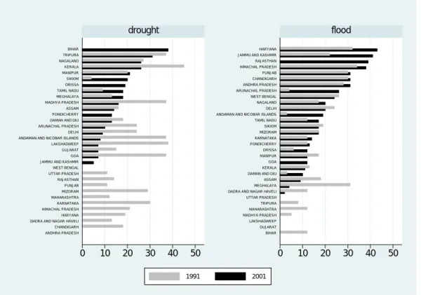
Figure
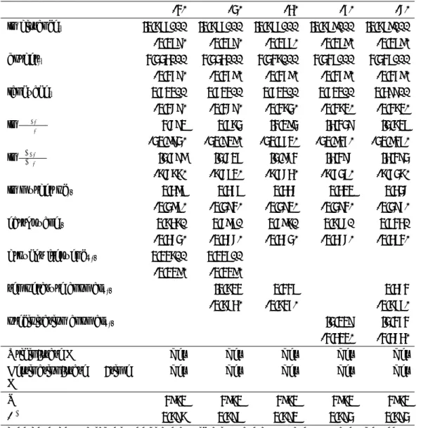
![Figure 1: Maps of India interstate out-migration by state, 1991 and 2001 (270000,360000] (120500,270000] (67000,120500] (42000,67000] (30500,42000] (3500,30500] (2000,3500] (1000,2000] [0,1000] No data1990-1991 2000-2001](https://thumb-eu.123doks.com/thumbv2/123doknet/13223975.394213/8.918.200.719.147.490/figure-maps-india-interstate-migration-state-data.webp)


Documents relatifs
In the Part Two we investigated the relative importance of strain, beak condition (trimmed or not trimmed) and rearing condition (access to litter from day one on or from four
L’archive ouverte pluridisciplinaire HAL, est destinée au dépôt et à la diffusion de documents scientifiques de niveau recherche, publiés ou non, émanant des
Climate variability of the last 2700 years in the Southern Adriatic Sea: Coccolithophore evidences.. Antonio Cascella, Sergio Bonomo, Bassem Jalali, Marie-Alexandrine Sicre,
APA errors were associated with a specific alpha/beta oscillation profile over the sensorimotor cortex; these beta oscillations might be sensitive markers of non-conscious
Alors, les pointés associées à une grande erreur pourraient être écartés ou pour le moins pondérés par de faible poids avant les traitements a posteriori des premières
Au-delà d’améliorer notre compréhension de la diversité, la biogéographie et l’écologie des Collodaires dans l’océan mondial, ce travail de thèse souligne
(D) Diffusive downward fluxes (integrated with the height of overlying water) of dissolved uranium in the different treatments estimated from concentration profiles. Different
In the past, migration that was essentially from rural to urban areas but also towards other rural areas, came from semi-arid regions (Middle Valley of the Senegal
