Publisher’s version / Version de l'éditeur:
Proceedings 18th International Conference on Port and Ocean Engineering under Arctic Conditions, 2, pp. 555-564, 2005
READ THESE TERMS AND CONDITIONS CAREFULLY BEFORE USING THIS WEBSITE. https://nrc-publications.canada.ca/eng/copyright
Vous avez des questions? Nous pouvons vous aider. Pour communiquer directement avec un auteur, consultez la
première page de la revue dans laquelle son article a été publié afin de trouver ses coordonnées. Si vous n’arrivez pas à les repérer, communiquez avec nous à [email protected].
Questions? Contact the NRC Publications Archive team at
[email protected]. If you wish to email the authors directly, please see the first page of the publication for their contact information.
Archives des publications du CNRC
This publication could be one of several versions: author’s original, accepted manuscript or the publisher’s version. / La version de cette publication peut être l’une des suivantes : la version prépublication de l’auteur, la version acceptée du manuscrit ou la version de l’éditeur.
Access and use of this website and the material on it are subject to the Terms and Conditions set forth at Iceberg shape characterization
McKenna, Richard
https://publications-cnrc.canada.ca/fra/droits
L’accès à ce site Web et l’utilisation de son contenu sont assujettis aux conditions présentées dans le site LISEZ CES CONDITIONS ATTENTIVEMENT AVANT D’UTILISER CE SITE WEB.
NRC Publications Record / Notice d'Archives des publications de CNRC:
https://nrc-publications.canada.ca/eng/view/object/?id=8db8d405-c450-4bb2-af15-196985fead02 https://publications-cnrc.canada.ca/fra/voir/objet/?id=8db8d405-c450-4bb2-af15-196985fead02
ICEBERG SHAPE CHARACTERIZATION
Richard McKenna Consultant
Wakefield, Québec, CANADA
ABSTRACT
The present iceberg shape characterization ties the above and below water portions of the iceberg in a consistent manner, satisfies hydrostatic considerations, represents measured relationships between waterline length, waterline width, height, draft and mass, and can be used for probabilistic simulations. The approach involves the characterization of three dimensional iceberg shape in terms of the overall average shape and a random component based on the concepts of spatial statistics. The approach has a predictive capability that provides for the generation of a large number of complete iceberg shapes, each with the statistical attributes of measured data.
The approach is illustrated through the analysis of two full iceberg profiles collected during the DIGS experiment conducted offshore Labrador in 1985. Many representative iceberg geometries were generated from the statistics of the DIGS icebergs, which were then reoriented and adjusted vertically in the water column to satisfy hydrostatic
considerations. Index dimensions were calculated from the generated shapes and their interrelationships were compared with those derived from measured data. The approach yielded realistic iceberg shapes and should be useful for generating iceberg shapes for assessment of risk to Grand Banks installations.
INTRODUCTION
Iceberg shape data are required to assess risk for a variety of installations off Canada’s east coast. Requirements include:
• determining the frequency of contact with fixed platforms, floating platforms and seabed installations;
• estimating the risk to topsides of production facilities;
• calculating the inertia of the iceberg relating to the point of impact; and • the development of the ice contact area on impact.
Although many field initiatives have been undertaken to document iceberg geometry, some inherent deficiencies become apparent when these data are used for the design of offshore installations. The deficiencies include gaps in the data due to difficulties with measurement near the water surface, a virtual absence of data from the base of the keels and many circumstances when only partial profile data are available.
There have been a few iceberg shape characterizations made in the past. The simplest is the MANICE designation (i.e. tabular, dome, drydock etc.), but this is not particularly useful for engineering analysis. More comprehensive formulations have included
relationships for contact area (e.g. Fuglem et al., 1998; McKenna et al., 2001), keel shape (e.g. PERD, 2000; Croasdale et al., 2001), and for overall shape (e.g. McKenna et al., 1999). Most of the above consider only a portion of the iceberg for specific purposes in the ice-structure interaction process. Those that treat the overall iceberg shape are simply representations of available data. The above have no real predictive capability, and they do not generally link above and below water portions of the iceberg. The present work, which addresses these issues, is a summary of PERD (2004a).
Data for full iceberg shape come primarily from field studies conducted in 1984 for the Hibernia project (Dobrocky Seatech, 1984), from isolated measurements such as the DIGS project (Hodgson et al., 1987) and from recent programs conducted by the Terra Nova project (PERD, 2004b). The DIGS data include underwater and above water information, and the present analysis includes two of these icebergs, for which horizontal contours were readily available in PERD (1999).
A STATISTICAL MODEL OF ICEBERG SHAPE Characterization of Deviations from the Mean
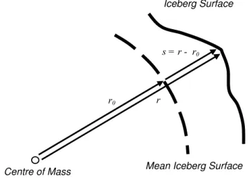
The surface points of the iceberg, ri, can be represented as the sum of the mean value, r0,
and a deviation, si, as shown in Figure 1. The mean shape is assumed to be spherical,
with radius r0. In vector form, this can be expressed as
(Eq.1) r = r0 + s
It is assumed that the deviation at each point on the surface of the iceberg can be represented as a linear combination of all the other deviations and a series of random values, ei. This can be expressed in the form
(Eq.2) s = B e
where B is a square matrix of coefficients, bi,j, relating surface points i and j (see Figure
2), and e is the vector of random values. Since E[r] = r0, the expected value of deviations, s, about the mean radius, r0, is
Iceberg Surface
s = r - r0
r r0
Figure 1 Deviation of a point on the iceberg surface from the mean shape
Figure 2 Geometry of the spherical mean iceberg shape
(Eq.3) E[s] = E[Be] = B E[e] = 0
so that E[e] = 0 as well.
The distribution of e can be ascertained from measured data. The first step is to solve for
r0, the next is to estimate B from the spatial correlations and the final one is to solve for
the random deviations from
(Eq.4) e = B-1(r - r0) = B-1 s
The spatial covariance of the deviations at the various surface points is (Eq.5) C = E[s sT] = E[B e (B e)T] = E[B e eT BT] = B E[e eT] BT
Mean Iceberg Surface Centre of Mass Z r0 X θ i φi Y αij (θi, φi) (θ j, φj) θj φj
since bi,j are constants and where E[ ] represents the expected value. The expression E[e eT] is simply I σe2, where σe2 is the variance of the random values, and C can be rewritten
(Eq.6) C = σe2 B BT
The covariance matrix, C, can also be expressed (Eq.7) C = σs2ρ
where σs2 is the variance and ρ is the correlation matrix of the deviations. Since there is
nothing constraining the magnitudes of B and e, the variances of the deviations s and e are chosen to be equal, i.e. σs2 = σe2 and the result is
(Eq.8) ρ = B BT
The coefficients of the matrix B can be solved from ρ using Cholesky factorization for positive definite forms and using a generalized matrix square root otherwise.
Spherical Geometry
The spherical mean shape with radius r0 is illustrated in Figure 2. Two surface points
with indices i, j are shown, along with corresponding horizontal angles θi, θj and vertical
angles φi, φj. The angular separation between the two surface points is αij. The
coordinates of the surface point with radius ri are
(Eq.9) xi = ri cosθi cosφj ; yi = ri sinθi cosφj ; zi = ri sinφj
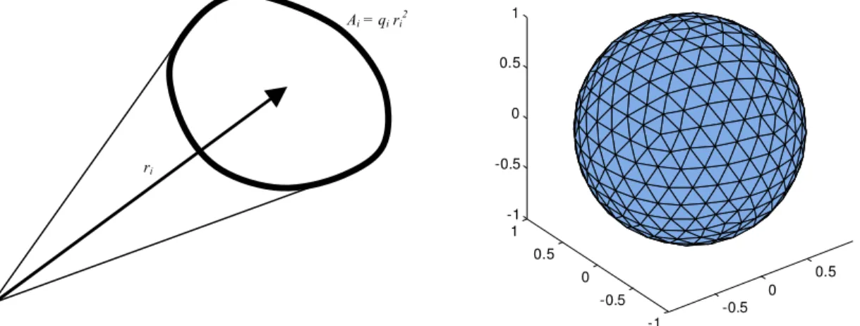
The surface of the sphere is represented by a large number of distinct points and each is associated with a surface area as shown in Figure 3. The size of the incremental surface area is ai = qi ri2, where qi is a constant that depends on the choice for the layout of the
surface points. The elemental volume is approximately vi = (1/3) qi ri3 and its centre of
mass is located a distance approximately r¯i = (3/4) ri from the origin.
The spherical iceberg geometry was represented as a series of pentagons and hexagons in a form known as the Bucky ball. In the present characterization, each pentagon is
subdivided into five triangles and each hexagon is divided into six triangles. Each of the triangles was subdivided further into four triangles, as shown in Figure 4. All of the angular geometry was developed using a unit radius sphere and scaled to account for the mean radius. The incremental surface area was determined by bisecting each edge to form a polygon (pentagon or hexagon), from which the parameter, qi, was calculated.
Centre of Mass
The centre of mass can be defined in terms of the incremental volumes and their positions (Eq.10) x¯ = [∑r¯ i cosθi cosφj vi] /∑ vi ; y¯ = [∑r¯ i sinθi cosφj vi] /∑ vi ; z¯ = [∑r¯ i sinφj vi] /∑ vi
Figure 3 Characterization of area associated with surface point
-0.5 0 0.5 -1 -0.5 0 0.5 1 -1 -0.5 0 0.5 1
Figure 4 Surface points on unit sphere are vertices of triangles
To preserve the centre of mass at the origin, it is necessary for x¯ = y¯ = z¯ = 0. Ideally, the conditions on the centre of mass should be solved simultaneously with Eq. 1 – 8 to yield the radii r. Practically, this is difficult since centre of mass relationships involve fourth powers of ri and a Lagrange multiplier approach does not yield a simple solution for r.
In practice, a numerical approach was used to generate a random vector e, then it was shuffled until a trial was found to satisfy a specified tolerance on the location of the centre of mass. Tests indicate there is no spatial correlation introduced in the shuffled vector e that minimizes x¯ , y¯ and z¯ , thereby preserving the randomness of the elements of
e. In practice, the calculated variance, σs2, was found to approximate, σe2, and was not
biased for the shapes that best preserved the centre of mass. Iceberg Orientation
Once an iceberg shape is generated, its orientation and waterline elevation are estimated using an approximate technique. An initial guess was made for the waterline elevation, total iceberg weight and buoyancy were calculated, an iterative procedure was used to calculate the waterline to balance weight and buoyancy, and hydrostatically correct centres of mass and buoyancy were calculated. This was done for many potential iceberg orientations and waterplane moments of inertia were calculated for each at sixteen
directions. A stable orientation was determined from those with the largest metacentric heights (i.e. most stable) and where the centres of mass and buoyancy were
approximately in line. This approach is approximate and will be revised in future.
PARAMETER ESTIMATION
Characterization of DIGS Icebergs
The below water contours were spaced 5 m for iceberg “Gladys” and 10 m apart for iceberg “Julianna”, while the above water contours had a vertical resolution of up to 2 m. Iceberg “Gladys” had a waterline length of 165 m, a waterline width of 150 m, a height of 30 m and a draft of 110 m, while iceberg “Julianna” had a waterline length of 292 m, a
ri
waterline width of 258 m, a height of 70 m and a draft of 170 m. The centre of mass was estimated by assuming the icebergs consisted of stacked right cylinders, each having the plan shape of the contour. The height of each cylinder was determined by extending it vertically, half the distance to the adjacent contours above and below it. The area and centre of mass of each cylinder was used to obtain the overall centre of mass.
The unit sphere was then placed at the centre of mass of the iceberg and the radii were extended to meet the iceberg contours. The interpolated surface points for the radial representation are shown in Figure 5 for iceberg “Julianna”. Recognizing the potential deficiencies in the surface area coverage, mean radii of 72.1 m and 135.3 m were
determined for the two icebergs. The deviations from the mean surface were determined to yield the distributions for “Julianna” shown in Figure 6. The standard deviations of the radii were calculated to be 12.6 m and 35.6 m for the two icebergs. The radial surface representations can also be viewed using the surface triangles as shown in Figure 5.
Figure 5 Iceberg “Julianna”, showing measured contours and surface points associated with radial representation; triangular patch representation of surface points
Figure 6 Distributions associated with radial representation of iceberg “Julianna”
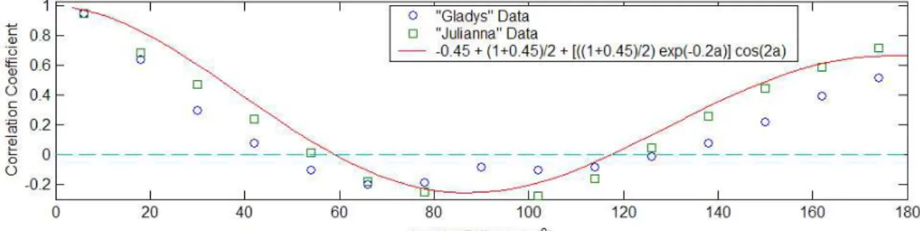
Figure 7 Spatial correlations as a function of angular separation and approximate fit for DIGS icebergs
Calculation of Model Parameters
The spatial covariance matrix, C, with elements, cij, defines the relationship between the
deviations si and sj. As shown in Figure 2, points i and j are separated by an angle αij. If
the deviations have the same properties all around the iceberg, then the covariance can be expressed in terms of the separation angle αij. Since the angle between any two points on
the sphere never exceeds π radians (180°), the covariance or correlation function is symmetric about π. The form of the correlation function was determined by binning the cross-correlation of measured radius deviations (si = ri – r0), according to angular
separation around the surface of the sphere. The results are shown in Figure 7 for the two icebergs.
In spite of differences in shape between the two icebergs, their correlation functions are similar. The function
(Eq.11) ρij = ρmin + (1–ρmin)/2 + [(1–ρmin)/2] exp(–f αij) cos (2 αij)
was used to represent the correlation, ρij, between radii at surface points i and j as a
nction of angular separation αij. Parameters f = 0.2 and ρmin = -0.45 provided a
reasonable fit. fu
The correlation matrix, ρ, was generated from Eq. 11 using the angular separations between points on the unit sphere, from which the matrix, B, was calculated. The distribution of residuals, e, was determined from the deviations, s, and the matrix, B, using Eq. 4. Figure 6 indicates that parameter, e, is well represented by a normal distribution. Coefficients of variation for e of 0.18 and 0.26 were calculated for the two icebergs analyzed and a value of 0.2 was assumed for subsequent iceberg generation. By choosing correlations as a function of angular separation, there is an implicit
assumption that shape deviations are not scale dependent. In future, it may therefore be necessary to characterize the various shape parameters for different iceberg sizes. Furthermore, the distribution of the random deviations and consequently the shape
parameters may be found to vary with the iceberg shape categorization, particularly in the case of tabular and drydock icebergs.
hape Generation
Many complete iceberg shapes were generated using the procedure and parameters
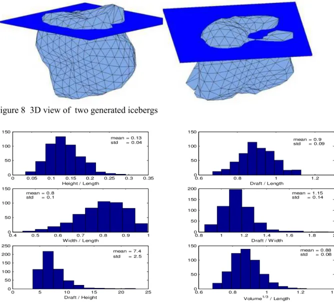
outlined above. Three dimensional views of two of these icebergs are shown in Figure 8. Since the information used to generate these icebergs was derived only from two icebergs profiled during the DIGS program, the generated shapes are biased to the specific
morphological features of these icebergs. As well, there is clearly no basis to establish a size dependence on the correlation function based on data from only two icebergs. Consequently, the icebergs have been generated in a non-dimensional sense with a unit
ndex Dimensions
length, waterline width height and draft have been
e in
ONCLUSIONS
ent of index dimensions indicates the proposed approach can apture the salient features of iceberg shape using a relatively simple statistical model APPLICATION OF THE MODEL
S
mean radius. In practice, the generated icebergs can be scaled, for example, by waterline length. No scale is shown on the plots.
I
he relationships between waterline T
calculated in numerous other studies. Dimensional relationships based on over 500 generated icebergs are illustrated in Figure 9. The average width was found to be 0.8 times the length, which is in line with the extensive measured data set. The distribution is bounded on the right since the waterline width is always less than or equal to the length. Width relationships from some measured sources may be inaccurate when other than aerial data are used. The draft was calculated to be 0.9 times the waterline length on average, which is more than the measured ratio of closer to 0.7. The height was found to be approximately 1/8 of the waterline length and 1 /7 of the draft, both of which ar
line with measurements. C
A preliminary assessm c
Figure 8 3D view of two generated icebergs 0 0.05 0.1 0.15 0.2 0.25 0.3 0.35 0 50 100 150 0.6 0.8 1 1.2 0 50 100 150
Height / Length Draft / Length
mean = 0.13 std = 0.04 mean = 0.9std = 0.09 0.4 0.5 0.6 0.7 0.8 0.9 1 0 50 100 150 0.8 1 1.2 1.4 1.6 1.8 2 Width / Length mean = 0.8 std = 0.1 0 50 100 150 200 Draft / W idth mean = 1.15 std = 0.14 0 5 10 15 20 25 0 50 100 150 200 250 Draft / Height mean = 7.4 std = 2.5 0.6 0.8 1 1.2 1.4 0 50 100 150 Volume1/3 / Length 0.88 0.08
elationships between iceberg key iceberg dimensions
tabular and drydock shapes. Without doubt, there are likely to e differences in iceberg shape with increasing size, particularly for very large tabular
l development, the statistical model assumed that the mean iceberg shape could be represented using a sphere. Clearly, this will not be appropriate for certain
mean = std =
Figure 9 Simulated r
RECOMMENDATIONS
The present study dealt with data from only two icebergs. To fully represent iceberg geometry, data from many icebergs are required. Data acquired as part of offshore initiatives for the Hibernia development in the early 1980s, at Terra Nova in 2002 and 2003 will greatly improve the statistical representation of iceberg shape.
In future work, a key aspect will be to consider the potential differences between the attributes of icebergs with
b
icebergs. In this initia
classes of icebergs and a better form may be required. A single correlation function w used to represent changes in shape around the iceberg. To properly account for local surface features, it ma
as y be appropriate to refine this characterization.
An approximate method was used to find stable iceberg positions. This part of the approach needs to be refined and a method using detailed iceberg surface information is recommended.
ACKNOWLEDGEMENTS
This project was funded by the Panel on Energy Research and Development (PERD) Ice-Structure Interaction Activity. Anne Barker (CHC/NRCC project manager) and Garry Timco (CHC/NRCC manager of PERD programs) encouraged the initiative. A number of years ago, Ian Jordaan (Memorial University of Newfoundland) suggested the
statistical characterization of iceberg shape and some of the initial ideas were developed with his encouragement.
REFERENCES
Croasdale, K., Brown, R., Campbell, P., Crocker, G., Jordaan, I., King, A., McKenna, R. and Myers, R. (2001) Iceberg risk to seabed installations on the Grand Banks, in Proc. POAC'01, Vol. 2, pp 1019-1028, Ottawa, Canada, 2001.
Dobrocky Seatech (1984) Iceberg field survey 1984, Mobil Hibernia Development Studies.
Fuglem, M., Muggeridge, K., and Jordaan, I.J. (1998) Design load calculations for iceberg impacts, in Proc. ISOPE Conference, Montreal, Vol. 2, pp. 460-467. Hodgson, G.J., Lever, J.H., Woodworth-Lynas, C.M., Lewis, C.F. (1988) The dynamics
of iceberg grounding and scouring (DIGS) experiment and repetitive mapping of the eastern Canadian continental shelf, ESRF Report No.094.
PERD (1999) Compilation of iceberg shape and geometry data for the Grand Banks region, PERD/CHC Report 20-43 by CANATEC Consultants Ltd., ICL Isometrics Ltd., CORETEC Inc. and Westmar Consultants Ltd.
PERD (2000) Study of iceberg scour & risk in the Grand Banks region, PERD/CHC Report 31-26 by K.R Croasdale & Associates Ltd., Ballicater Consulting Ltd., Canadian Seabed Research Ltd., C-CORE, and Ian Jordaan & Associates Inc. PERD (2004a) Development of iceberg shape characterization for risk to Grand Banks
installations, PERD/CHC Report 20-73 by Richard McKenna.
PERD (2004b) Determination of iceberg draft and shape, PERD/CHC Report 20-75 by Oceans Ltd.
McKenna, R.F., Crocker, G.B. and Paulin, M.J. (1999) Modelling iceberg scour
processes on the northeast Grand Banks, in Proc. 17th International Conference on Offshore Mechanics and Arctic Engineering (OMAE), St. John’s.
McKenna, R., Crocker, G., King, T., Brown, R. (2001) Efficient characterization of iceberg shape, in Proc. CANCAM, St. John’s.