Observed and simulated depletion layers with southward IMF

HAL Id: hal-00317448

https://hal.archives-ouvertes.fr/hal-00317448

Submitted on 14 Jun 2004

HAL is a multi-disciplinary open access

archive for the deposit and dissemination of

sci-entific research documents, whether they are

pub-lished or not. The documents may come from

teaching and research institutions in France or

abroad, or from public or private research centers.

L’archive ouverte pluridisciplinaire HAL, est

destinée au dépôt et à la diffusion de documents

scientifiques de niveau recherche, publiés ou non,

émanant des établissements d’enseignement et de

recherche français ou étrangers, des laboratoires

publics ou privés.

IMF

N. C. Maynard, W. J. Burke, J. D. Scudder, D. M. Ober, G. L. Siscoe, W. W.

White, K. D. Siebert, D. R. Weimer, G. M. Erickson, J. Schoendorf, et al.

To cite this version:

N. C. Maynard, W. J. Burke, J. D. Scudder, D. M. Ober, G. L. Siscoe, et al.. Observed and simulated

depletion layers with southward IMF. Annales Geophysicae, European Geosciences Union, 2004, 22

(6), pp.2151-2169. �hal-00317448�

SRef-ID: 1432-0576/ag/2004-22-2151 © European Geosciences Union 2004

Annales

Geophysicae

Observed and simulated depletion layers with southward IMF

N. C. Maynard1, W. J. Burke2, J. D. Scudder3, D. M. Ober1, G. L. Siscoe4, W. W. White1, K. D. Siebert1, D. R. Weimer1, G. M. Erickson4, J. Schoendorf1, and M. A. Heinemann2

1_{ATK Mission Research, Nashua, New Hampshire, USA}

2_{Air Force Research Laboratory, Hanscom Air Force Base, Massachusetts, USA} 3_{Department of Physics and Astronomy, University of Iowa, Iowa City, Iowa, USA} 4_{Center for Space Physics, Boston University, Boston, Massachusetts, USA}

Received: 16 June 2003 – Revised: 21 January 2004 – Accepted: 9 February 2004 – Published: 14 June 2004

Abstract. We present observations from the Polar

satel-lite that confirm the existence of two types of depletion lay-ers predicted under southward interplanetary magnetic field (IMF) conditions in magnetohydrodynamic simulations. The first depletion type occurs along the stagnation line when IMF BX and/or dipole tilt are/is present. Magnetic

merg-ing occurred away from the equator (Maynard et al., 2003) and flux pile-ups developed while the field lines drape to the high-latitude merging sites. This high-shear type of deple-tion is consistent with the depledeple-tion layer model suggested by Zwan and Wolf (1976) for low-shear northward IMF con-ditions. Expected sites for depletion layers are associated with places where IMF tubes of force first impinge upon the magnetopause. The second depletion type develops pole-ward of the cusp. Under strongly driven conditions, magnetic fields from Region 1 current closure over the lobes (Siscoe et al., 2002c) cause the high-latitude magnetopause to bulge outward, creating a shoulder above the cusp. These shoul-ders present the initial obstacle with which the IMF inter-acts. Flow is impeded, causing local flux pile-ups and low-shear depletion layers to form poleward of the cusps. Merg-ing at the high-shear dayside magnetopause is consequently delayed. In both low- and high-shear cases, we show that the depletion layer structure is part of a slow mode wave stand-ing in front of the magnetopause. As suggested by South-wood and Kivelson (1995), the depletions are rarefactions on the magnetopause side of slow-mode density compressions. While highly sheared magnetic fields are often used as prox-ies for ongoing local magnetic merging, depletion layers are prohibited at merging locations. Therefore, the existence of a depletion layer is evidence that the location of merging must be remote relative to the observation.

Key words. Magnetospheric physics (magnetopause, cusp

and boundary layers; magnetosheath; magnetospheric con-figuration and dynamics)

Correspondence to: N. C. Maynard ([email protected])

1 Introduction

The existence of depletion layers near the magnetopause was first suggested by Midgely and Davis (1963), who reasoned that the magnetic field draping around the magnetopause sur-face would be constrained to flow in one direction while plasma could flow in all directions. This leads to local mag-netic field intensifications and attendant plasma density de-creases. Zwan and Wolf (1976) explicitly calculated plasma distributions in the vicinity of the magnetopause to model de-pletions near the subsolar stagnation point. The model does not allow for magnetic merging (Dungey, 1961) and applies to cases of northward interplanetary magnetic field (IMF). Two mechanisms cause depletion layers. First, deflection by the bow shock around the magnetopause causes plasma to move along the magnetic field lines away from the nose. Second, compressional forces exerted on magnetic flux tubes squeeze plasma away from the subsolar magnetopause along draped field lines. This results in enhanced magnetic fields coupled with decreased plasma density. They predicted de-pletion factors, ratios of the post-shock to local densities, be-tween 3 and 4. Analyses of IMP-6 measurements showed de-pletion factors that varied from 1.4 to more than 2 (Crooker et al., 1979).

If merging is occurring at the subsolar magnetopause, plasma flow in the X direction does not completely stagnate, eliminating magnetic field pileup. In a sense, the existence of a depletion layer is an indicator of a locally closed mag-netopause, since magnetic merging would carry away the magnetic flux and prevent its buildup. Depletion layers are common near the nose of the magnetopause when the IMF is northward or nearly in the direction of the Earth’s dipole magnetic field (low-shear condition). Depletion layers have also been observed for high shear conditions (IMF clock an-gle greater than 60◦) (Anderson and Fusilier, 1993). Mag-netic merging is commonly believed to be the primary means of coupling the solar wind energy into the magnetosphere. It is important to understand why some high-shear magne-topause crossings have depletion layers, since their existence

seemingly precludes merging, at least locally. In this pa-per we explore the causes of high magnetic-shear depletion layers by comparing satellite observations with magnetohy-drodynamic (MHD) simulated predictions of the Integrated Space Weather model (ISM) code (White et al., 2001).

AMPTE/IRM data indicate that depletion layers are com-mon at a low-shear (≤30◦) magnetopause (Phan et al., 1994). With a high-shear (≥60◦) magnetopause they identified no systematic behavior. Anderson and Fuselier (1993) reported that depletions could be found for all orientations of the IMF but that decreases were small when the IMF had a south-ward component. Anderson et al. (1997) defined a parame-ter D=ER/ESW as an indicator of merging efficiency. Here

ER is the reconnection electric field and ESW is the solar

wind electric field. D=1 corresponds to no depletion while D=0 corresponds to maximum depletion. They showed that the merging efficiency was a factor of 3 larger during AMTE/IRM (Phan et al., 1994) than AMPTE/CCE (Ander-son and Fusilier, 1993) observations. This result was ad-vanced as a reason why Phan et al. (1994) failed to detect systematic depletions during high shear situations. They as-sociated the cause to a 3-fold higher β for the CCE events. Hence, they expect that high-shear depletion layers occur with high solar wind densities. Farrugia et al. (1995) con-cluded that depletion layers were possible for high magnetic shear whenever the upstream Alfv´en mach number was low. Maynard et al. (2003) used Polar and Cluster data to show that merging often occurs at high latitudes. They described detailed characteristics of an event on 12 March 2001, in which a depletion layer was observed just outside of the magnetopause while merging was occurring poleward of the spacecraft. The event occurred during a high-magnetic-shear interval when the IMF clock angle was ∼140◦_.

Wu (1992) was first to report depletion layers in MHD simulations. The layer was thicker but the depletion fac-tor (1.2) was less than predicted by Zwan and Wolf (1976). More recently, Siscoe et al. (2002a) used ISM simulations to demonstrate the systematic variations of depletion layers with IMF clock angles. Depletion factors >3 appear for all cases with the shear ≤90◦. The thickness of depletion layers decrease with increasing IMF clock angles. Wang et al. (2003) showed from MHD simulations for northward IMF that the depletion layer existed all around the dayside and be-came thicker away from noon. It was also well defined in the noon-midnight plane past 40◦magnetic latitude. In this pa-per we wish to emphasize the generality of Zwan-Wolf deple-tions and related effects at all locadeple-tions on the magnetopause where the local magnetopause is “passive” (not merging) and particularly at the subset of such locations where the IMF first encounters the magnetopause as a blunt body.

Siscoe et al. (2002a) also pointed out that in ideal, incom-pressible MHD the stagnation point becomes a line along which the plasma velocity is identically zero. In the absence of merging, the magnetic field that passes through a stagna-tion point lies on the magnetopause surface and is an MHD mandated stagnation line (Sonnerup, 1974). As such it is a velocity separator line along which the plasma flow diverges.

Motivated by the observation of a density enhancement in front of the magnetopause (Song et al., 1990; 1992), South-wood and Kivelson (1992) argued that a slow MHD shock must form in the magnetosheath behind the bow shock. De-pending on pressure anisotropy, it should stand in the sheath flow ahead or behind the intermediate wave (rotational dis-continuity) at the magnetopause. A standing slow mode wave would enhance the density and decrease the magnetic field, opposite to the predictions of Zwan and Wolf (1976). Southwood and Kivelson (1995) recognized that the observa-tions of Song et al. (1990, 1992) and the mechanism of Zwan and Wolf (1976) both manifest slow mode properties, namely a fluctuation in 1|B|=−α1n. They suggested that the two models could be reconciled if the slow-mode waves were de-tached from the magnetopause. Behind the dede-tached shock, magnetic fields should deflect toward the magnetopause. En-hanced magnetic fields and plasma depletions develop at the nose, earthward of the plasma compression at the wave front. The J ×B force of the current in the wave results in a net force that deflects flow away from the nose. We note fur-ther in this vain that the wave discussed by Southwood and Kivelson and the depletion predicted by Zwan and Wolf may be viewed as one half cycle of a slow mode disturbance that should be expected in front of any locally closed portion of the magnetopause.

Region 1 current streamlines close through the high lat-itude boundary layer of the magnetosphere (Siscoe et al., 1991, 2000). These streamlines come out of the dusk side ionosphere, follow magnetic field lines to near the mag-netopause in the equatorial region, curl up over the high-latitude magnetopause to the dawn side near equatorial re-gion, and then follow magnetic field lines back to the iono-sphere as morning side region 1 currents. A similar loop is located in the Southern Hemisphere. Both loops con-tribute to the weakening of the magnetic field at the sub-solar magnetopause and the increase of it in the lobe. Under strongly driven conditions, the lobes bulge out sunward and the cusps move equatorward (Raeder et al., 2001). Siscoe et al. (2002b) describe the bulge (or deformation of the mag-netopause boundary) located above the cusp as a “shoulder”, which is the terminology used here. The lobe magnetic field is nearly in the same direction as the draped IMF; hence, this is a locally low-shear boundary encountered above the cusp. In the following sections we demonstrate that the depletion layer reported in Maynard et al. (2003) occurred near a velity separator. ISM simulations show that the observations oc-curred in a region where depletion is expected. We then use ISM simulations to show that under strongly driven condi-tions with southward IMF, low-magnetic-shear shoulder con-figurations develop poleward of the cusp. These shoulders impede the flow of magnetic flux toward the nose, requiring the field lines to drape around the shoulder before they can merge at the dayside magnetopause. In so doing they cre-ate a depletion layer above the cusp. Polar measurements confirm this ISM prediction. Both types of depletion layers are possible under high-shear, sub-solar magnetopause con-ditions. The first is tied to merging away from the sub-solar

region. The second type inhibits dayside merging and is a possible mechanism for understanding the saturation of the ionospheric potential under strongly driven conditions (Sis-coe et al., 2002b, c).

2 Measurements

In 2001 Polar’s apogee (9 RE) was near the equator. As

a consequence, for long intervals in March-April the orbit skimmed from south to north, along the dayside magne-topause. Thus, variations in phenomena observed by Polar are primarily temporal rather than spatial. Information about radial scale sizes is lost. However, Polar closely monitors magnetopause responses to temporal changes of the IMF and solar-wind pressure. Several sensors on Polar are used in this study. The Hydra Duo Deca Ion Electron Spectrometer (DDIES) (Scudder et al., 1995) consists of six pairs of elec-trostatic analyzers looking in different directions to acquire high-resolution energy spectra and pitch-angle information. Full three-dimensional distributions of electrons with ener-gies between 1 eV and 10 keV and ions with enerener-gies per charge ratio of 10 eV q−1 to 10 keV q−1 were sampled ev-ery 13.8 s. The electric field instrument (EFI) (Harvey et al., 1995) uses a biased double probe technique to measure vector electric fields from potential differences between 3 or-thogonal pairs of spherical sensors. This paper presents mea-surements from the long wire antennas in the satellite’s spin plane. The Magnetic Field Experiment (MFE) (Russell et al., 1995) consists of two orthogonal tri-axial fluxgate mag-netometers mounted on non-conducting booms. The electric and magnetic fields were sampled 40 and 8 s−1_{, respectively.} Data presented in this paper were spin averaged using a least-squares fits to a sine function.

The Advanced Composition Explorer (ACE) spacecraft monitors interplanetary conditions while flying in a halo or-bit around the L1point in front of the Earth. The solar wind velocity was measured by the Solar Wind Electron, Proton, and Alpha Monitor (SWEPAM) (McComas et al., 1998). A tri-axial fluxgate magnetometer measured the interplanetary magnetic field vector (Smith et al., 1998).

3 The Integrated Space Weather Prediction Model

The Integrated Space Weather Prediction Model (ISM) op-erates within a cylindrical computational domain whose ori-gin is at the center of the Earth. Its domain extends 40 RE

sunward, and 300 RE in the anti-sunward direction, and

60 RE radially from the Earth-Sun line. In simulations

de-scribed here, the cylindrical domain has an interior spherical boundary approximately located at the bottom of the E-layer (100 km). The cylindrical to spherical interface is at 3 RE.

ISM uses standard MHD equations augmented by hy-drodynamic equations in the collisionally-coupled thermo-sphere. Conceptually, as one moves toward the Earth, equa-tions transition continuously from pure MHD in the solar wind and magnetosphere to those proper to the low-altitude

ionosphere/thermosphere. The simulations discussed here contain specifically selected parameters and simplifying ap-proximations. Finite-difference grid resolution varies from a few hundred kilometers in the ionosphere to several RE near

the computational domain’s outer boundary. At the magne-topause, resolution ranges from 0.2 to 0.8 RE. Explicit

vis-cosity in the plasma momentum equation was set to zero. To approximate nonlinear magnetic reconnection the explicit resistivity coefficient ν in Ohm’s Law equation is zero if cur-rent density normal to B is less than 3.16·10−3Am−2. In re-gions with perpendicular current densities above this thresh-old, ν=2·1010m2s−1. In practice, this choice of ν leads to non-zero explicit resistivity near the subsolar magnetopause, and in the nightside plasma sheet. Dissipation, where needed to maintain numerical stability, is based on the partial donor-cell method (PDM) as formulated by Hain (1987).

In the following discussion we present the results of five simulations. The input solar wind parameters for each run are given in Table 1. Because of their negligible impact on the results and in order to reduce run times of simulations, routines in the ISM code containing thermospheric hydrody-namics and explicit chemistry between ionospheric and ther-mospheric species were not activated. Ionospheric Pedersen conductance is 6 S at the pole and varied in latitude as B−2. It is uniform in longitude. No Hall conductance was used.

4 Depletion layers with northward IMF

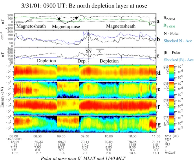
To set the stage for the depletion layers when the IMF has southward components, we first examine conditions on 31 March 2001, during a period when the IMF was strongly northward and Polar’s orbit was skimming along the dayside magnetopause near the equator. Data from 08:00 to 11:00 UT are plotted in Fig 1. Figures 1d–g present energy-versus-time spectrograms of ion energy fluxes measured by HYDRA at all pitch angles and parallel, perpendicular, and antiparallel to the local magnetic field. The plotted numbers are the av-erage of d2f/dE/dover solid angles in which data were taken. Some investigators integrate over solid angle and re-portR (d2f/dEd)das the “omnidirectional” energy flux. The entire velocity distribution at all solid angles must be sampled to make such a determination. We avoid interpo-lating and report the average of the integrand over all direc-tions sampled, which at a 13.8 s cadence covers 12 ∗ 6=72 directions distributed over a unit sphere. Figure 1a, the black trace, shows BZ measured by Polar. The green trace

indi-cates BY. In Fig. 1b the blue line indicates the solar wind

density measured by ACE and lagged by 38 min. While the lag time may vary minute-by-minute (Weimer et al., 2002), we have chosen 38 min as providing the best average match over the plotted interval. In this case the lag time is close to the advection time and is adjusted by matching clock an-gles of magnetic fields measured by Polar and ACE (Song et al., 1992). Matching clock angles provides reasonable lags for both B and density, except when IMF BX is the

Table 1. Simulation input parameters.

# Solar Wind velocity Solar wind density IMF magnitude IMF clock IMF BX Dipole

velocity (km/s) density (protons/cm3) (nT) angle (degrees) tilt (degrees)

1 350 5 5 135 negative 0

2 350 5 5 180 0 17

3 350 5 20 180 0 17

4 350 5 20 180 0 35

5 350 5 50 180 0 0

3/31/01: 0900 UT: Bz north depletion layer at nose

Magnetopause

Depletion

Polar at nose near 0° MLAT and 1140 MLT

Magnetosheath

Magnetosheath

Figure 1

f

a

b

c

d

e

g

Depletion

Dep.

Fig. 1. Example from Polar of depletions layers with IMF BZ northward. Polar was located at 0◦MLAT and 11:40 MLT. (a) The black

trace is the measured BZat Polar. The green trace is the measured BY. The larger value of BZjust outside the magnetopause is a signature

of a depletion layer. (b) The measured ion density at Polar (black) compared to the properly lagged (38 min) ion density measured at ACE upstream in the solar wind (blue). Plasma densities attributed to ACE have been multiplied by a time-varying factor appropriate for density jumps predicted by the Rankine-Hugoniot relations for the subsolar bow shock and by an additional compression factor when Polar was close to the magnetopause as predicted by Spreiter and Stahara (1985). (c) The magnetic field magnitude measured at Polar (black) and at ACE (blue). ACE magnetic field measurements were multiplied by the time-varying Rankine-Hugoniot factor appropriate for the magnetic field jumps at the subsolar bow shock. (d–g) Ion energy spectrograms showing the total, parallel (pitch angles 0–30◦), perpendicular (75– 105◦) and antiparallel (150–180◦) ion fluxes ((cm2−s−sr−1E/E)−1). Three intervals noted by X, Y, and Z indicate the data on which the regression analyses of Fig. 11 were performed.

3/12/01: Separator depletion layer – +By

Magnetopause

Depletion

Polar postnoon at 18° MLAT and 1312 MLT

IMF clock angle

near 140°

Figure 2

f

a

b

c

d

e

g

Fig. 2. Example of a depletion layer for negative BZ and positive BY in the same format as Fig. 1. Polar was located at 18◦MLAT and

13:12 MLT.

magnetic fields measured by Polar and ACE with the same time delay. To make the comparisons with Polar data, it is necessary to adjust the ACE density and magnetic field for effects of the bow shock. The ACE magnetic field and so-lar wind density have been multiplied by time varying fac-tors calculated using the reduction of the Rankine-Hugoniot equations by Whang (1987), which predicts the jump factors based solely on the upstream conditions. As such, the values represent the expected magnetosheath density and magnetic field just inside the bow shock. All factors were calculated for the conditions at the nose. Typical factors for density range between 3 and 4. The magnetic field factor is more variable, depending on whether the shock is more perpendic-ular or parallel. They range from 1 for a purely parallel to the factor appropriate for the density with a perpendicular shock. ACE density measurements were adjusted to allow for lati-tudinal variations of the compressed magnetosheath plasma, as prescribed by Spreiter and Stahara (1985). No further ad-justment was made on the ACE magnetic field since their compression depends on several factors, negating possible

improvements with a simple change. Hydra densities were calibrated against those measured by ACE during the inter-val between 12:30 and 13:00 UT when Polar was in the solar wind.

At the location of Polar the imposed IMF turned north-ward near 08:20 UT and the magnetosheath ion distributions became increasingly dominated by the perpendicular fluxes, or “pancake” shaped, as antiparallel and parallel fluxes disap-peared. The magnetic field’s magnitude increased by a factor of 1.7 above the shocked IMF (Fig. 1c). The density de-creased (Fig. 1b) relative to the adjusted solar wind density. The lower density and increased magnetic field just outside the magnetopause are the predicted signatures of depletion layers (Zwan and Wolf, 1976). The pancake ion distributions are a natural result of the Zwan and Wolf mechanisms. This trend continued until 08:54 UT when the spacecraft crossed the magnetopause into the boundary layer, marked by an abrupt change in ion spectral characteristics and a decrease in B and BZ. During magnetopause crossings with no

a

b

c

d

S. H.

N. H.

Dusk

Particle source compared to dawn-dusk velocity ~140° clock angle

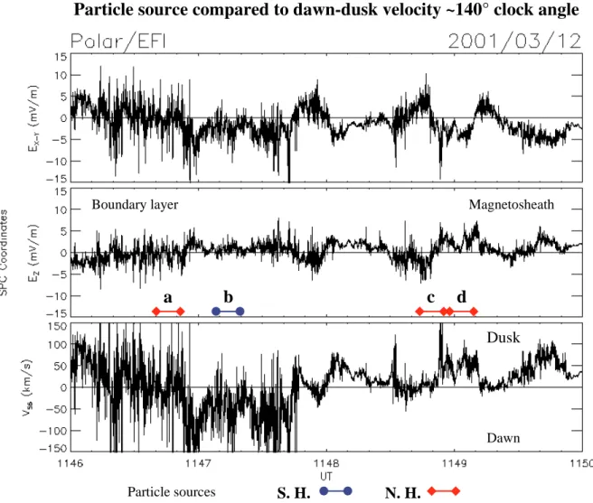
Fig. 3. High resolution (40 Hz) measurements of the 2 components of the electric field in the spin plane and the resulting drift velocity along

the spin axis, which is roughly in the Y direction (toward dusk). The letters refer to panels in Fig. 8 of Maynard et al. (2003). The circular dumbells represent intervals when fluxes are coming from below the satellite, while the diamond dumbells represent times when ions are coming from a Northern Hemisphere source above the spacecraft.

lower density boundary layer. Polar crossed back into the de-pletion layer at 09:22 UT as the increased density observed by ACE (blue trace in Fig. 1b) rapidly pushed the magne-topause inward. The depletion layer was quickly crossed, and at 09:35 UT there was a significant increase in density and a decrease in magnetic field. We return to this point in Sect. 7. After 09:40 UT the plasma density at ACE decreased and the magnetopause expanded to closer to the location of Polar, placing the satellite back into the more depressed den-sity of the depletion layer, where it remained for a consider-able interval. Compared with shocked ACE measurements, the maximum increase in B at Polar was by a factor of 2. Note that at both ends of Fig. 1c the magnetic field magnitude returns to close to the shocked IMF value, while in Fig. 1a the Z component is southward, favorable to dayside merging with no depletion. Hence, variations in measurements at Po-lar reflect temporal responses to boundary motions and the solar wind drivers. However, we cannot use Polar measure-ments to determine the thickness of the depletion layer.

The examples with southward IMF components that fol-low show data in the same format as Fig. 1. Evidence for de-pletion layers include (1) ion distributions favoring perpen-dicular pitch angles, (2) densities at Polar below the shocked ACE values, and (3) increased magnetic fields above the shocked ACE values. Ion distributions in the sub-solar mag-netosheath become more pancake shaped as the magnetic flux piles up in the stagnated region.

5 Velocity separator depletion layers

Maynard et al. (2003) identified a merging event at high lat-itudes during the Polar magnetopause crossing at 11:48 UT on 12 March 2001. Accelerated ions and Poynting flux car-ried by Alfv´en waves were observed coming from poleward of the spacecraft, on both the magnetosphere and tosheath sides of the current layer. After crossing the magne-topause Polar entered a region of low plasma density within the magnetosheath. Figure 2 presents HYDRA and MFE

data from Polar for this crossing (some of which is repeated from Fig. 6 of Maynard et al., 2003). Figure 2 is presented in the same format as Fig. 1. Figures 2d–g show ion energy fluxes in spectrogram formats. Figure 2a presents IMF BY

and BZcomponents measured by Polar as being comparable

with an average clock angle of ∼140◦. A positive IMF BX

also was present. Note that just outside the magnetopause crossing the parallel and anti-parallel ion fluxes were very small. Perpendicular fluxes dominated but at reduced levels compared to those detected after 12:15 UT. Figure 2b com-pares the density measured by Polar with that measured by the ACE satellite. Here ACE data were lagged by 63 min, which proved optimal for the magnetopause crossing as de-termined in Maynard et al. (2003). Ion densities detected just outside the magnetopause were less than or comparable to those of the shocked solar wind as observed by ACE. B remained above the shocked IMF value until a major IMF decrease occurred near 12:18 UT. The maximum enhance-ment of the magnetic field was by a factor of 1.9. Reduced densities and corresponding enhancements in B are clear in-dications of depletion layers. Note that the density minimum observed at 12:00 UT does not correspond to a change in the solar wind density, but to an increase in the total magnetic field (Fig. 2c). Temporal changes in the depletion, such as observed at 12:00 UT, most likely reflect a small movement of the magnetopause, placing the satellite deeper inside the layer.

Signatures of accelerated ions appear in three of the four particle distributions shown in Fig. 8 of Maynard et al. (2003), to demonstrate that merging was occurring at high latitudes to the north of the spacecraft. The accelerated ions in the other example came from the south. This suggests that Polar was located near the velocity separator line, or the magnetic field line that passes through the stagnation point at the nose. Sonnerup (1974) showed that in incompress-ible MHD the stagnation point stretches into a line along B. Later, Siscoe et al. (2002a) demonstrated this effect with the ISM code. On the dawn (dusk) side of this line plasma flows toward dawn (dusk). To test the conjecture that Polar was in the vicinity of the stagnation line, Fig. 3 plots the two electric field components measured in the spin plane of the spacecraft and the velocity along the spin axis calculated using those components during the magnetopause crossing. The spin axis points close to the dawn-dusk direction. The intervals over which the particle distributions shown in Fig. 8 of May-nard et al. (2003) were taken are noted with square (circular) dumbbells for distributions originating north (south) of the spacecraft. The letters refer to the labels in Fig. 8 of Maynard et al. (2003). Where the particle source was south (north) of the spacecraft or from the Southern (Northern) Hemisphere, the velocity was toward dawn (dusk), as anticipated. This is consistent with Polar being located near the stagnation line or velocity separator.

Since incoming magnetic flux in the magnetosheath drapes over the magnetopause before reaching high-latitude merg-ing sites, flux pile up must occur near this stagnation line and a depletion layer should form (Midgely and Davis, 1963;

Zwan and Wolf, 1976). Positive IMF BXcauses flux to

en-counter the stagnation line north of the equator first, enhanc-ing the flux pile up at that point. Note that if component merging had been occurring near the equatorial region, no flux pile up would have developed as field lines would have been immediately dragged in the dawn or dusk direction.

To explore this scenario, we utilized an existing ISM simu-lation (Simusimu-lation 1 in Table 1) with equal magnitudes for all IMF components; BXand BZnegative and BY positive. The

negative IMF BX places the first contact point to the

stag-nation line south of the equator on the dawn side of noon, comparable to the observations at Polar on the dusk side of noon north of the equator with IMF BX>0. Figure 4a shows

ion velocity vectors and contours of BZ in the Y Z plane at

X=9.9 RE. The tan colored region represents the nose of

the magnetosphere with positive BZ; the color blue indicates

negative BZand open field lines. In the region of open field

lines noted by arrows, Figs. 4b and c show decreased density and increased magnetic field, respectively. The simulation provides the signatures of a depletion layer in the region of the first contact with the stagnation line, comparable to the Polar measurements described above. The depletion in den-sity of about 1.3 is less than measured but comparable to val-ues of 1.3 and 1.2 reported by Wu (1992) and Lyon (1994), respectively, in depletion-layers simulations with northward IMF, using other MHD codes. The depletion is localized south of the equator and primarily in the vicinity of the stag-nation line, although it also extends across noon with some-what weaker levels of enhanced B. The negative BXin the

simulation places the first contact point south of the equator, in the prenoon sector (Fig. 4). Had the simulation run with positive IMF BX, the first contact point and strongest

sig-nature of depletion would occur north of the equator in the postnoon sector. This compares favorably with the location of Polar. The presence of IMF BXcan enhance the depletion

as does dipole tilt. Maynard et al. (2003) showed that the merging site moved off the equator and away from the point of first contact with increasing dipole tilt. IMF BX>0 at

Po-lar serves to enhance the effective dipole tilt and increase the depletion. Siscoe et al. (2002a) showed that the depletion is minimal when IMF BX=0 and the dipole axis is vertical. The

simulation has a current-dependent, explicit resistivity at the nose, which favors merging at that location. In the simulation the neutral line moved away from the subsolar region, indi-cating a strong preference for high-latitude merging when the dipole is tilted.

If IMF BY had been negative and BX positive, the

de-pletion layer would have been located on the dawn side of noon in the Northern Hemisphere. Such a case was observed briefly at ∼11:30 MLT (near 08:00 UT) on 16 April 2000, when Polar was moving northward and toward dusk along the magnetopause. Figure 5 displays similar quantities to those in Figs. 1 and 2 between 06:00 and 11:00 UT. Polar ini-tially crossed the magnetopause at 07:10 UT. Approaching the current layer on the magnetosphere side, Fig. 5a shows that the angle of B rotates to ∼45◦as the current layer is en-tered and then to 90◦IMF orientation on the outside of the

IMF: - B

; +B

; -B

Negative B

Depressed

Density

Enhanced B

magnitude

Magnetopause

nose

on open

field

lines

on closed

field lines

Magnetosphere

nose

X = 9.9 R

a

b

c

B (nT)

Magnetic field magnitude

Fig. 4. Results from a MHD sim-ulation with a constant IMF input of equal magnitude negative BX, positive

BY and negative BZ. The simulation

output is presented in the Y Z plane at X=9.9 RE, which just contacts the

nose of the magnetosphere. (a) Veloc-ity vectors are overlaid on the plane colored with BZ. Brown colors

indi-cate closed magnetosphere field lines, while blue colors indicate open magne-tosheath or boundary layer field lines.

(b) The plane is colored with the

pro-ton number density. (c) The plane is colored with the magnitude of the mag-netic field. Attention is called to the region below and to the left of center in each panel, where depressed density and enhanced B are seen on open field lines.

4/16/00: Separator depletion layer – –By

Depletion

Strongest depletion at

clock angle near 135°

Figure 5

a

b

c

d

e

f

g

Fig. 5. An example from Polar located prenoon at 30◦MLAT and 11:32 MLT in the same format as Fig. 1. The signatures of depletion are seen briefly just before 08:00 UT when IMF BY is negative and comparable to BZ. Subsequently, as the magnitude of BY decreases,

antiparallel ion fluxes and the total ion density return from merging somewhere below the spacecraft. Depletion is seen on the dusk side of noon for the opposite polarity of B_Y near 10:00 UT. Three intervals noted by X, Y, and Z indicate the data on which the regression analyses in Fig. 12 were done.

current layer. This rotation in the boundary layer is consis-tent with MHD simulations (Maynard et al., 2001). The IMF and Polar B quickly rotated from a clock angle of 90◦_{to a}

strongly negative BZ, concurrent with an increase in the

den-sity. At this prenoon local time and 22◦ _{magnetic latitude,}

the magnetosheath density followed the adjusted solar wind density, but at a slightly lower level. The magnitude of B in-creased. However, the ion fluxes were strongest in the direc-tion parallel to the magnetic field. The ion temperature was higher than that observed in the magnetosheath after the next magnetopause crossing. The solar wind density decreased near 07:30 UT, and the magnetopause briefly expanded to the location of Polar at 07:35 UT. Beyond this second outbound magnetopause crossing BY became negative and comparable

in magnitude to BZ. At this time the velocity separator

lo-cation would be prenoon in the vicinity of the satellite. Near 08:00 UT evidence of a mild depletion layer is seen in the density and magnetic field (noted by the blue bar). The

de-pletion encounter was brief, becoming most intense after a flux transfer event at ∼07:54 UT. Soon after this BY returned

to zero, and the depletion interval ended as ion densities mea-sured by Polar increased to the adjusted ACE densities.

A second region of depletion, identified by enhanced B and pancake particle distributions, appears in Fig. 5 after 09:30 UT. Polar was located near magnetic noon and at a magnetic latitude >40◦_{. B}

Y was positive, similar to the

con-ditions of 12 March 2001. Figure 4 shows that the region of depressed density and enhanced B extends to noon from the maximum near the velocity separator, suggesting that Po-lar accessed the depletion region. The depletion increased with time as evidenced by the increase in B and the de-crease in parallel and antiparallel ion fluxes until 10:10 UT. The density remained relatively constant near adjusted ACE values; however, the electron pressure and temperature (not shown) decreased commensurate with the increase in B. Near 10:20 UT an increase in the solar wind density pushed

IMF Bz = -5 nT

Effects of increased

driving with dipole tilt:

Narrows distance

between cusps

Creates a shoulder

above cusps

Cusp

Cusp

Cusp

Cusp

Shoulder

Cusp

Cusp

Shoulder

17° tilt

17° tilt

_{IMF Bz = -20 nT}

35° tilt

Figure 6

a

b

c

Magnetic field vectors Magnetic field vectors

Magnetic field vectors

100 75 50 25 0 100 50 75 25 0 B (nT) B (nT)

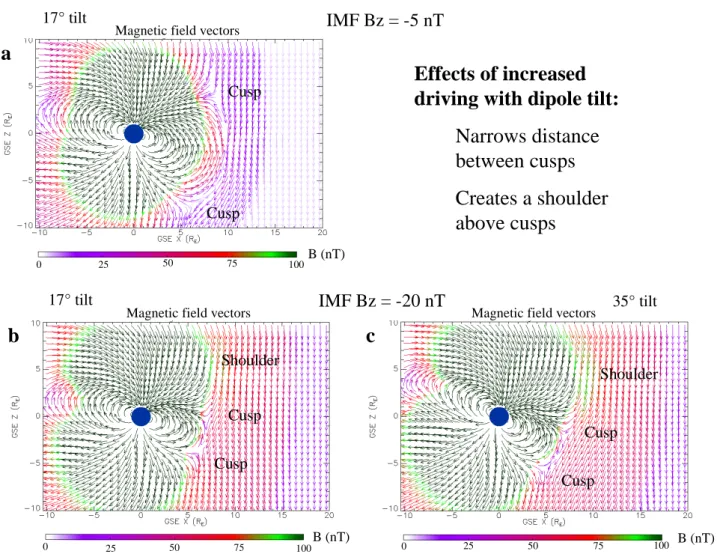
Fig. 6. Simulation of the effects of increased dipole tilt and increased magnitude of the IMF. All panels show the XZ plane at Y =0. The

arrows show the direction of the magnetic field and are colored with the magnitude. (a) and (b) have the same dipole tilt but change the IMF driver. (b) and (c) have the same input driver, but change the dipole tilt. Note that the increased IMF driver compresses the cusps together and starts to build a shoulder of enhanced magnetic field above the cusp that is tilted toward the Sun. Increasing the dipole tilt increases the size and strength of the shoulder.

the magnetopause toward the Earth, away from Polar, and a sharp increase in density was seen at Polar, located at mag-netic noon and about 45◦magnetic latitude. This sharp in-crease was similar to that observed after 09:22 UT on 31 March (Fig. 1) and the two results will be compared in Sect. 7.

Velocity-separator depletion layers are more localized than those found under northward IMF conditions, which ex-tend all around the dayside (Wang et al., 2003). They cannot form if the merging is confined to the subsolar region. Thus, their presence indicates high latitude merging. We reiterate that Polar provides no information on the thickness of a de-pletion layer. Due to the skimming nature of the trajectory, we lack knowledge about its exact relationship to the magne-topause.

6 Shoulder depletion layers

ISM simulations predict a second type of depletion layer with southward BZwhen the IMF strength increases. Maynard et

al. (2003) gives an example of merging moving away from the equator with increased dipole tilt, with a purely south-ward IMF. Recall that IMF BXadds or subtracts to the

fective dipole tilt (Crooker, 1992). Figure 6 shows the ef-fects of combining dipole tilt and increasing the IMF mag-nitude. Figure 6a shows magnetic-field vectors colored with the magnitude of the magnetic field for simulation 2 (Table 1) with 17◦dipole tilt and a −5 nT BZas the driver. The

magne-topause and cusps are evident in the vector patterns. Increas-ing the driver to −20 nT in simulation 3 (Table 1), shown in Fig. 6b, causes the cusps in the outer magnetosphere to move toward the equator, shrinking the dayside magnetosphere at sub-cusp latitudes. A shoulder, or a region of open field lines, develops above the Northern Hemisphere cusp and extends

Shoulder Depletion with Bz = -20 nT and - 35° dipole tilt

Increased B

Decreased

density

Open-IMF

boundary

Velocity

minimum

Figure 7

a

b

c

d

Magnetic field lines and velocity magnitude

Mass density Ion velocity and log B

Magnetic field lines and mass density

Fig. 7. Details of the shoulder depletion layer depicted in Fig. 6c. All panels display the XZ plane at Y =0. (a) Ion velocity vectors overlaid

on the plane colored with the log of B. (b) Traced magnetic field lines with the velocity magnitude as the background. The yellow field lines are open and connected to the Northern Hemisphere ionosphere. The green field lines are open to the solar wind on both ends. A velocity minimum is seen just inside the open/IMF boundary. (c) Mass density and (d) mass density with the traced magnetic field line overlay. The decreased density and the enhanced B seen in (a) are co-located at the open-IMF boundary.

sunward of the sub-solar magnetopause. In part, the shoul-der results from strong Northern (summer) Hemisphere re-gion 1 currents that close through the low-latitude bound-ary layer and along the high-latitude magnetopause. Fig-ure 6c shows the shoulder expanding with increased dipole tilt to 35◦. Green colored vectors extending out into the mag-netosheath above the cusp indicate the presence of a large magnetic field and the possibility of a depletion layer. The shoulder represents the first point of contact between a purely southward IMF and the magnetosphere. Magnetic field vec-tors in Figs. 6b and c are seen to drape around the shoulder.

Figure 7 displays plasma densities and magnetic fields observed near the magnetopause poleward of the Northern-Hemisphere cusp for simulation 4 (Table 1), depicted in Fig. 6c. Figure 7a plots velocity vectors over contours of the log of the magnetic field. Figure 7b traces magnetic field lines over contours of the magnitude of ion velocity. Traced field lines are colored yellow if they are open with

one foot in the Northern Hemisphere ionosphere and green if both ends connect to the solar wind. The change in color marks the open-IMF field boundary or “outer separatrix” ex-tending to an active merging separator. Because of the dipole tilt merging occurs below the equator in the Southern Hemi-sphere. Thus, the Northern Hemisphere cusp contacts the magnetosheath south of the equatorial plane. The light pur-ple in the region near X=9 and Z=1−3 REindicates an

in-crease in B in the shoulder region at the outer separatrix. The green region behind the outer separatrix in Fig. 7b rep-resents a plasma velocity minimum that occurs in a stagna-tion region where velocity vectors turn poleward and mag-netic field lines are swept back over the magnetopause. Fig-ures 7c and d show plasma density contours. Magnetic field line traces are also overlaid in Fig. 7d to highlight the outer separatrix by the change from yellow to green magnetic field lines. The reddish color overlaid by the separatrix reflects de-creased plasma density in the depletion layer. The magnetic

Increased B and magnetic pressure Decreased density Open-IMF boundary Velocity minimum

Shoulder depletion from Bz = -50 nT and no dipole tilt

Figure 8

0.5 0.8 1.1 1.4 1.7 2.0

Log B (nT) Magnetic field lines and log B

1.0 1.8 2.6 3.4 4.2 5.0

Ion mass density (kg/m3₎

Magnetic field lines and mass density

30 84 138 192 246 300

V (km/s) Magnetic field lines and velocity magnitude Magnetic field lines and magnetic pressure

0 2 4 6 8 10 E -8

Magnetic pressure (J/m3₎

a

b

c

d

Fig. 8. Shoulders develop above both cusps in simulations with no dipole tilt, but with exceptionally strong driving IMF (50 nT). The panels

display a region of the XZ plane at Y =0. Magnetic field lines displayed are open and attached to the Northern Hemisphere ionosphere. The backgrounds in (a) and (b) are the log of B and magnetic pressure, respectively. (c) The plane is colored with the mass density. (d) Velocity magnitude provides the background. The depletion layer signatures are highlighted by the arrows, and their location relative to the open-IMF boundary is provided by the traced magnetic field lines.

flux pileup and the decrease in density are clear signatures of a low-shear depletion caused by the shoulder.

If the system is driven even harder, shoulders can develop in both hemispheres with no dipole tilt and a purely south-ward IMF BZ. Figure 8 displays such a case with a

driv-ing field of −50 nT (simulation 5 of Table 1). This run is north-south symmetric and only the Northern Hemisphere is shown. Figures 8a and b show the magnetic field and mag-netic pressure overlaid with traced magmag-netic field lines. Blue colored magnetic field lines are open with one foot in the northern ionosphere. Only the first IMF (green) field line is shown, which with the last blue trace defines the outer sep-aratrix, as indicated by an arrow in each plot. Note the in-crease in magnetic field and in magnetic pressure around the separatrix. Figures 8c and d show the density and velocity magnitude overlaid with the traced magnetic field lines. De-creased plasma density and velocity are associated with in-creased magnetic field magnitude. All of these features occur

poleward of the cusp and are caused by the shoulder. From symmetry with no dipole tilt, a similar depletion layer devel-ops poleward of the Southern Hemisphere cusp.

The major magnetic storm on 31 March 2001 allowed an empirical test for the existence of shoulder-depletion layers. Figure 9 provides data for 05:00 to 08:00 UT in the same for-mat as Fig. 1. The IMF has a magnitude of 45 nT throughout this period with a clock angle near 160◦_{. At this time, the}

dipole tilted back toward the nightside in the Northern Hemi-sphere, emphasizing the shoulder in the vicinity of Polar at southern high latitudes. Note, this is a Southern Hemisphere pass in which Polar transitioned from the mantle into the high altitude cusp and then to the magnetosheath. As evidenced by the continuously negative BZ in Fig. 9a, Polar entered

the magnetosheath poleward of the cusp at 06:20 UT, with-out crossing the shrunken dayside magnetosphere (cf. Figs. 7 and 8). At Polar’s prenoon location the magnetic latitude was only −26◦, consistent with the predicted compressed dayside

3/31/01: 0630 UT: Shoulder depletion layer

Mantle Cusp Magnetosheath

Outer separatrix

Depletion

Polar prenoon at –27° MLAT and 1120 MLT – never enters dayside magnetosphere

IMF 45 nT – clock angle near 160

f

a

b

c

d

e

g

Fig. 9. Polar data from 31 March 2001, showing a shoulder depletion layer located below the Southern Hemisphere cusp in the same

format as Fig. 1. Because of the strong driving conditions Polar crossed from the mantle into the magnetosheath, not contacting the dayside magnetosphere. In this case the dipole is tilted away from the Sun.

magnetosphere and equatorward retreat of the cusps. The magnetopause contracted to inside of geosynchronous orbit (Ober et al., 2002). Intense parallel ion fluxes (Fig. 9d) at this time are products of dayside merging causing plasma to stream along the outer separatrix. Ions accelerated parallel to the magnetic field (away from the equator) and similarly di-rected parallel Poynting flux from Alfv´en waves indicate the location of an outer separatrix connected to a merging site at lower latitudes (see black bars in Fig. 9d). The magnitude of B in the magnetosheath at this location above the cusp in-creased on the magnetosheath side of the separatrix. Accel-erated O+ions were detected by the TIMAS instrument on Polar within the cusp and at the separatrix (not shown). The cutoff in O+ ion fluxes confirms Polar’s transition into the magnetosheath. Low density and lower energy perpendicular fluxes are measured between 06:20 and 06:40 UT. The den-sity is comparable to the lagged ACE denden-sity. All of these features indicate the presence of a depletion layer. As the lagged ACE density increased near 07:00 UT, the energy and

intensity of magnetosheath ions increased even more. The magnetopause boundary moved farther away from the satel-lite at that time. Later, as the solar wind density observed by ACE decreased and the magnetopause apparently expanded closer to Polar, ion fluxes measured after 07:15 UT again de-creased in energy and intensity.

Later in the day, between 15:00 and 17:00 UT, while geo-magnetic activity was still strong, Polar re-entered the mag-netosphere poleward of the Northern Hemisphere cusp. The IMF was 30 nT with a clock angle near 180◦_{. At this time the}

Earth’s dipole tilted sunward, emphasizing the formation of a Northern Hemisphere shoulder. Figure 10 presents Polar data in the same format as above. The change from posi-tive to negaposi-tive BZ near 14:30 UT occurred in the

magne-tosheath and reflects a change in the imposed IMF direction. At 16:00 UT the satellite was near magnetic noon and 47◦ magnetic latitude. The negative direction of BZis consistent

with the direction of the IMF and of open field lines above the Northern Hemisphere cusp. Accelerated antiparallel fluxes

3/31/01: 1600 UT: Shoulder depletion layer

Mantle ion dispersion Magnetosheath

IMF change

Outer separatrix – open-IMF boundary

Depletion

Polar postnoon at 47° MLAT and 1208 MLT

IMF 30 nT – clock angle near 180

Figure 10

b

a

c

d

e

f

g

Fig. 10. Polar data from 31 March 2001, inbound above the Northern Hemisphere cusp showing a shoulder depletion layer. The format is

the same as in Fig. 1. In this case (later in the day from the data shown in Fig. 9) the dipole was tilted toward the Sun, as Polar crossed from the magnetosheath to the mantle.

of ions and Poynting flux were observed, indicating a cross-ing of the outer separatrix. Subsequently, the plasma density and magnetic fields were changing, allowing for motion of the magnetopause. Two other outer separatrix crossings are identified in Fig. 10. At each separatrix crossing the mag-netic field was larger on the magnetosheath side. Through-out the period when Polar was near the IMF-open boundary, the plasma density was low and comparable to the lagged solar wind density, supporting our interpretation that Polar observed a shoulder depletion layer. Near 16:45 UT the ion fluxes became more characteristic of the mantle. The in-crease in the ACE density starting at that time recompressed the magnetosphere, returning the separatrix to the location of Polar at 16:53 UT.

These two examples provide evidence for the existence of shoulders and shoulder depletion layers. In each case the density was low in the vicinity of the IMF-open field line boundary as predicted by the simulations.

7 Depletion layer structure

Southwood and Kivelson (1995) suggested that density en-hancements and depletion layers in front of the magne-topause were complementary parts of a standing slow mode structure. Two of the depletion layer observations discussed above allowed us to test this hypothesis with both northward and southward IMF components.

To make quantitative comparisons with this slow mode concept of depletion layers and its surroundings, we have tested whether the observed density and magnetic field fluc-tuations are consistent with the proposed type disturbances. Scudder et al. (2003) developed a test for slow-mode char-acteristics of the observed time domain structures, observed using Galilean-invariant quantities. Specifically, the disper-sion relation for slow mode waves predicts that Fourier am-plitudes of the density, δρ and magnetic field variations δby

should be linearly anti-correlated:

Figure 11

X

Y

Z

Fig. 11. Linear regression fits for three intervals of 31 March 2001, labeled X, Y, and Z in Fig. 1. Normalized changes in density are plotted

as functions of normalized changes in the maximum variance component of B. Boand Norepresent values of B and N at the nominal fit

zero of the plane wave and are constrained to be within the interval. The actual zero may lie outside the interval. The function Sig(x), −1 for X<0 and +1 for X>0, is used to rectify the sign of δB so that negative values of the resulting slope represent slow-mode solutions. Sig(0)=0. The reported slope m (related to α in Eqs. (1) and (2)) is M/sin(2_bk), where M represents actual slopes obtained from the plotted lines. See Scudder et al. (2003) for more details.

Here, α>0, θBK is the propagation angle and Bois the

mag-netic field intensity for the interval. no and Po are plasma

variables occurring when the mean magnetic field is actually observed.

The usual MHD description of the slow mode as-sumes polytropic closure to determine a sound speed, Cs,

which is the proportionality constant in the relationship be-tween density and pressure fluctuations: δP =C2_sδn. Also,

C_s2=γ Po/no, where Poand noare the spatially uniform

ref-erence pressure and density. The dimensionless proportion-ality constant in Eq. (1) is determined from linear theory to be α = V 2 A (C2 s −U2) , (2)

where U is the phase velocity of the wave in the plasma rest frame. For the slow-mode branch, the denominator of Eq. (2)

is positive for all β and directions of wave propagation. To test for the slow mode signatures we compare data on the right- and left-hand sides of Eq. (1) to a linear model with-out intercept in a coordinate system determined by minimum variance analysis on B, as discussed by Scudder et al. (2003).

The ordinate of the fit is

δn(t ) ≡ n(t ) − no (3)

while the abscissa is determined by

δby(t ) =B(t ) − Byo· ˆy. (4)

A correct inference of δbyis contingent on having correctly

identified ˆy, Bo, θ. We optimize the intercept-free linear

re-gression between δn/no and sin(θBk)δby/Bo. If after

con-sideration of the errors, the regression is acceptably ranked, the best-fit slope <α>wave is compared with the theoretical

prediction of Eq. (1) evaluated at the optimal (Bo, θBk). The

regression slope, together with β, implies a correlative choice for γ (<α>). Plasma data can also be analyzed separately to determine the underlying value of for γplasmaindependent of the wave fitting described above. Our final consistency check is to show that <α>wave ≈<α>plasma. The more extensive

analysis of Scudder et al. (2003) also allows for wave pack-ets in two orthogonal directions to the principal propagation defined by the minimum variance analysis. These additional waves, which may be slow or fast mode waves, are necessary to fully reconstruct the density variation versus time profile. Since they are not necessary for this study, we have omitted them here.

Figure 11 illustrates results of the procedure performed during the three intervals of 31 March 2001, indicated by X, Y, and Z in Fig. 1. The data and optimal linear fits are given, as well as the slope-fit parameters, uncertainties, normalized

χ2, and optimized values of Bo, no and θ , and their

uncer-tainties (note that this fit procedure selects for Bo a value

that lies within the fit interval). High quality linear fits with negative slopes characteristic of slow mode waves are found by this technique, with similar values of Bo. The densities

decrease with time, as do the adjusted ACE data. The pop-ulation near the regression lines also provides information about the relative importance during each interval of plasma compression or rarefaction. If both behaviors occur in an in-terval, data points span a range in δn that straddles zero in a significant way. Conversely, in intervals principally char-acterized as compressions (rarefactions) data points cluster along the fit line primarily in the second (fourth) quadrant of the diagram. Our determinations of δn(t ) really represent our measure of δneikz(t )_{as the wave train is carried past our}

viewing position. Data points do not represent simple Fourier amplitudes of some mode, but spatially modulated functions, that cause our estimates to be distributed along a line rather than cluster about a point on the line appropriate for the ra-tio of pure Fourier amplitudes. Our diagnostic is immune to the vagaries of relative motion, fitting quantities that are Galilean invariant: the relative opposed phase of the density and magnetic field strength.

The regression analysis provides strong support for the slow mode playing a significant role in density/field varia-tions observed in all three regions. To reduce ambiguities herent in the variable densities observed by ACE, our first in-terval for analysis commenced at 09:30 UT. Negative slopes characteristic of slow-mode structures are evident on both sides of the density peak. In interval Z the slow mode slope was similar to that of interval Y, with a large percentage of the points located below the plot’s centerline. Compar-ing Fig. 11 with Fig. 1b, we conclude that when the density peak was reached (probably in the compressive phase of the wave), relative motion between the spacecraft and boundary moved Polar back into the region of stronger depletion. This interpretation is consistent with variations in Polar and ACE

B and density data shown in Fig. 1. As the magnetopause

breathed outward Polar moved back into the principal deple-tion region. That the data points fit straight lines so well is a

measure of the source’s generation of pure slow-mode waves in a nondispersive regime. There is no need for a wave packet be monochromatic as long as its constituent wave numbers lie within the same nondispersive branch. The duration that Polar remained within features suggests that a slow-mode wave is standing in front of the magnetopause, as proposed by Southwood and Kivelson (1995).

Figure 12 show data from the three intervals labeled X, Y, and Z in Fig. 5. While Fig. 11 illustrates a standard de-pletion with northward IMF, the case shown in Fig. 12 oc-curred during a relatively high shear event with southward IMF. Panel (X) confirms the presence of the slow mode wave in the interval before 08:00 UT, previously identified as a depletion. Panels (Y) and (Z) show slow-mode behavior on both sides of the large change in density imposed from the solar wind near 10:23 UT. The actual period of the rapid change was omitted. In this case the density peaks above ad-justed ACE values. The increased parallel and anti-parallel fluxes suggest that the spacecraft stayed on the outside of the slow-mode enhancement after 10:23 UT. In the subse-quent interval the fits (not shown) varied in slope and χ2 in-creased. It is conceivable that at a given time Polar could simultaneously witness compressive wave power from mul-tiple sources, thus destroying correlations recorded at succes-sive times by Polar. In the 16 April case the second depletion formed while the IMF rotated from negative to positive BY.

The density increased when a strong density enhancement, seen by the ACE, encountered the magnetopause. The in-creased dynamic pressure caused the magnetopause to move inward, allowing Polar to move from the depleted to the en-hanced density part of the standing wave. Unlike the 31 March event, there was no imposed density decrease allow-ing the magnetopause to push back toward the spacecraft. Thus, Polar observed the outer compressive portion of the slow mode wave.

Finally, we note that we found evidence (not shown) for slow-mode waves in the other illustrated depletion layers.

8 Discussion

In the previous sections we presented empirical and simu-lation evidence for the existence of two types of depletion layers forming near the magnetopause when the IMF has a southward component. In both cases Polar observations support the predictions of ISM simulation. While these de-pletion layers occur under relatively unusual circumstances, their presence in ISM simulations provides clues as to when and where they may exist. In the following we further ex-plore the implications of these findings.

8.1 Velocity-separator depletion layers

Maynard et al. (2003) provided evidence for a depletion layer developing while the IMF clock angle was about 140◦. This paper confirms that interpretation by showing a region of depleted density relative to ACE measurements near the

Figure 12

X

Y

Z

Fig. 12. Linear regression fits for three intervals of 16 April 2000, labeled X, Y, and Z in Fig. 5. See caption for Fig. 11.

location of velocity separator. ISM reveals that the deple-tion develops best in the presence of a significant BXand/or

dipole tilt. Crooker et al. (1992) showed that the effects of

BXand dipole tilt are similar and may either add or subtract,

depending on polarity. Figure 19 of Maynard et al. (2003) showed that as the dipole tilt increases, the merging site moves to higher latitudes away from the tilt. This length-ens the time for draping of the IMF field lines around the magnetopause to the high-latitude site. We suggest that pro-longed draping times allow magnetic flux to pile up and con-sequent depletion layers to form. Component merging at low latitudes is inconsistent with this flux pileup. The presence of the depletion layer supports our interpretation of observa-tions presented in Maynard et al. (2003), that magnetic merg-ing was proceedmerg-ing at high latitudes poleward of the space-craft. In any situation in which the merging site is remote and additional draping time is involved to reach that merging site, we may expect depletion to occur.

8.2 Shoulder depletion layers

We have developed evidence for the existence of shoulder de-pletion layers in the Polar data and ISM simulations. Two ef-fects occur: the dayside cusp at the magnetopause is pinched toward the equator and a shoulder develops above the cusp. Both effects can be explained as fringe-field effects from Re-gion 1 currents closing through the high-latitude ionosphere over the polar cap. Siscoe et al. (1991, 2002c) show that as-sociated current loops pass through the magnetopause above the cusp, which augment/modify the Chapman-Ferraro cur-rents in that region. These curcur-rents form a loop where the field internal to the loop has strong +X and −Z compo-nents, which adds to the magnetic field above the cusp and subtracts below the cusp. This perturbation magnetic field contributes to shoulder development. Similarly, it depresses the magnetic field in the sub-solar region. The magnetic field at the nose drops below the dipole field for IEF values of 4 mV m−1.

Sunward dipole tilts push the shoulder region forward. This increases the time required for the IMF to drape to the merging site and allows density depletions to deepen. Even at equinox the dipole tilt varies ±12◦every day, and the tilt is strongest at solstice. IMF BXcauses complementary

varia-tions (Crooker et al., 1992). The IEF phase plane is generally tilted, with large BXincreasing the tilt in the XZ plane, so

that the phase plane tilt may add or subtract from the dipole tilt to provide an effective tilt that in some cases is much greater. The IEF phase plane orientation varies on time scales of 10 s of min (Weimer et al., 2002). Thus, the depths of de-pletions may be dynamic quantities, depending on the values of all three IMF components and the dipole tilt.

8.3 Slow mode structure of depletion layers

We have examined Polar measurements for evidence of slow mode waves standing in front of the depletion layer as postu-lated by Southwood and Kivelson (1995). In fact, evidence for a density enhancement and low B appears near 12:30 UT in Fig. 2. However, it was shown in Maynard et al. (2003) that this slow-mode-like feature reflected similar variations in the solar wind and was not unique to the formation of a de-pletion layer. Figure 2c shows that magnetic fields observed at Polar track shocked values of ACE measurements quite well, confirming that the structure was imposed by the so-lar wind. Because of the skimming nature of its orbit, Poso-lar did not fully penetrate to magnetosheath features standing in front of the magnetopause, unless there were variations in the drivers. Variations in dynamic pressure change the posi-tion of the magnetopause and the relative posiposi-tion of Polar within the layer itself. In two of the cases described above, the variations were sufficient for Polar to see both the den-sity minimum and at least some of the denden-sity enhancement portions of standing slow-mode waves. The long duration spent by Polar within depletion layers is the basis for our contention that the structure is a wave standing in front of the magnetopause.

Just as the nose of the magnetopause presents an obsta-cle around which the IMF must drape, causing the depletion layer to form, so do the Region 1 current loops and their shoulders poleward of the cusp. Because shoulders inhibit inward flow until draping allows merging to occur, a deple-tion layer characterized by increased B and decrease density must form. The Southwood and Kivelson (1995) scenario would require a slow mode shock to form and stand off the magnetopause, which would turn the field. Next to the mag-netopause a rotation in B is required and the depletion layer is formed. This layer, which occurs above the cusp, is a low-shear depletion.

9 Summary

We have provide observational and MHD simulation evi-dence for the existence of depletion layers in specific regions and situations when the IMF has southward components.

We have furnished observational evidence in support of the Southwood and Kivelson (1995) hypothesis that density de-pletions (Zwan and Wolf, 1976) and enhancements (Song et al., 1990; 1992) are parts of a slow mode wave standing in front of the magnetopause. The existence of depletion layers in front of a dayside, high-shear magnetopause with south-ward IMF components requires that any merging must be re-mote from the observation. Their presence in the sub-solar region favors high latitude merging and rules out sub-solar component merging, if merging occurs on that field line. Acknowledgements. We thank F. S. Mozer, C. T. Russell, and W. K. Peterson for Polar electric field, magnetic field, and ion com-position data, and C. W. Smith and D. J. McComas for ACE mag-netic field and plasma data. We especially thank M. Kivelson for helpful discussions. This work was supported in part by AFOSR Task 2311SDA3, NASA grants NAG5-8135 (Sun-Earth Connec-tions Theory Program grant) and NASW-99014, and by the NASA Polar mission through subcontracts with the University of Califor-nia at Berkeley. The work at Iowa is supported by NASW5-7883 by the Polar Project office at NASA. The ISM was developed under sponsorship of the Defense Threat Reduction Agency, 45045 Avia-tion Drive, Dulles, VA 20166-7517.

Topical Editor T. Pulkkinen thanks a referee for his help in eval-uating this paper.

References

Anderson, B. J. and Fusilier, S. A.: Magnetic pulsations from 0.1 to 4.0 Hz and associated plasma properties in the Earth’s subsolar magnetosheath and plasma depletion layer, J. Geophys. Res., 98, 1461, 1993.

Anderson, B. J., Phan, T.-D., and Fuselier, S. A.: Relationships be-tween plasma depletion and subsolar reconnection, J. Geophys. Res., 102, 9531–9542, 1997.

Crooker, N. U.: Dayside merging and cusp geometry, J. Geophys. Res., 84, 951–959, 1979.

Crooker, N. U.: Reverse convection, J. Geophys. Res., 97, 19 363– 19 372, 1992.

Crooker, N. U., Eastman, T. E., and Stiles, G. S.: Observations of plasma depletion in the magnetosheath at the dayside magne-topause, J. Geophys. Res., 84, 869–874, 1979.

Dungey, J. W.: Interplanetary magnetic field and the auroral zones, Phys. Rev. Lett., 6, 47, 1961.

Farrugia, C. J., Erkaev, N. V., Biernat, H. K., and Burlaga, L. F.: Anomalous magnetosheath properties during Earth passage of an interplanetary magnetic cloud, J. Geophys. Res., 100, 19 245, 1995.

Hain, K.: The partial donor cell method, J. Comp. Physics, 73, 131, 1987.

Harvey, P., Mozer, F. S., Pankow, D., Wygant, J., Maynard, N. C., Singer, H., Sullivan, W., Anderson, P. B., Pfaff, R., Aggson, T., Pedersen, A., F¨althammar, C.-G., and Tanskannen, P.: The elec-tric field instrument on the Polar satellite, Space Sci. Rev., 71, 583–596, 1995.

Lyon, J. G.: MHD simulations of the magnetosheath, Adv. Space Res., 14, (7), 21–28, 1994.

Maynard, N. C., Ober, D. M., Burke, W. J., Scudder, J. D., Lester, M., Dunlop, M., Wild, J. A., Grocott, A., Farrugia, C. J., Lund, E. J., Russell, C. T., Weimer, D. R., Siebert, K. D., Balogh, A.,