HAL Id: hal-03025198
https://hal.archives-ouvertes.fr/hal-03025198
Submitted on 7 Dec 2020
HAL is a multi-disciplinary open access
archive for the deposit and dissemination of sci-entific research documents, whether they are pub-lished or not. The documents may come from teaching and research institutions in France or abroad, or from public or private research centers.
L’archive ouverte pluridisciplinaire HAL, est destinée au dépôt et à la diffusion de documents scientifiques de niveau recherche, publiés ou non, émanant des établissements d’enseignement et de recherche français ou étrangers, des laboratoires publics ou privés.
An inversion approach for analysing the physical
properties of a seismic low-velocity layer in the upper
mantle
Jie Xiao, Saswata Hier-Majumder, Benoit Tauzin, Dave Waltham
To cite this version:
Jie Xiao, Saswata Hier-Majumder, Benoit Tauzin, Dave Waltham. An inversion approach for analysing the physical properties of a seismic low-velocity layer in the upper mantle. Physics of the Earth and Planetary Interiors, Elsevier, 2020, 304, pp.106502. �10.1016/j.pepi.2020.106502�. �hal-03025198�
An inversion approach for analysing the physical properties of a
1
seismic low-‐velocity layer in the upper mantle
2 3
Jie Xiaoa, b, c,*, Saswata Hier-‐Majumderb, Benoit Tauzind, e, Dave Walthamb
4
(a) State Key Laboratory of Organic Geochemistry, Guangzhou Institute of 5
Geochemistry, Chinese Academy of Sciences, Guangzhou, 510640, China 6
(b) Department of Earth Sciences, Royal Holloway, University of London, Egham, 7
TW20 0EX, United Kingdom 8
(c) University of Chinese Academy of Sciences, Beijing 100049, China 9
(d) Université de Lyon, UCBL, ENS Lyon, CNRS, Laboratoire de Géologie de Lyon, Terre, 10
Planètes, Environnement, Villeurbanne, France 11
(e) Research School of Earth Sciences, Australian National University, Canberra, 12
Australian Capital Territory 0200, Australia 13
* Corresponding author (Jie.Xiao.2016@live.rhul.ac.uk) 14
15
Abstract 16
In this article, we propose a new inversion scheme to calculate the melt volume 17
fractions from observed seismic anomalies in a low-‐velocity layer (LVL) located atop 18
the mantle transition zone. Our method identifies the trade-‐offs in the seismic 19
signature caused by temperature, solid composition, melt volume fraction, and 20
dihedral angle at the solid-‐melt interface. Using the information derived from the 21
amplitude of P-‐to-‐S conversions beneath the western US, we show that the multiple 22
permissible solutions for melt volume fractions are correlated to each other. An 23
existing solution can be directly transformed into a different solution whilst leaving the 24
model output unaltered. Hence, the additional solutions can be rapidly derived given 25
an initial solution. The calculation of multiple solutions reveals the universal properties 26
to the whole range of solutions. A regional-‐averaged melt volume fraction of at least 27
0.5% exists in every solution. In addition, the mantle potential temperature in the 28
western US is broadly lower than 1550 K and the LVL in this region tends to be basaltic-‐ 29
rich. Using these insights, it is possible to give firm statements on the LVL and the solid 30
mantle even though a unique interpretation does not exist. 31
32
Keywords: Shear wave, low-‐velocity layer, partial melting, inverse problem, non-‐ 33 uniqueness 34 35 1 Introduction 36
The mantle transition zone (MTZ), marked by a drastic change in the physical 37
properties of the silicate mineral phases, plays a crucial role in the convective flow 38
within the mantle. Owing to the sharp changes in density and volatile storage capacity 39
across the boundaries of the MTZ, it can act as an impediment to mass transfer and 40
sights of partial melting (Bercovici and Karato, 2003; Morra et al., 2010). Indirect 41
evidence of mass transfer between subducting slabs and surrounding mantle are 42
obtained from the so-‐called ‘superdeep diamonds’ which bear geochemical signature 43
of oxygen and carbon isotopic ratios that can be generated by mixing between mantle 44
and subducting slabs at these depths. Seismic observations also support the evidence 45
of partial melting atop the MTZ. A low-‐velocity layer (LVL) located at ~350 km depth 46
has been identified just above the mantle transition zone in numerous regions around 47
the world, with lateral thickness from tens to over a few hundred kilometres (e.g. Song
48
et al., 2004; Gao et al., 2006; Courtier and Revenaugh, 2007; Schaeffer and Bostock,
49
2010; Huckfeldt et al., 2013). Characterized by 2 – 3% reductions in shear wave 50
velocities, the LVL is characterized by a sharp interface with the overlying mantle, 51
indicating the likely presence of a chemical anomaly, in particular partial melting. 52
However, quantifying the fraction of melt has remained challenging as the 53
environmental and chemical parameters, such as the mantle temperature, bulk solid 54
composition and melt geometry, are not clearly understood. 55
The 350-‐km LVL has been frequently interpreted as a seismic signature of a small 56
fraction of melt triggered by volatile elements released from subduction zones 57
(Revenaugh and Sipkin, 1994) or mantle plumes (Vinnik and Farra, 2007). Since melts, 58
characterized by zero shear modulus, disproportionately reduce shear wave velocities, 59
seismic anomalies with low velocities are often qualitatively attributed to melting. 60
Interpreting the origin of the seismic velocity anomalies in the LVL is complicated due 61
to the competing influence of several parameters. While an increase in the 62
temperature typically leads to seismic velocity reductions, the influence of bulk mantle 63
composition on seismic velocities varies with depth (Xu et al., 2008). The multiple 64
factors also likely affect each other. For instance, melting may leave a strong impact on 65
the bulk solid composition, in particular the amount of basalt. The residual anomaly, 66
defined as the difference between the observed shear velocity and the reference 67
velocity, can be attributed to the presence of melting, and used as a basis for 68
calculating the volume fraction of melt in the LVL. Hence, calculation of the melt 69
fraction requires accurate estimation of the reference seismic velocities, i.e. velocities 70
in the absence of melting for given temperature and solid composition. 71
In addition, the non-‐uniqueness in the LVL interpretations arises from the fact 72
that, in a partially molten layer, the seismic velocity reductions depend on both the 73
melting extent and the microstructure of the melt-‐bearing aggregates (Mavko, 1980; 74
von Bargen and Waff, 1986; Takei, 1998, 2002). The dihedral angle (also known as 75
wetting angle) at the solid-‐melt interface, controls the geometry of the load-‐bearing 76
framework of partially molten rocks (Hier-‐Majumder and Abbott, 2010), trading off 77
with inferred melt volume fraction . The chemical composition is also found to play a 78
moderate role in reducing the seismic speeds (Wimert and Hier-‐Majumder, 2012; Hier-‐
79
Majumder et al., 2014), and may alter the dihedral angle (Yoshino et al., 2005). The 80
numerical experiment of (Hier-‐Majumder et al., 2014) indicated the difficulties in 81
distinguishing different types of melt from the seismic observations as the fraction of 82
melt is very small. These therefore lead to extra non-‐uniqueness in the interpretation 83
of seismic anomalies. 84
A number of previous studies mitigated the issue of competing influences by 85
carrying out computationally expensive brute-‐force search to create lookup tables for 86
inferred melt volume fractions corresponding to different controlling factors (e.g. Hier-‐
87
Majumder and Courtier, 2011; Hier-‐Majumder et al., 2014; Hier-‐Majumder and Tauzin,
2017). While a brute-‐force search can produce a particular scenario of inversion, 89
application of the approach is unable to ascertain if alternative solutions exist in the 90
parameter space. Although, in principle, the entire range of solutions could be 91
discovered through repetitive use of the algorithm given different combinations of the 92
parameters, it fails to rigorously tackle the nature of variations in the inferred melt 93
volume fractions caused by changes in the other factors. Therefore, a new inversion 94
scheme is required to interpret these geophysical observations and to address the 95
theoretical drawback of previous studies. 96
Here we present a mathematical formulation that uses the implicit symmetry of a 97
petrologic model to understand the non-‐uniqueness in the melt fraction inference. The 98
results from our work provide a more reliable evaluation of the long-‐standing problem 99
in rock physics. The principle of symmetry has been successfully applied in a sequence 100
stratigraphic problem (Xiao and Waltham, 2019), showing that the whole set of 101
solutions are closely linked even when an inverse problem is non-‐linear. An existing 102
solution can be directly transformed into another solution that leaves modelling 103
products unchanged, in the same way that rotating a square by 90° can produce an 104
identical geometry. In this way, the search for all possible solutions can begin with an 105
initial solution generated through standard inversion techniques. The application of 106
the symmetry method can then allow the additional solutions to be calculated from 107
the initial solution. 108
Embedded with a predictive forward model of shear-‐velocities, our inversion 109
scheme is used to revisit the nature of the 350-‐km LVL beneath the western US. The 110
seismically anomalous layer in this region has been reported underneath the Oregon-‐ 111
Washington border (e.g. Song et al., 2004), the Yellowstone (e.g. Fee and Dueker,
112
2004; Jasbinsek and Dueker, 2007), the Northern Rocky Mountains (e.g. Jasbinsek and
113
Dueker, 2007; Zhang et al., 2018), the Colorado Plateau/Rio Grande Rift (e.g. Jasbinsek
114
et al., 2010), and California (e.g. Vinnik et al., 2010). Once the complete set of solutions 115
has been derived, the lowest and highest possible fractions of melt within the LVL can 116
be easily determined. As such, we can generate a robust statement on the partial 117
melting effect in the LVL that does not rely on assumed values of the other 118
parameters. The calculation can also offer more reliable information about the solid 119
mantle, such as the plausible ranges of temperature and basalt fraction. For example, 120
the estimates of melt content and associated parameters can be used to infer the 121
budget of volatile elements in the mantle and the excess temperature of the mantle 122
plumes beneath the region. 123
124
2 The 350-‐km LVL beneath the western US 125
2.1 Seismic observations
126
The seismic data used here are teleseismic P-‐to-‐S conversions recorded on 127
receiver functions from the Transportable Array of seismic stations in the western US 128
(fig. 1). The portion of the seismic network consists in 820 seismic stations. Shear wave 129
velocity contrasts at around 350 km have been derived for 583 sites over a 0.5° x 0.5° 130
grid in latitude and longitude. The seismically anomalous layer covers an area of 1.8 × 131
106 km2, with lateral thickness from 25 to 90 km (Hier-‐Majumder and Tauzin, 2017).
2.2 Calculating shear wave velocities
133
To invert the shear wave speeds in the LVL from the seismic observations, we 134
follow the computational approach outlined in Hier-‐Majumder et al. (2014). We use 135
the results of conversion amplitudes at the top and the base of the LVL to estimate the 136
velocity variations. To eliminate systematic variations in the amplitude of converted 137
arrivals caused by the acquisition geometry (seismic wave incidence), we normalize the 138
observed seismic amplitudes prior to computation. The normalized amplitude is 139
calculated from the ratio of amplitudes of arrivals converted at the top of the LVL over 140
arrivals converted at the olivine-‐wadsleyite mineralogical phase change at 410 km 141
depth: 142
𝑅!"#$ = 𝐴!"!
𝐴!"# < 0 (1) , where 𝐴!"! is the frequency-‐averaged amplitude at the top of the LVL recorded at
143
each cell on the grid, and 𝐴!"# is the frequency-‐averaged amplitude at the 410-‐km
144
discontinuity in the same cell. Using the normalized 𝑅!"#$, we then calculate the shear
145
wave velocity (𝑉!!"#) at each location from the normalized contrast between the shear-‐
146
velocity immediately above the 350-‐km LVL (𝑉!!"#) and the velocity immediately below
147 the 410-‐km discontinuity (𝑉!!"#): 148 𝑉!!"# = 𝑉 !!"# 1 + 𝑅!"#$ 𝑉!!"#− 𝑉 !!"# 𝑉!!"# (2)
We calculate 𝑉!!"# and 𝑉
!!"# as the shear wave velocities at the depths of 350 km and
149
410 km, respectively, from the Preliminary Reference Earth Model (PREM, Dziewonski 150
and Anderson, 1981). Compared to the global predictions from the PREM (~4735m/s at 151
350 km depth), the estimated shear-‐velocities yield an average reduction of 1.6%. 152
153
154
Figure 1 Seismic observations of the 350-‐km LVL below the western US. (a) A map of the dense
155
seismic array of 820 sites (black triangles, from Tauzin et al., 2013). The seismic cell (106.5°W,
156
38°N) discussed later in this paper is labelled ‘A’. (b) The 350-‐km LVL with lateral thickness is
157
identified beneath 583 sites (from Hier-‐Majumder and Tauzin, 2017). (c) Normalized amplitudes of
158
P-‐to-‐S converted arrivals. (d) Shear wave velocities in the LVL estimated from the seismic data 159
160
2.3 Evaluating relative temperature variations
161
We then evaluate the thermal variations in the LVL using the method outlined in 162
Tauzin and Ricard (2014). In this method, the relative temperature variations (Δ𝑇) on 163
boundary topography are correlated with the relative thickness of the MTZ (𝛿ℎ) and 164
the Clapeyron slopes (i.e. the change in temperature of phase transition with respect 165
to the change in pressure at which the phase transition occurs) for the olivine-‐ 166
wadsleyite phase transitions at 410 km (𝛾!"#) and 660 km (𝛾!!"). We employ the data
167
of spatial variations in MTZ thickness beneath the western half of the US from Tauzin
168
et al. (2013). We also set the reference MTZ thickness at 250 km as Tauzin and Ricard
169
(2014) calculated from the IASP91 spherical model of Kennett and Engdahl (1991). We 170
follow the empirical scheme of Tauzin and Ricard (2014) and set 𝛾!"# = 3.0 MPa/K and
171
𝛾!!" = 0.64 𝛾!"# – 1.17. The uncertainties associated with the supplementary
172
parameters will be discussed in later sections. Using these methods, we calculate the 173
temperature variations in the LVL from the MTZ thickness beneath the seismic array. 174
175
176
Figure 2 Thickness of MTZ (a) and relative temperature variations in the LVL (b) estimated from the
177
MTZ thickness (after Tauzin and Ricard, 2014)
178 179
3 Forward modelling 180
The forward model of shear-‐velocities presented here incorporates four primary 181
controls, including the mantle potential temperature, bulk solid composition, melt 182
volume fraction and dihedral angle at the solid-‐melt interface. The simulation of shear 183
wave speeds in the LVL consists of two independent phases. Firstly, we estimate the 184
reference velocities from the properties of the solid mantle. Secondly, we calculate the 185
changes in velocities as waves travelling through a melt-‐bearing aggregate using a 186
micromechanical model that involves both the fraction and geometry of the melt. 187
188
3.1 Estimating reference velocities
189
We estimate the reference shear wave speeds in the solid mantle accounting for 190
the thermal and compositional properties of the mineral. The mantle temperature 191
below each site can be expressed as 192
𝑇 = 𝑇! +dT
dz𝑧!"!+ ∆𝑇 (3) , where 𝑇! is the potential temperature of the reference mantle, d𝑇/d𝑧 is the
193
adiabatic temperature gradient which is suggested as 0.4 – 0.5 K/km in the upper 194
mantle (Katsura et al., 2010), 𝑧!"! is the depth of LVL and ∆𝑇 is the relative
195
temperature variation at a given location. We set 𝑧!"! at the average depth of 352 km
196
as observed from the seismic profiles. To quantify the mantle composition, we follow 197
the definition from Xu et al. (2008) which parameterizes the solid bulk as a mechanical 198
mixture of mid-‐ocean ridge basalt and harzburgite. The composition of the solid 199
mantle can therefore be expressed as the volume fraction of basaltic component. We 200
can then formulate the reference shear wave velocities as 𝑉!!"#= 𝑉!!"# 𝑇!, 𝐶 , where
201
𝑇! and 𝐶 are the potential temperature and basalt fraction of the mantle, respectively.
Reference shear wave speeds applied here are derived from the mineral physics 203
database of Xu et al. (2008), in which seismic velocities are tabulated with associated 204
combinations of potential temperatures and basalt fractions. In the database, 205
potential temperatures range from 1000 to 2000 K with increments of 100 K whereas 206
basalt fractions range from 0 to 100% with increments of 5%. While we can select a 207
given value of 𝐶 for the calculation, the temperature at any point on the seismic grid is 208
determined from the MTZ thickness as discussed above. As a result, we interpolate the 209
value of seismic velocity for the temperature evaluated at each location using a 210
second-‐order polynomial interpolation between two tabulated values. Using this 211
interpolation, we are able to calculate the value of reference shear wave speed at each 212
point for a given bulk basalt volume fraction and a given reference potential 213
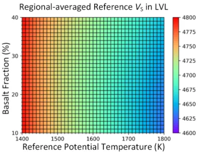
temperature. Figure 3 presents the predictions of regional-‐average shear wave speeds 214
for a range of potential temperatures and basalt fractions at a constant pressure of 215
11.7 GPa. The thermal and compositional effects can trade off with each other and 216
thus different combinations of the two variables may lead to the same velocities. 217
218
219
Figure 3 A heatmap showing the predicted regional-‐averaged reference shear wave velocities at
220
11.7 GPa in response to different combinations of reference potential temperature and basalt
221
fraction in the LVL beneath the western US
222 223
3.2 Partial melting and velocity reductions
224
To simulate the influence of partial melting on seismic velocities, we employ the 225
modelling scheme of Takei (2002), where the shear wave speed variation 𝜉 is governed 226
by the effective elastic moduli of the aggregate: 227
𝜉 = 𝑁/𝜇
𝜌 𝜌! (4)
, where 𝑁 is the elastic modulus of the intergranular skeletal framework that indicates 228
the strength of contact between the neighbouring grains; 𝜇 is the shear modulus; 𝜌! is
229
the density of the solid bulk; and 𝜌 is the volume-‐averaged density of the entire 230
aggregate which is calculated as: 231
, where 𝜌! is the density of the melt; 𝜑 is the volume fraction of melt within the
232
aggregate. 233
In eq. 4, the elastic modulus 𝑁 is determined by both the melt volume fraction 𝜑 234
and the contiguity (𝜓, i.e. the area fraction of the intergranular contact) of the melt: 235
𝑁 = 𝜇 1 − 𝜑 1 − 1 − 𝜓 ! (6)
The contiguity 𝜓 depends on the melt volume fraction 𝜑 and the dihedral angle 𝜃 236
between the solid grains and the melt; and 𝑛 is an exponent also depending on 𝜓 237
(Takei, 2002). The simulations of contiguity applied here are based on the micro-‐ 238
structural model of von Bargen and Waff (1986) which formulates the contiguity 𝜓 as 239
the proportion that the contact area of grains occupy among the total contact area in a 240
partial molten aggregate: 241
𝜓 = 2𝐴!!
2𝐴!!+ 𝐴!" (7) , where 𝐴!! and 𝐴!" are the grain-‐grain contact area and grain-‐melt contact area per
242
unit volume, respectively. The values of 𝐴!! and 𝐴!" are calculated from the given
243
melt volume fraction and dihedral angle using polynomial functions: 244
𝐴!! = 𝜋 − 𝑏!!power 𝜑, 𝑝!!
𝐴!" = 𝑏!"power 𝜑, 𝑝!" (8) The required constants 𝑏!!, 𝑏!", 𝑝!! and 𝑝!" are approximated from quadratic
245
polynomials of the dihedral angle (in degree), of which the values are outlined in von
246
Bargen and Waff (1986). Wimert and Hier-‐Majumder (2012) indicated this 247
approximation of contiguities can produce satisfactory fits with experimental 248
measurements from partially molten aggregates with melt volume fractions below 5%. 249
Combining equations 3—7 enables the contiguity to be expressed as a function of 250
the melt volume fraction 𝜑 and dihedral angle 𝜃, i.e. 𝜓 = 𝜓 𝜑, 𝜃 . Moreover, shear 251
wave speed anomalies 𝜉 caused by partial melting can be formulated as a function 252
with respect to melt volume fraction and dihedral angle: 253
𝜉 𝜑, 𝜃 = 1 − 𝜑 1 − 1 − 𝜓 𝜑, 𝜃
!
1 − 𝜑 1 − 𝜌! 𝜌! (9)
We estimate the densities of solid bulk 𝜌! and melt 𝜌! using the third-‐order Birch-‐
254
Murnaghan equation of state (EOS), as Ghosh et al. (2007) suggested for carbonated 255
peridotite melt. We implement the mathematic approximations using a Python 256
computational toolkit for microscale geodynamic study, named as Multiphase Material 257
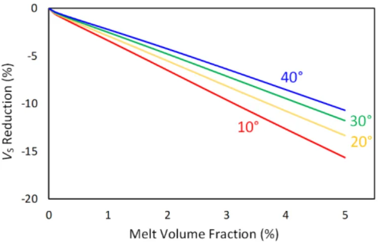
Properties forward model (MuMaP, Hier-‐Majumder, 2017). The modelled shear wave 258
velocity reductions (in percentage) in response to a variety of melt volume fractions 259
and dihedral angles are illustrated in fig. 4. Each of the curves in the cross-‐plot 260
represents the shear wave velocity reductions caused by the melt with volume 261
fractions from 0 to 5% at a fixed dihedral angle, showing that the velocity in the 262
partially molten aggregates decreases rapidly as the fraction of melt increases. The 263
upward shifting of the curves indicates that, for the same melt volume fraction, a 264
smaller dihedral angle can result in greater reductions in the shear wave speed. 265
However, different combinations of dihedral angles and melt volume fractions may 266
produce the same extent of shear-‐velocity reduction. 267
268
Figure 4 Predicted shear wave velocity reductions for different melt volume fractions and dihedral
269
angles. The corresponding dihedral angles to the curves are annotated on the plot. Each curve
270
shows the velocity reductions caused by changes in melt volume fraction at a fixed dihedral angle
271 272
4 Model inversion 273
The forward modelling approach described in the preceding section predicts the 274
shear wave velocity reductions in response to associated parameters. Alternatively, if 275
seismic data of the LVL are available, it is possible to calculate the velocity reductions 276
as a ratio of the observed velocity over the reference velocities: 277 𝜉 = 𝑉! !"# 𝑉!!"# 𝑇 !, 𝐶 (10) When embedded with an inversion scheme, the numerical model can be used to 278
deduce the multiple controls on seismic velocities. The inversion procedure can begin 279
with an initial solution that is built upon petrologic and seismological constraints. We 280
then investigate how to exploit and utilize the symmetry of the model, which can allow 281
us to alter the initial solution directly into another solution whilst giving the same 282
observations. In this way, the additional solutions to the inverse problem can be 283
rapidly derived by repetitively use of the transformation. 284
285
4.1 An initial solution based on a priori knowledge
286
To incorporate the forward model and the observed data in a single framework, 287
we firstly combine eq. 9 and 10: 288 1 − 𝜑 ∙ 1 − 1 − 𝜓 𝜑, 𝜃 ! 1 − 𝜑 1 − 𝜌! 𝜌! = 𝑉!!"# 𝑉!!"# 𝑇 !, 𝐶 (11)
, which gives four unknowns (i.e. 𝑇!, 𝐶, 𝜃 and 𝜑) in one equation. To solve melt volume
289
fraction 𝜑 from the eq. 11, the reference potential temperature 𝑇!, basalt fraction 𝐶
290
and dihedral angle 𝜃 need to be specified. We initially assume the reference potential 291
temperature to be 1500 K in the region. We set the basalt fraction at 18%, as 292
suggested in Xu et al. (2008) for common peridotite. The dihedral angle at the grain-‐ 293
melt interface varies with the chemical composition of the melt. For example, Minarik
294
and Watson (1995) proposed dihedral angles varying from 25 to 30° at the interface 295
between carbonate melt and molten aggregates; Mei et al. (2002) suggested a dihedral 296
angle of 28° for molten aggregates with hydrous basalt melt. Here we initially assume a 297
dihedral angle of 𝜃 = 25°. Given these a priori assumptions, 𝑇!, 𝐶 and 𝜃 are specified,
298
and hence the melt volume fraction can be solved from eq. 11. 299
We then calculate the corresponding melt volume fraction 𝜑 using a modified 300
Newton-‐Raphson root-‐search algorithm (Press et al., 2007, chap. 9.1), same as the 301
calculation in Hier-‐Majumder and Tauzin (2017). The algorithm begins with a bracket 302
for the melt volume fraction between 1×10-‐4% and 10% and iterates the searching
303
process until a convergence of 10-‐4% is achieved in the inferred fraction. Figure 5
304
shows the initial solution derived from the inversion using the seismic observations 305
and the constraints on 𝑇!, 𝐶 and 𝜃. The melt fractions in the region vary spatially and
306
yields an average of 0.72%. The synthetic velocities reproduced from the forward 307
model (fig. 5c) proves a good match to the real observations (fig. 1d). 308
309
310
Figure 5 An initial solution found from the inverse problem. The observed shear wave velocities (a)
311
and reference values of 𝑇!, 𝐶 and 𝜃 are used to provide constraints on the inversion. A particular
312
inference of the melt vol. % within the LVL (b) is then generated using a root-‐search approach. The
313
regionally averaged fraction is calculated as 0.72% given 𝑇! = 1500 K, 𝐶 = 18% and 𝜃 = 25°. Using
314
the inferred melt vol. % and the reference values, shear wave velocities (c) can be reproduced from
315
the forward model
4.2 Symmetric transformation
317
The above calculation generates a single solution to the inverse problem. Since the 318
inverse problem is non-‐unique with respect to the input parameters 𝑇!, 𝐶 and 𝜃, there
319
are, in principle, an infinite number of alternative solutions that can reproduce 320
identical seismic observations. Here we develop a quantitative approach to prove the 321
non-‐uniqueness and, more crucially, the transformation from an existing solution to an 322
alternative solution. The symmetry of the numerical model is found by properly 323
modifying the input parameters to obtain an unchanged output model. To start with, 324
we formulate the forward model of shear wave speed as: 325
𝑽! = 𝐹 𝑇!, 𝐶, 𝜃, 𝝋 (12)
, where 𝑽! is the shear wave speeds in the LVL beneath the seismic sites; 𝐹 denotes a
326
general, non-‐linear function (in this work, 𝐹 is the forward model from the code 327
MuMaP_fwd) and 𝝋 is a vector of melt volume fractions in the LVL. Note that 583 328
seismic sites are analysed in this study, and hence the vector lengths are 583 for both 329
𝑽! and 𝝋. We then generate three perturbations 𝛿𝑇!, 𝛿𝐶 and 𝛿𝜃 respectively into the
330
three variables 𝑇!, 𝐶 and 𝜃. These small changes in the model inputs thus give rise to
331
residuals in the modelled velocities, i.e. ∆𝑽!. This can be written as:
332
∆𝑽! = 𝐹 𝑇! + 𝛿𝑇!, 𝐶 + 𝛿𝐶, 𝜃 + 𝛿𝜃, 𝝋 − 𝐹 𝑇!, 𝐶, 𝜃, 𝝋 (13)
, which may be approximated in a linear form using the first-‐order Taylor’s series: 333 𝜕𝐹 𝜕𝑇!𝛿𝑇!+ 𝜕𝐹 𝜕𝐶𝛿𝐶 + 𝜕𝐹 𝜕𝜃𝛿𝜃 = ∆𝑽! (14)
, where 𝜕𝐹/𝜕𝑇!, 𝜕𝐹/𝜕𝐶 and 𝜕𝐹/𝜕𝜃 are finite derivatives of the function 𝐹 with
334
respect to 𝑇!, 𝐶 and 𝜃. We then calculate changes required in the melt volume
335
fractions (i.e. 𝛿𝝋) to compensate the changes in velocities resulting from the 336
perturbations. This can be expressed as: 337
𝐹 𝑇!+ 𝛿𝑇!, 𝐶 + 𝛿𝐶, 𝜃 + 𝛿𝜃, 𝝋 + 𝛿𝝋 − 𝐹 𝑇!, 𝐶, 𝜃, 𝝋 = 𝟎 (15)
Approximation based on the Taylor’s series gives: 338 𝜕𝐹 𝜕𝑇!𝛿𝑇!+ 𝜕𝐹 𝜕𝐶𝛿𝐶 + 𝜕𝐹 𝜕𝜃𝛿𝜃 + 𝜕𝐹 𝜕𝝋𝛿𝝋 = 𝟎 (16)
, where 𝜕𝐹/𝜕𝝋 is the finite derivative of the function 𝐹 with respect to 𝝋. We then 339
solve 𝛿𝝋 by combining eq. 14 and 16: 340
𝛿𝝋 = − ∆𝑽𝐒
𝜕𝐹/𝜕𝝋 (17)
In this equation, 𝜕𝐹/𝜕𝝋 can be calculated from the forward model. We make small 341
changes in 𝝋 and then run the model to predict the corresponding velocities. The 342
values of 𝜕𝐹/𝜕𝝋 are given by the difference in the modelling outputs divided by the 343
small changes in 𝝋. Note that 𝛿𝝋, 𝜕𝐹/𝜕𝝋 and ∆𝑽! are all vectors with a length of 583
344
as there are 583 locations in total. Given the perturbations 𝛿𝑇!, 𝛿𝐶 and 𝛿𝜃 and the
345
required adjustments in melt volume fractions 𝛿𝝋, the model 𝐹 𝑇!+ 𝛿𝑇!, 𝐶 + 𝛿𝐶, 𝜃 +
346
𝛿𝜃, 𝝋 + 𝛿𝝋 can produce the same shear wave speeds as given by the initial solution. 347
The new solution can then be used as a basis for another transformation. Iterative 348
transformation can therefore derive all the additional solutions to the inverse problem. 349
350
4.3 Calculating multiple solutions
351
Using the forward model and symmetric transformation, we then examine the 352
entire parameter space and calculate alternative solutions. The parameter space can 353
be considered as a 3-‐D volume of which the three dimensions are potential 354
temperature (𝑇!), basalt fraction (𝐶) and dihedral angle (𝜃). We define the ranges of
355
the parameters as 1400 to 1800 K in potential temperature, 10 to 40% in basalt 356
fraction and 10° to 40° in dihedral angle. We also set the increments at 10 K in 357
potential temperature, 1% in basalt fraction and 1° in dihedral angle. Therefore, the 358
parameter space is finely sampled and thus the transformation approach can apply. 359
Each position in the parameter space can be described using the coordinates in the 360
three dimensions. If a solution exists in position 𝑇!, 𝐶, 𝜃 , then the corresponding melt
361
volume fraction vector can be written as 𝝋 𝑇!, 𝐶, 𝜃 . Once a solution is found, the
362
solutions in neighbouring positions can also be determined. Because the 363
transformation can be applied both forward and backward, six neighbouring solutions 364
should be examined, including 𝝋 𝑇!+ 𝛿𝑇!, 𝐶, 𝜃 , 𝝋 𝑇!− 𝛿𝑇!, 𝐶, 𝜃 , 𝝋 𝑇!, 𝐶 + 𝛿𝐶, 𝜃 ,
365
𝝋 𝑇!, 𝐶 − 𝛿𝐶, 𝜃 , 𝝋 𝑇!, 𝐶, 𝜃 + 𝛿𝜃 and 𝝋 𝑇!, 𝐶, 𝜃 − 𝛿𝜃 . We calculate the additional
366
solutions through the following procedure: 367
(1) Create an empty list. Add the coordinate of the initial solution into the list. 368
(2) For each solution in the list, calculate the solutions in the neighbouring 369
positions that are inside of the parameter space but not existing in the list. 370
(3) Add the solutions found in step (2) into the list. 371
(4) Return to step (2) and repeat the workflow until no new solution can be 372
added into the list. 373
Note that this is different from a brute-‐force search which involves a root-‐ 374
searching approach for calculating the melt volume fraction beneath every location 375
given different combinations of 𝑇!, 𝐶 and 𝜃. In contrast, the symmetric transformation
376
is straightforward as it can simultaneously derive the melt volume fraction beneath the 377
whole area. Since this method works directly on the behaviour of the solution with 378
respect to perturbations, it also allows us to predict regions where solution does not 379
exist and the solution containing the lowest possible average melt fractions, which was 380
intractable with the method described by Hier-‐Majumder et al. (2014). 381
382
4.4 Complete solutions to the inverse problem
383
Using the above computational procedure, we derive all the solutions in the 384
parameter space. All the possible solutions can reproduce the same synthetic shear 385
wave velocities from the forward model. Significant spatial variations in the inverted 386
melt volume are found in every solution. Because the melt volume fraction should 387
always be non-‐negative, the calculated vectors of 𝝋 where one or more negative 388
values exist should be removed. Given this requirement, limits can be placed to bound 389
the symmetric transformation, i.e. not every combination of potential temperatures, 390
basalt fractions and dihedral angles in the parameter space is compatible with the 391
seismic observations, though not a unique solution to the inverse problem can be 392
found. Example of the variations in calculated melt volume fractions and the 393
transformation limits in the multiple controlling factors are demonstrated in fig. 6. 394
395
Figure 6 Series of box-‐plots showing the estimated melt vol.% beneath all locations with median
396
indicated by the horizontal line within each box, upper/lower quartiles indicated by the
397
upper/lower edges of the box and maximum/minimum indicated by whiskers of the boxes. (a) & (b)
398
Inferred melt vol.% as a function of reference potential temperature with fixed basalt fraction and
399
dihedral angles. (c) & (d) Inferred melt vol.% as a function of basalt fractions with fixed reference
400
potential temperature and dihedral angle. (e) & (f) Inferred melt vol.% as a function of dihedral
401
angle with fixed reference potential temperature and basalt fractions. Note that no solution can be
402
found given 𝑇! ≥ 1500 in (a), 𝑇! ≥ 1550 K in (b) and 𝐶 ≤ 30% in (d)
403 404
The model output illustrated in fig. 7 is an end-‐member solution showing that the 405
lowest possible averaged melt volume fraction is 0.51%, associated with 𝑇! = 1550 K, 𝐶
406
= 40% and 𝜃 = 10°. In this solution, the melting is not predicted beneath some regions, 407
for instance at the triple border between Idaho, Montana and Wyoming. Considering 408
the sharp boundary atop the LVL, this may just be an artefact because the variations in 409
solid bulk are unlikely to produce the rapid velocity reductions. However, this solution 410
is still meaningful since it places a lower-‐bound below the regional-‐averaged melt 411
volume fraction within the observed LVL. In contrast, the highest possible averaged 412
melt volume fraction that exists in the parameter space yields 1.47%, associated with 413
𝑇! = 1400 K, basalt fraction 𝐶 = 10% and dihedral angel 𝜃 = 10°, as shown in fig. 8. 414
Examples of the trade-‐offs between the estimated melt volume fraction below a given 415
location and the multiple controls are displayed in fig. 9 by cross-‐plotting the estimates 416
and the corresponding controlling factors. Whilst the forward model used here is non-‐ 417
linear, application of the proposed method has indicated the trajectories that link 418
together the multiple solutions in the parameter space. 419
421
Figure 7 The end-‐member solution with the minimum melt vol. % within the LVL beneath the w.
422
The regional averaged melt vol. % is 0.51% given 𝑇! = 1550 K, 𝐶 = 40% and 𝜃 = 10°. Note that this
423
solution is directly derived from the initial solution, rather than from a brute-‐force search
424 425
426
Figure 8 The end-‐member solution with the maximum melt vol. % within the LVL beneath the
427
region. The regional averaged melt vol. % is 1.47% given 𝑇! = 1400 K, 𝐶 = 10% and 𝜃 = 40°. Note
428
that this solution is directly derived from the initial solution, rather than from a brute-‐force search
430
Figure 9 Cross-‐plots of inferred melt volume fraction beneath 106°W, 35°N (label A in fig. 1a)
431
versus (a) the reference potential temperature for different dihedral angles ranging from 10° to 40°
432
(annotated on the plot) with constant intervals of 5° given a fixed basalt composition and (b) the
433
basalt fraction in the bulk composition for a range of different dihedral angles given a fixed
434 potential temperature 435 436 5 Discussion 437
Using a numerical inversion approach, we have examined the LVL at 350 km 438
underneath the western US. The shear-‐velocity anomalies and impedance contrasts in 439
this zone have been thought to indicate a small fraction of volatile-‐rich melt (Hier-‐
440
Majumder and Tauzin, 2017) released either by the decarbonation during the Farallon 441
slab subduction (Thomson et al., 2016) or by the dehydration from the upwelling of 442
the Yellowstone mantle plume or small-‐scale convection within the MTZ (Bercovici and
443
Karato, 2003; Richard and Bercovici, 2009; Zhang et al., 2018). Despite the presence of 444
petrological and geochemical evidences of melting near the MTZ, determination of the 445
quantity of melting from seismic signatures remains hard work owing to the trade-‐offs 446
that exist between various controlling factors. Due to the lack of geophysical and 447
geochemical constraints, it is difficult, if not impossible, to distinguish the individual 448
effects of temperature, composition and partial melting. A recent study has further 449
suggested that these multiple controls are strongly correlated, leading to a 450
disagreement between the experimental measurements and theoretical estimates 451
(Freitas et al., 2019). 452
Our numerical scheme based on a symmetry is able to cover all solutions. Using a 453
forward model, we firstly generate an arbitrary solution assuming 𝑇! = 1500 K, 𝐶 = 18%
454
and 𝜃 = 25°. This is a successful solution as the shear wave velocities it predicts are 455
consistent with the observations. The inverse problem is then linearized to find 456
neighbouring solutions to the initial solution. As the controlling parameters have only a 457
limited range of plausible values (in this work 1400 ≤ T0 ≤ 1800 K, 10% ≤ C ≤ 40% and 458
10° ≤ θ ≤ 40°), the symmetry gives a quasi-‐complete set of solutions subject to the 459
necessary constraint that the melt volume fraction in the upper mantle must always be 460
non-‐negative. This constraint can be justified as the effects of temperature and 461
composition are already taken into account. Given the above treatment, it is then a 462
simple matter to find the combinations of parameters that reveals the end-‐member 463
possibilities (e.g. maximum and minimum degrees of partial melting). 464
The modelling results show that a regional-‐averaged melt volume fraction of 465
approximately 0.51% is necessary to explain the sharp shear-‐velocity reductions at 350 466
km beneath the western US. This is the minimum extent of melting required to 467
produce the observed LVL, whatever the solid mantle conditions and the geometry of 468
the melt are. As Hier-‐Majumder and Courtier (2011) suggested, at such a small level of 469
melting, a near neutrally buoyant melt can migrate over the LVL due to surface 470
tension, whereas the drainage efficiency of both buoyant and dense melts is likely 471
insignificant. 472
As no solution has been found to be associated with a reference potential 473
temperature higher than 1550 K, we can place an upper-‐bound on the variations in the 474
reference potential temperature. The modelling output also shows that the range of 475
variations in basalt fraction depends on the assumed reference potential temperature. 476
At a low reference potential temperature (e.g. 1400 K), the basalt fraction may vary 477
from 10% to 40%. In contrast, at a higher reference potential temperature, solutions 478
can only be in the basaltic-‐rich zone (e.g. fig. 6d). For instance, Hier-‐Majumder and
479
Tauzin (2017) estimated the reference potential temperature as approximately 1550 K. 480
If this is the case, then we can make a statement that the basalt fraction in the LVL 481
beneath the western US is no less than 40%. Hence, whilst the thermal and 482
compositional conditions are still under-‐constrained, our model work offers more 483
reliable information about the mantle physical properties. 484
In addition, our inverse method unravels trade-‐offs between parameters. As the 485
forward model is non-‐linear, there is no simple analytical tool for determining these 486
competing effects. The numerical approach proposed here allows estimating the rates 487
of change in the inferred melt volume fraction caused by changes in other parameters. 488
According to the modelling outputs, the significance of the trade-‐offs between inferred 489
melt volume fractions and other parameters can be summarized as: 490
(1) For a given dihedral angle and a given basalt fraction, the inferred melt 491
volume fractions present a strong negative correlation with the assumed 492
reference potential temperatures (fig. 6a & b). 493
(2) For a given reference potential temperature and a given dihedral angle, the 494
inferred melt volume fractions are insensitive to the assumed basalt fractions 495
(fig. 6c & d). 496
(3) For a given reference potential temperature and a given basalt fraction, the 497
inferred melt volume fractions present a modest positive correlation with the 498
assumed dihedral angles (fig. 6e & f). 499
In this analysis, a number of assumptions are made about the mantle: it is in a 500
state of chemical disequilibrium (described as a mechanical mixture of basalt and 501
harzburgite), melt films are not playing a role in velocity reduction, the transition zone 502
thickness reflects temperature variations, the Clapyron slope is known, and receiver 503
function estimates of MTZ thickness are accurate. 504
This study calculates the temperature variations from the thickness of the MTZ 505
using the empirical correlation proposed by Tauzin and Ricard (2014). The empirical 506
model relies on several assumptions, for example that only temperature varies MTZ 507
thickness and that no vertical variation occurs in temperature from the MTZ to the LVL. 508
As observed from tomographic models (with low vertical resolution), the MTZ has 509
consistent structures over the whole range of depth, in particular the stalled Juan de 510
Fuca/Farallon slab (Burdick et al., 2008; Schmandt et al., 2011; Hier-‐Majumder and
511
Tauzin, 2017). Although an entirely consistent MTZ should not be expected, dealing 512
with the absolute topography of discontinuities to infer the temperatures would likely 513
introduce more uncertainties, as would require a precise correction of the effect of 514