Adjoint sensitivity analysis of the atmospheric impacts of combustion emissions

Adjoint sensitivity analysis of the atmospheric impacts

of combustion emissions

by

Irene Constantina Dedoussi

B.A., M.Eng., University of Cambridge (2012)

S.M., Massachusetts Institute of Technology (2014)

Submitted to the Department of Aeronautics and Astronautics

in partial fulfillment of the requirements for the degree of

Doctor of Philosophy in Aeronautics and Astronautics

at the

MASSACHUSETTS INSTITUTE OF TECHNOLOGY

June 2018

Massachusetts Institute of Technology 2018. All rights reserved.

Signature redacted

Author ...

re acted

Department of Aeronautics and Astronautics

AA .

May 2018

Signature redacted

Certified by ...

/ Stiven R.H. Barrett

Associate Professor of Aeronautics and Astronautics

Chair, Thesis Committee

Certifiedby...

Signature redacted

Susan Solomon

Lee and Geraldine Martin Professor of Environmental Studies

Member, Thesis Committee

Certified

by

...

Signature redacted

Daven K. Henze

Associate Professor of Mechanical Engineering

University of Colorado Boulder

Member, Thesis Committee

Accepted by

...

Signature redacted

MASSACHUSETTS INSTITUTE

Hamsa Balakrishnan

OF TECHNOLOGY

_{Associate Professor of Aeronautics and Astronautics}

Adjoint sensitivity analysis of the atmospheric impacts of

combustion emissions

by

Irene Constantina Dedoussi

Submitted to the Department of Aeronautics and Astronautics on May 25, 2018, in partial fulfillment of the

requirements for the degree of

Doctor of Philosophy in Aeronautics and Astronautics

Abstract

Combustion emissions impact the environment through chemical and transport processes that span varying temporal and spatial scales. Numerical simulation of the effects of com-bustion emissions and potential corresponding mitigation approaches is computationally expensive. Atmospheric adjoint modeling enables the calculation of receptor-oriented sensitivities of environmental metrics of interest to emissions, overcoming the numer-ical cost of conventional modeling. This thesis applies and further develops an existing adjoint of a chemistry-transport model to perform three evaluations, where the high num-ber of inputs (due to the nature of the problem or the associated uncertainty) prevented comprehensive assessment in the past.

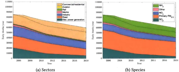
First, this thesis quantifies the pollution exchange between the US states for seven major anthropogenic combustion emissions sectors: electric power generation, industry, commercial/residential, aviation, as well as road, marine, and rail transportation. This thesis presents the state-level fine particulate matter (PM2.5) early death impacts of

com-bustion emissions in the US for 2005, 2011 and 2018 (forecast), and how these are driven

by sector, chemical species, and location of emission. Results indicate major shifts in the

chemical species and sectors that cause most early deaths, and opportunities for further improving air quality in the US.

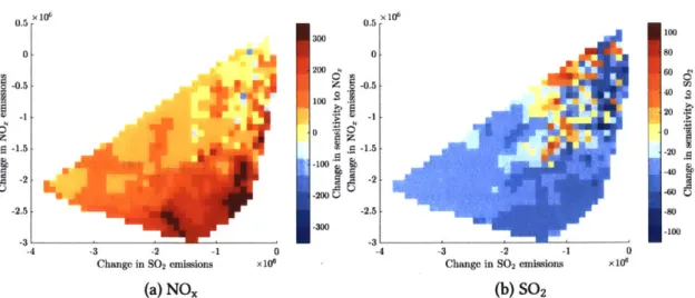
Second, this thesis quantifies how changes in emissions impact the marginal atmo-spheric PM2.5 response to emissions perturbations. State-level annual adjoint sensitivities

of PM2.5 population exposure to precursor emissions are compared for the years of 2006

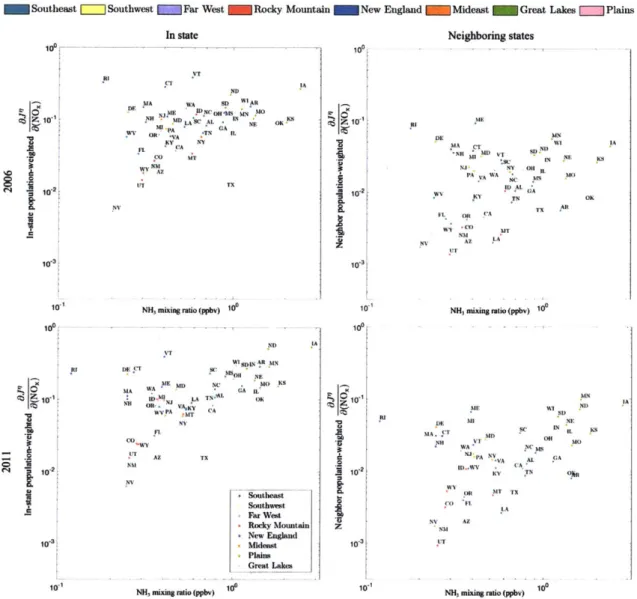
and 2011, and correlated with the magnitude of emissions reduction and the background ammonia mixing ratio.

the GEOS-Chem unified tropospheric-stratospheric chemistry extension (UCX), which enables the calculation of stratospheric sensitivities and the examination of the entire design space of high altitude emissions impacts. To illustrate its potential, sensitivities of stratospheric ozone to precursor species are calculated. This development expands the span of atmospheric chemistry-transport questions (including inversions) that this open-source model can be used to answer.

The assessments performed in this thesis span spatial scales from the regional to the global and demonstrate the ability of this approach to provide information on both bottom-up and top-down mitigation approaches.

Doctoral Committee Chair: Steven R.H. Barrett

Title: Associate Professor of Aeronautics and Astronautics

Doctoral Committee Member: Susan Solomon Title: Professor of Environmental Studies

Doctoral Committee Member: Daven K. Henze

Acknowledgments

The PhD journey, of which this thesis is a product, had several by-products, which, as is the case with combustion, end up mattering a lot. This is my attempted segue to men-tioning how retrospectively grateful I am for these by-products. Trying to look back, it is difficult doing justice to the people who deserve to be thanked over the years, but I will try my best in just a few paragraphs.

I would first like to thank my advisor, Prof. Steven Barrett, for giving me the

opportu-nity to work on exciting projects, and helping me become a better researcher and a better communicator. His ability to find solutions to all imaginable problems (academic and oth-erwise) is truly admirable. I am grateful to my PhD committee members, Prof. Susan Solomon and Prof. Daven Henze, who provided their experienced guidance and feedback in this work. I would like to thank Prof. Solomon for the stratospheric ozone discussions and for urging me to take the best class I've taken at MIT. I owe Prof. Henze for many discussions on the adjoint method, for being a great educator, and for the hospitality in Boulder. I would also like to thank Prof. John Hansman and Dr Seb Eastham whose help was valuable in improving the quality of this document.

I sincerely thank the MIT Martin Family Fellowship for Sustainability, the MIT ODGE

George and Marie Vergottis Fellowship, NASA project NNX14AT22A, and EPA project

RD-83587201, for funding me and various parts of this thesis. I owe to Mel, Anna, Beth,

and Jennie, who always cared, helped, and made convoluted tasks seem simple.

I want to thank the friends and colleagues at the Laboratory for Aviation and the

En-vironment (LAE) over the years, for the laughs, the conversations, and the collaborations. Many thanks in particular go to LAE veterans: to Akshay Ashok for teaching me more about planes than I'd ever wished to know; to Philip Wolfe for being capable of answer-ing literally every question I ever asked him; to Chris Gilmore for his calm and reasonable

presence; to Fabio Caiazzo for always checking in. Thanks to Ray, who dealt with my per-petual server storage requests without few complaints, and again to Seb for writing the

UCX and making my life more complicated. Thanks also go to Robert and Florian, for

adding a German note to what would have otherwise been a disorganized lab. Finally, thanks to Akshat for never saying no to a break, to Carla for being wonderful, and to L. Kulik for always disagreeing.

I've been lucky to have been surrounded by great friends who tolerated me at different phases. I'd like to thank Philip(o) for being an exemplar of a human being, eh!; Dan for providing beverages, distractions, and HMS SysBio hospitality; Lawrence for listening; the Greek Georges for the Miracle evenings; Kat for existing in the AeroAstro department; Liszl6 for moving far away; and Kendall for immersing me into the Southern ways.

R6mi probably deserves an entire paragraph in this, but will have to settle for a sen-tence. I'd like to thank him for doing his PhD with me, and for having lunch/coffee/cookie breaks on an un-restrictive basis. Thanks to David and Seb who (rumor has it) were also around MIT. A big thanks goes to the rest of Festivus for setting the fun bar way too high over the first two years, and for reuniting regularly to run 200 miles in a forest, boogieboard in Hawaii, or feel old at ACL.

I would also like to thank a series of non-US friends in Greece, the UK and Cyprus (Katerina, Maki (not the sushi), Priya, George, Oli, the 'Vouliagmeni girls', and many others), for staying friends with me during this PhD - I'm sure that was a lot of effort on their end. They, together with my family (pappous Kotsos, Lila, Kostas, and others), always made sure I felt involved, even when being very far away.

A special thanks goes to Parth, who practically witnessed and endured, live or

re-motely, this PhD.

Finally, and most importantly, thank you to my parents, Stella and Vassilis, and my brother Dimitris. There are not enough words to describe their importance through all this. This thesis (and many other things in my life) is because of them.

Contents

1 Introduction 15

1.1 Adjoint method . . . . 15

1.1.1 Adjoint theory . . . . 15

1.1.2 Adjoint applications in atmospheric science . . . . 18

1.1.3 Source-attribution alternatives . . . . 21

1.2 US air quality . . . . 23

1.3 Emissions in the stratosphere . . . . 27

1.4 Thesis contributions . . . . 29

1.5 Thesis outline . . . . 31

2 Pollution exchange between the US states 33 2.1 Introduction . . . . 33

2.2 Methods . . . . 36

2.2.1 Sectoral emissions . . . . 37

2.2.2 Air quality modeling . . . . 38

2.2.3 Impacts assessment . . . . 40

2.2.4 Health impacts . . . . 40

2.3 R esults . . . . 42

2.3.2 Sectoral and speciated attribution . . . . 42

2.3.3 Pollution exchange between the states . . . . 45

2.3.4 Policy implications . . . . 48

2.4 Discussion and conclusions . . . . 48

3 State-level changes of PM2.5 population exposure sensitivities to emission precursors 51 3.1 Introduction . . . . 52 3.2 Methods . . . . 54 3.2.1 Emissions . . . . 55 3.2.2 Adjoint sensitivities . . . . 55 3.3 Results . . . . 56

3.3.1 Aggregate US sensitivity changes . . . . 56

3.3.2 State-level sensitivity changes . . . . 60

3.3.3 Ammonia dependence . . . . 61

3.3.4 Policy implications . . . . 62

3.4 Discussion and conclusions . . . . 66

4 Development of the adjoint of the GEOS-Chem unified chemistry exten-sion 69 4.1 Introduction . . . . 70

4.2 Methods . . . . 71

4.2.1 The GEOS-Chem UCX model . . . . 72

4.2.2 Adjoint model development . . . . 73

4.3 Results . . . . 74

4.3.1 Model evaluation . . . . 74

4.4 Discussion and conclusions... ... . . .. .. ... .... 8

5 Conclusions 87 5.1 Summary of findings and contributions . . . . 88

5.2 Lim itations . . . . 90

5.3 Recommendations for future work . . . . 91

5.3.1 Regional near-surface air quality . . . . 92

5.3.2 Adjoint of the GEOS-Chem UCX model . . . . 95

A Source-receptor relationships 99

B Regional definitions 115

C Additional sensitivity changes results 117

D GEOS-Chem UCX adjoint development specifics 123

List of Figures

2-1 Cross-state impacts approach schematic . . . 36

2-2 Total annual early deaths attributable to each sector and each species be-tween 2005 and 2018 . . . . 43

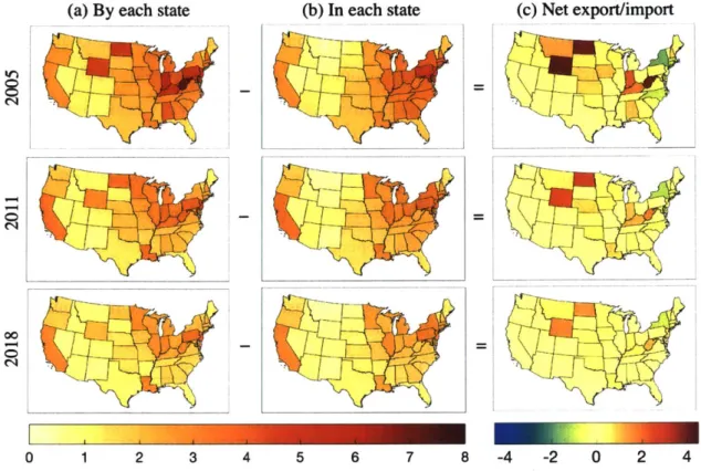
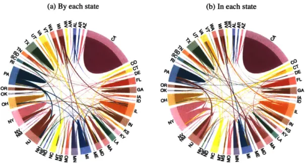
2-3 Total annual early deaths caused per 10,000 people for 2005, 2011 and 2018. 45 2-4 Cross-state exchange of annual early deaths for 2018. . . . . 47

3-1 Sensitivity changes approach schematic . . . . 54

3-2 US population PM2.5 exposure sensitivities to NOx and SO2 emissions per-turbations . . . . 57

3-3 Changes in atmospheric response to NOx and SO2 emissions, given changes in NOx and SO2 emissions . . . . 59

3-4 Relative changes in NOx and SO2 emissions and PM2.5 adjoint sensitivities in each state between 2006 and 2011 . . . . 64

3-5 Population weighted state-level PM2.5 adjoint sensitivities against state-level NH3 mixing ratios . . . . 65

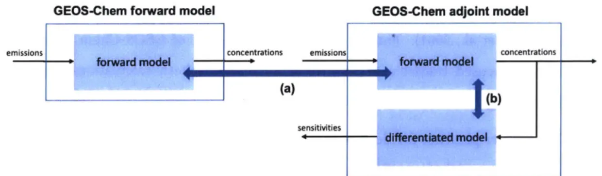
4-1 Model development and evaluation approach schematic . . . . 72

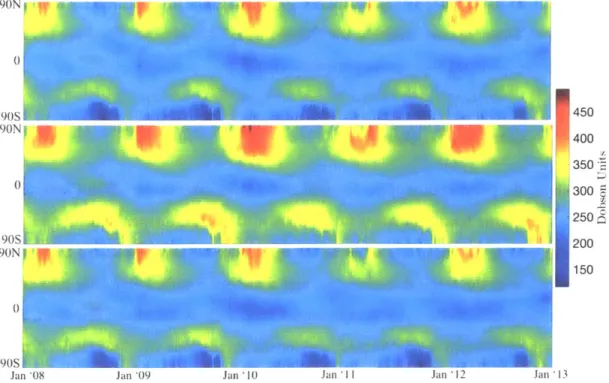
4-2 Zonal-mean column ozone model comparisons for 2008-2012 . . . . 76

4-3 Mean column ozone model comparisons for 2010 . . . . 77

4-5

4-6

Sensitivities of stratospheric

Ox

ClONO2 mixing ratios . . . .

4-7 Zonal sensitivities of aggregate Ox at a stratospheric altitude to BrO and

ClO mass perturbations . . . .

4-8 Zonal sensitivities of aggregate Ox at two altitude bands . . . .

A-1 Total annual early deaths maps for 2005, 2011 and 2018. . . A-2 West Virginia sources and receptors of health impacts . . . A-3 Wyoming sources and receptors of health impacts . . . . .

A-4 NY impacts' origins . . . .

A-5 NC impacts' origins . . . . A-6 IN emissions' impacts . . . . A-7 KY emissions' impacts . . . .

B-1 Definition of regions . . . .

C-1 US population PM2.5 exposure sensitivities to BC . . . .

C-2 CA and CO population PM2.5 exposure sensitivities to NOx

C-3 US gas ratio maps . . . .

. . . 102 . . . 103 . . . 104 . . . 105 . . . 106 . . . 107 . . . 108 . . . 115 . . . 117 and SO₂ . . . 118 . . . 119

C-4 Changes in atmospheric response to NOx and SO2 emissions, given changes

in NOx and SO2 emissions using an alternative filter . . . .

C-5 Relative changes in state-level PM2.5 adjoint sensitivities to out-of-state

em issions . . . .

C-6 Population weighted state-level PM2.5 adjoint sensitivities to SO2 against

state-level NH3 mixing ratios . . . .

D-1 Zonal-mean NOx for 2010 from the forward UCX model (left), the base

adjoint model (middle) and the base UCX adjoint model (right). . . . .

81 82 83 84 120 121 122 125

List of Tables

2.1 Summary of data used for each year . . . . 41

2.2 Primary PM2.5, NO, and SO, emissions totals... 42

2.3 States with the highest early death change . . . . 46

3.1 Annual anthropogenic emissions totals in the US for 2005 and 2011 . . . . 55

A.1 A.2 A.3 A.4 A.5 A.6 A.7 Early deaths attributable to each sector for 2005, 2011, and 2018 . . . 100

Early deaths attributable to each emission species for 2005, 2011, and 2018 101 Source-receptor matrix for 2005 - Total . . . 110

Source-receptor matrix for 2011 - Total . . . 111

Source-receptor matrix for 2018 - Total . . . 112

Source-receptor matrix for 2011 - Electric power generation . . . 113

Source-receptor matrix for 2011 - Road transporation . . . 114

D.1 UCX addition descriptions . . . . D.2 List of added tracers . . . . . . . 124

Chapter 1

Introduction

This thesis provides contributions in two themes: the US air quality impacts of combustion emissions and the stratospheric ozone impacts of high altitude emissions. The majority of this thesis employs the adjoint method to link impacts of interest directly to emissions. In this chapter, the adjoint method is described and its applications in atmospheric chem-istry are reviewed, along with alternative approaches. The two main themes of this thesis are then individually introduced and motivated. Finally, the thesis contributions are pre-sented.

1.1 Adjoint method

1.1.1

Adjoint theory

The word adjoint in mathematics means conjugate transpose. For a matrix with real en-tries its corresponding adjoint matrix is its transpose. Adjoint methods depend on this transpose matrix formulation, as will be explained below.

Let Y be the solution of a discretized partial differential equation or some other set of

P variables will be referred to as control variables. We wish to compute some function g(x,p) based on these parameters and the solution. Aside from the value of g, we also

want to know its gradient, d.

dg'~

This gradient of g with respect to 'can be useful as it gives the sensitivity of the quan-tity of interest with respect to the parameters . By appropriately defining the quanquan-tity of interest g, the sensitivities can be used to provide information regarding the impacts of uncertainty in the parameters A, and to optimize the parameters ' or the model itself.

An example will be provided here to demonstrate the basis of how the adjoint method is computationally efficient, as per Johnson (2012). Let the aforementioned X' be the solu-tion to the following linear equasolu-tion,

AY = b, (1.1)

where A is an M x M matrix and X is a column vector and the solution to the linear

equation. A and b depend on ' in some way. The gradient is calculated as follows:

dg og Og _(.

d- = (1.2)

dfi 01 OY ofi

gg + gig4, (1.3)

where the subscripts indicate partial derivatives. Given that g is a known and, depending on its definition, usually simple function, computing gg and gy is not a concern from a computational cost perspective. On the other hand, the computation of

4'

Xpi = A- (pi - A X) (1.4)

We would thus need to solve the M x M equation P number of times (once for every

component of p-). This is of significant computational cost if P and M are large. Overall we would need to calculate:

M x M1 9zxg = 9y A-' b$g - Ap (1.5) '1

M

Calculating gsx4 as per equation 1.5 involves multiplying an M x M matrix with an M x P matrix resulting in O(M2P) computation cost. However, if the calculation is

parenthesized in a different way (see eq. 1.6), we multiply a vector 1 x M with a M x P

matrix, and hence reduce the number of operations to O(MP). Solving for an adjoint equation entails changing the order of matrix-matrix and matrix-vector operations, and results in significant reduction in computational cost.

Although this example demonstrates the adjoint method in a simple algebraic equa-tion, the same principle applies to algorithms that integrate a set of equations in time (such as chemistry-transport models introduced below). In addition, however, the solu-tions 7 at every time step need to be stored, in order to perform the integration of the adjoint equation backwards in time, from time-step, t, to 0. Hence, one of the limitations of adjoint methods in time-dependent problems is the high memory storage requirement.

1.1.2

Adjoint applications in atmospheric science

The adjoint method allows the computation of gradients in a numerically efficient way. Adjoint operators can be derived for sets of equations that we normally refer to as models (Errico, 1997) and hence have a wide variety of potential applications, primarily in systems of ordinary or partial differential equations.

The adjoint method comes from optimal control theory (Lions, 1971) and has been applied in a viariety of fields including computational fluid dynamics (for e.g. aerodynamic design optimization (Jameson, 1988; Giles and Pierce, 2000)), quantum and nuclear reactor physics, oceanography, seismology, meteorology, etc. A comprehensive history of the adjoint method is provided by Marchuk et al. (2005) and Cacuci and Schlesinger (1994). In the field of earth sciences, the adjoint method was first applied in atmospheric science (Marchuk, 1974; Lamb et al., 1975), and then widely used in meteorology (Talagrand and Courtier, 1987; Errico and Vukicevic, 1992).

Chemistry-transport models (CTMs) simulate atmospheric chemical and physical pro-cesses in a Lagrangian or Eulerian manner. They have evolved from 2-D models with sim-plified chemistry, to full 3-D models, that simulate the transport, gas- and aerosol-phase chemistry and wet and dry deposition in the atmosphere. They are driven by assimi-lated meteorological data and emissions from a variety of inventories, and output species concentrations among other parameters of interest.

The adjoint method was first introduced in Lagrangian models (Fisher and Lary, 1995; Elbern et al., 1997). The first application of the adjoint method in an Eulerian CTM that included chemistry was by Elbern and Schmidt (1999). Since then, the adjoint method has been applied in a variety of regional and global CTMs, including but not limited to regional models CHIMERE (Vautard et al., 2000; Menut et al., 2000; Schmidt and Martin,

2003), Polair (Mallet and Sportisse, 2004, 2006), DRAIS (Nester and Panitz, 2006), STEM

and Henze, 2015), and global models IMAGES (Miller and Stavrakou, 2005; Stavrakou and Mler, 2006), and TM4 (Meirink et al., 2006). Hakami et al. (2007) developed the adjoint of US EPA's widely used regional CTM, the Community Multiscale Air Quality

(CMAQ). Henze et al. (2007) developed the adjoint of GEOS-Chem, the first adjoint of a

global CTM that included dynamics and extensive chemistry (full tropospheric chemistry, heterogeneous chemistry and aerosol thermodynamics).

In atmospheric science, adjoint models are widely used for inverse modeling, in par-ticular applied for remote sensing of atmospheric composition, generating top-down con-straints on surface fluxes, and chemical data assimilation (Brasseur and Jacob, 2017). Ex-amples include using gradient based optimization for refining the estimates of trace gases in the atmosphere (Kopacz et al., 2009, 2010, 2011; Wells et al., 2015; Bousserez et al., 2016; Paulot et al., 2014; Zhu et al., 2013; Jiang et al., 2017), improving the agreement of model predictions and insitu observations or remote sensing (Chai et al., 2006), as well as air quality forecasting (Kukkonen et al., 2012).

Besides inverse modeling, adjoint models are employed in sensitivity analyses. As explained by Hakami et al. (2007), sensitivity analysis can be performed in a forward or backward manner. In the forward method, sensitivities are propagated from the perturbed source into the various receptors/outputs. The methods in this category (one of which is finite-difference) are efficient in simultaneously providing information about all receptors with respect to the perturbed parameter. This method however is constrained by numeri-cal noise, and breaks down in model discontinuities. In the backward sensitivity analysis, a perturbation in the receptor is propagated backwards in time and space through an aux-iliary set of equations. As a result, the adjoint sensitivity analysis provides simultaneous sensitivity information about specific receptors with respect to all sources and parameters. The adjoint sensitivities are receptor-oriented, allowing us to attribute a scalar quan-tity of interest, also referred to as objective function, J, to emission species, emission location and time of emission (as well as other model parameters). Expressed as

OE(WZ~j~707(1.7) BE(,i,

j, k,

they can be used to quantify how a perturbation of emission, E, of species w, at location

(i,

j

They can thus be employed to assess the impacts of individual emissions changes (pertur-bations), such as policy scenarios, or the impacts of groups of emissions. The sensitivities provide the entire design space of possible emissions impacts as well as the possibility to quantify trade-offs between emissions reductions (e.g. Ashok et al. (2014)) and pinpoint optimal locations and times for emissions reductions for maximum benefits (e.g. Dedoussi and Barrett (2014)).

Adjoint sensitivity analysis has been employed to address questions that link emis-sions of various sectors to environmental and health metrics of interest. Koo et al. (2013) used the adjoint of GEOS-Chem to capture the intercontinental impacts of high-altitude emissions. Gilmore et al. (2013) quantified the contributions of individual flights to tro-pospheric ozone mass. Dedoussi and Barrett (2014) used the adjoint of GEOS-Chem to attribute the athropogenic emissions air quality impacts to location, time, species and sector. Turner et al. (2015) used the adjoint of the Community Multiscale Air Quality

(CMAQ) model for sectoral source apportionment of BC emissions impacts in the US. Lee

et al. (2015) used the adjoint of GEOS-Chem for source apportionment of global PM2.5

related mortality changes. Pappin et al. (2016) used the adjoint of CMAQ to estimate the public health benefits in the Canadian domain of reducing NOx emissions, on a per-ton and source-by-source basis. Kim et al. (2015) and Koplitz et al. (2016) performed a sensi-tivity study of health impacts from fires in Equatorial Asia.

1.1.3

Source-attribution alternatives

This thesis focuses on the adjoint method in terms of its source-attribution capabilities in a sensitivity analysis context. There are alternative ways of quantifying the relationship between source and receptor in an atmospheric chemistry and physics context, and these are summarized in this section. As previously described, the modeling approaches can be categorized into source-oriented and receptor-oriented. In a source-oriented approach, perturbations of individual model inputs are traced to a variety of different model outputs. In a receptor-oriented approach, perturbations of a variety of model inputs are traced to individual model outputs. The former is well-suited for characterizing how various outputs of interest (species, locations, times) are impacted by a limited number of changes in the model parameters. Source-oriented approaches are thus employed for example in cases where the model outputs of interest are significantly higher than the model inputs of interest. The latter, receptor-oriented approach is well-suited for characterizing how a specific number of model outputs is influenced by numerous model parameters. As previously mentioned this approach is applied in cases where the number of inputs of interest is significantly higher than the number of output quantities of interest. A review of the different approaches, including accuracy and uncertainty comparisons, is provided

by Cohan and Napelenok (2011).

Examples of source-oriented approaches include the following:

- Brute-force. This method performs a finite difference calculation between

concen-trations in simulations with baseline and perturbed model inputs respectively. Given its simplicity and lack of code development for applying it, it is the most widely used method. The overall computational cost scales with the number of perturbation assessments (sources) performed and the results may suffer from numerical noise when small perturbations are considered.

- Tagging. In this method auxiliary variables are used to track a set of specified sources. This method works both on inert/primary species and on secondary species, through the use of limiting reagents. The number of sources decoupled in largely limited by the increased memory requirements of the variables introduced.

* Decoupled Direct Method (DDM). In this method a linearized form of the model is

developed and used to propagate perturbations from a set of inputs to all model outputs, thus estimating the marginal impact to first-order. The applicability of DDMs can be expanded by incorporating second-order sensitivity coefficients, an approach referred to as High-order Decoupled Direct Method (HDDM) (Hakami et al., 2003; Hakami, 2004).

Examples of receptor-oriented approaches include the following:

- Adjoint methods. Adjoint methods allow, through the development of an auxiliary set of (adjoint) equations, the calculation of how perturbations in any input con-tribute to a pre-defined, scalar quantity of interest. Further details on the adjoint method have been provided in section 1.1 of this thesis. Short-comings of the adjoint methods include the linearity assumption, the cost of development of the auxiliary set of equations as well as the memory requirements for storing the solution states. - Lagrangian Methods. Lagrangian Particle Dispersion models track the trajectory of air parcels at a particular receptor location backwards in time to their origin. These models do not perform chemistry calculations, and are thus restricted to inert (or approximately inert at short time-scales) species such as primary fine particulate matter.

This thesis employs the adjoint method due to its receptor-oriented nature. From a policy and engineering perspective, the adjoint sensitivities are well-suited in terms of

* the number of inputs (emissions sources) is large, hence making the calculation of individual impacts using an alternative modeling approach computationally in-tractable (high number of inputs)

- there is high uncertainty in the inputs (emissions sources) Matching these two motivations, this thesis examines two themes:

1. US air quality impacts: Driven by the combustion by-products of anthropogenic

activity, US air quality impacts are a result of emissions of different sectors (e.g. elec-tric power generation, road transportation, commercial/residential activities etc.), species, and US states. Given the high number of sources to be decoupled, the ad-joint method is applied to estimate source-state-species-year combination

contri-butions.

2. Stratospheric ozone impacts: Stratospheric ozone is impacted by both ground

level and high altitude emissions. Technological (e.g. the potential introduction of supersonic aircraft) and other changes may result in high altitude emissions, which are at present associated with high uncertainty. An adjoint model is developed to enable the examination of the entire design space of such impacts.

Each of these are presented in the following two sections (1.2 and 1.3).

1.2

US air quality

Q

Air pollution, resulting in degraded air quality, adversely impacts human health (WHO,

2006; US EPA, 2011d). One of the most contributing pollutants, particulate matter (PM2.5),

consists of small particles and liquid droplets of an aerodynamic diameter of 2.5 Pm or smaller. Long-term exposure to PM2.5 leads to cardiopulmonary disease, and thus an

Krewski et al., 2009; Pope et al., 2009, 2011; Lim et al., 2012; Hoek et al., 2013; Burnett et al., 2014). Given it is the most significant known cause for early deaths associated with outdoor air pollution, PM2.5 has been become the predominant metric to quantify air

quality (US EPA, 2011d). Exposure to ozone (03) has also been shown to be damaging to human health to a lesser extent, through cardiovascular impacts, as well as exacerbation of asthma and chronic obstructive pulmonary disease (COPD) (Jerrett et al., 2009; Turner et al., 2016).

Combustion emissions are the largest source of anthropogenic emissions in the US and significant contributor to PM2.5 (US EPA, 2011d). While combustion of

hydrocarbon-based fuels mostly emits carbon dioxide (C02), and water vapor (H20), other species,

usually referred to as by-products, are also emitted, either due to the combustion pro-cess itself or the exhaust after-treatment. These include nitrogen oxides (NOx), sulfur oxides (SOx), volatile organic compounds (VOCs), unburnt hydrocarbons (UHC), carbon monoxide (CO), primary particulate matter, and ammonia (NH3). They vary based on the combustion process and after-treatment technologies, and thus differ between different sectors. These by-products contribute to the formation of PM2.5.

In 2005 they are estimated to have caused 200,000 (90% CI: 90,000-362,000) premature deaths attributable to increased PM2.5 exposure (Caiazzo et al., 2013). Another study,

esti-mated these to have been between 130,000 and 340,000 premature mortalities (Fann et al., 2012), and a later study provided an apportionment of these based on the emission source type (Fann et al., 2013). Caiazzo et al. (2013) and Dedoussi and Barrett (2014) apportioned the PM2.5 attributable health impacts in the US to the combustion emissions of each major

sector. The major sectors were defined as electric power generation, industry, commercial and residential, and three modes of transportation: road, marine, and rail transportation. Electric power generation and road transportation were found to be contributing more than 50% to the aggregate US impacts (Dedoussi and Barrett, 2014). The contribution of each state's emissions to the total of mortalities attributable to the combustion emissions

were quantified by Dedoussi and Barrett (2014).

Air pollution does not consider political boundaries and spreads downwind from its sources resulting in mismatches between emissions sources and pollution receptors. Clean Air Act (CAA) section 110(a)(2)(D)(i)(I) "[prohibits] any source or other type of emissions activity within the State from emitting any air pollutant in amounts which will [...] con-tribute significantly to non-attainment in, or interfere with maintenance by, any other State with respect to any such national primary or secondary ambient air quality stan-dard" (US EPA, 2018).

Acknowledging this fact, the EPA has developed rules in the effort to regulate this. In 2011 the EPA finalized the Cross State Air Pollution Rule (CSARP). CSARP requires

27 eastern states to reduce power plant emissions that cross state lines and contribute to

ground-level ozone and fine particulate pollution in other states (US EPA, 2011b). (The contribution threshold was based on 1% of the corresponding NAAQS (US EPA, 2011a).) This rule affects fossil-fuel electric generating units (EGUs) over 25 megawatt (MW) ca-pacity. According to the US EPA (2011a), the CSAPR is estimated to lead to 13,000-34,000 avoided PM2 5 attributable premature mortalities and 27-41 avoided ozone attributable

premature mortalities. The 2014 monetary annual benefits are estimated to be between $120 to $280 billion using a 3% discount rate and $110 and $250 billion using a 7% discount rate (in 2007$), while the annual social costs are estimated at $0.8 billion (US EPA, 2011a). Understanding the relationship between emissions and exposure is relevant in policy. This relationship depends on parameters including where people live, which pollutants are emitted and in what quantity, meteorology (e.g. wind, humidity), background atmo-spheric composition, etc. A concept that has been introduced to characterize this rela-tionship is the intake fraction (iF), which is defined as the fraction of a pollutant (or its precursor) emitted from a source that is inhaled by a specified population during a given time (Bennett et al., 2002; Greco et al., 2007). This concept is also referred to as expo-sure efficiency (Evans et al., 2000, 2002), expoexpo-sure effectiveness (Smith, 1993), inhaliation

transfer function (Lai et al., 2000), exposure constant (Guinee and Heijungs, 1993), poten-tial intake (Hertwich et al., 2001), fate factor (Jolliet and Crettaz, 1997), and attributable fraction Chambliss et al. (2014), etc.

Overall, the motivation behind the iF metric is to find policy relevant ways of quantify-ing this complicated relationship (Greco et al., 2007). Although such metrics are simple to apply, generating these can be a significant undertaking, depending on the scientific depth that these are based on. Some iF metrics are based on simplified models (e.g. dispersion models) and thereby lack the spatial scales to capture the key atmospheric phenomena (e.g. Greco et al. (2007)). iF metrics have been generated through most of the approached presented in section 1.1.3. Some iF metrics are based on full chemistry-transport mod-els, which are computationally expensive and thus only consider a confined geographic region, specific species or sector (e.g. Chambliss et al. (2014), Caiazzo et al. (2013)). Sta-tistical approaches have also been applied to quantify source-impacts relationships (e.g. in Thurston et al. (2011) and Park et al. (2015)). Finally, tagged simulations are common in terms of source attribution, and these are confined in terms of species. Example of this is the air quality analysis behind the CSAPR, where the CAMx source attribution model was used (US EPA, 2011a). A similar approach was also used by Fann et al. (2013). De-doussi and Barrett (2014) provided an assessment of the temporal, spatial and speciated contribution of the combustion emissions to the total US PM2.5 premature mortalities for

the year of 2005, without resolution in the receptor.

In addition, the majority of literature that aims to link emissions to pollution impacts uses currently outdated inventories (EPA's National Emissions Inventory 2005 and older). However, significant work has focused on assessing whether using older emissions or outdated forecasts of current emissions introduces error in the estimates, by calculating the non-linearity in the atmospheric response using a variety of methods including finite difference, higher order models, adjoints, etc (e.g. Hakami et al. (2003), Hakami (2004), Holt et al. (2015), Pappin et al. (2016)). Zhang et al. (2012) show that including the

second-order term of the impact of the changing atmospheric composition improves the accuracy of predicting the relationship between emissions and impacts.

1.3

Emissions in the stratosphere

Besides near-surface fine particulate matter, the by-products of combustion emissions also lead to changes in ozone at various altitudes. Near-surface ozone changes are estimated to contribute to less than 10% of the total air quality related human health impacts (Ca-iazzo et al., 2013). These are driven largely by emissions of NO, or HC, and the resulting ozone changes are a non-linear function of their local mixing ratios ('ozone isopleth') (Lin et al., 1988). The ozone effects of higher altitude emissions differ, as ozone depleting cat-alytic cycles begin to dominate. In the stratosphere, ozone is controlled by a combination of cycles involving nitrogen, chlorine, bromine and hydrogen among others (Solomon,

1999). Increased local NOx affects the balance between chlorine and nitrogen chemistry

(through e.g. ClO + NO2 -+ ClONO2 and ClO + NO - Cl+ NO₂), which is further

af-fected through the heterogeneous chlorine chemistry on polar stratospheric clouds (PSCs) (Solomon, 1999). Overall, increased high altitude NOx is expected to lead to stratospheric ozone changes.

The associated time-scales also vary at different altitudes and seasons. As discussed in Brasseur and Solomon (2005), there is a competition between chemistry and transport processes, where chemistry takes place on ozone that is 'in transit'. Between 35-70 km alti-tude in the sunlit atmosphere, the photochemical lifetime of odd oxygen is less than a day, resulting in chemistry processes being much faster than the zonally-averaged transport ones. Below 25 km the chemical time-scale of odd oxygen increases to months or more, and thus the lower stratospheric ozone budget is not dependent solely on photochem-istry. However even at such (and even lower altitudes) chemical processes can become particularly fast (-days), as is the case with polar ozone depletion.

The majority of the vertical column ozone in the atmosphere lies between 20-30 km, and is referred to as the ozone layer. The stratospheric ozone layer protects life on the ground from DNA-damaging ultraviolet (UV) light that could otherwise be harmful to human health, animals, plants, biogeochemistry, and air quality (WHO, 2014). After the discovery the ozone depleting effect of industrially produced chlorofluorocarbons (CFCs) and halons over the Antarctic ('Ozone Hole'), as well as significant losses in other lati-tudes, the nations of the world agreed to protect the ozone layer under the 1987 Montr6al Protocol and its amendments and adjustments (1522 UNTS 3; 26 ILM 1550 (1987)) (Farman et al., 1985; McElroy et al., 1986; Molina and Rowland, 1974; Solomon, 1999; Solomon et al.,

1986). In addition to CFCs, high altitude emissions (including volcanic emissions), climate

change, and sunlight affect stratospheric ozone, and need to be considered in stratospheric modeling.

While the Antarctic ozone hole has shown signs of recovery, the ozone layer still remains an environmental topic of discussion as technological changes, industrial chem-icals, and climate change could have a direct effect on stratospheric ozone depletion (Ball et al., 2018; Kuttippurath and Nair, 2017; Solomon et al., 2016). Emissions from aircraft are already known to affect the ozone vertical distribution in the atmosphere, promoting harmful near-surface ozone while depleting it in the stratosphere (Brasseur et al., 1998; Eastham and Barrett, 2016; Emmons et al., 2012; K6hler et al., 2008). Such emissions and their corresponding impacts are expected to increase over the coming years given that aviation is the transportation sector with the highest growth rate, and no direct replace-ment alternative (Schafer et al., 2009). There has also been renewed interest in supersonic commercial aircraft, that overcome the noise (sonic boom) restrictions, one of the aspects that prohibited supersonic aviation in the past (Blake et al., 2010). The NASA N+2 super-sonic concept aircraft cruise at Mach 1.6, between 40,000 ft and 53,000 ft (altitude ceiling of 53,000 ft). The design aim for these aircraft is to keep the NOx emissions index (mass of NOx emission for every kg of fuel burnt) less than 10 g/kg (Morgenstern et al., 2015).

Preliminary work has shown that a set of physically and financially viable supersonic routes in 2035 would add 14.7 Tg of fuel annually from supersonic aircraft, replacing sub-sonic seats of an equivalent 4.2 Tg of fuel burn (i.e. 2.5 times more fuel intensive). NO, emissions at such altitudes are known to contribute to ozone depletion (Crutzen, 1970; Cunnold et al., 1977; Johnston, 1971). This is in addition to an increasing number of rocket launches, each emitting a poorly-categorized plume of combustion products into the rela-tively pristine mid- and upper stratosphere (Ross et al., 2009). Industrial chemicals, in the form of short-lived chlorine species not controlled by the Montr6al Protocol, have also been highlighted in terms of their ozone depletion potential (Hossaini et al., 2015, 2017). Finally, the projected cooling of the stratosphere under increased greenhouse gas emis-sion scenarios, could affect ozone depletion potentials, and thereby the recovery of the ozone hole (Weatherhead and Andersen, 2006; Li et al., 2009).

Given the uncertainty of various aspects of high altitude emissions, applying the ad-joint approach in this case is ideal, as the adad-joint sensitivities can be used to examine the entire design space of possible high altitude emissions impacts. They can be used to quantify to a first-order the impacts of various high altitude emissions scenarios, thus taking into account the associated uncertainty. This however is at the present prohibitive, as no adjoint of a CTM exists that would allow the calculation of stratospheric sensitiv-ities, using comprehensive chemistry and tropospheric-stratospheric interactions. This limitation is addressed in this thesis.

1.4

Thesis contributions

This thesis aims to improve our understanding of the environmental impacts of combus-tion emissions and to enhance the use of the atmospheric adjoint sensitivity analysis in policy and engineering questions. It focuses on two aspects of combustion emissions im-pacts for which the adjoint sensitivity analysis overcomes the inherit computational cost

of conventional modeling. In particular, this thesis aims to further the understanding of the pollution transport between the US states from near-surface combustion emissions sources (high number of inputs). Second, it aims to develop a model that calculates sen-sitivities at stratospheric altitudes and will thereby enable the examination of the entire design space of supersonic aircraft impacts (high uncertainty in the inputs). These two topics aim to additionally illustrate the potential of the adjoint sensitivity analysis in new policy-relevant applications.

The aforementioned objectives are accomplished via the following three core contri-butions of this thesis:

1. Assessment of the cross-state air pollution health impacts in the US. The

as-sessment of the PM2.5 cross-state impacts in the US has so far focused on specific

lo-cations, species, or sectors. In this thesis an adjoint sensitivity analysis is performed to trace population exposure in each of the 48 contiguous US states to emissions. The exchange of pollution impacts between the states is quantified and impacts are attributed to emission species, location, and sector. This is the first comprehensive assessment of the drivers of air quality related deaths in the US over time, taking into account emission sector, species, location, as well as cross-state impacts, using detailed chemistry-transport modeling.

2. Assessment of the changes in state-level inorganic PM2.5 exposure

sensitiv-ity to emissions. Given the significant emissions reductions in the US over the

past years, the PM2.5 sensitivity to emissions precursors changes heterogeneously

for the emission precursor species and locations over the US domain (states). Pre-vious work does not account for these spatial changes in the emissions. This is the first study to quantify the state-level changes in the sensitivities of population expo-sure, to PM2.5, using recent emissions inventories and detailed chemistry-transport

3. Development of an adjoint model to calculate stratospheric sensitivities.

The adjoint method is currently applied in multiple troposphere focused CTMs. In this thesis, the adjoint of the state-of-the-art GEOS-Chem CTM is extended to incorporate stratospheric capabilities. This enables the calculation of stratospheric adjoint sensitivities to emissions perturbations, and allows the further application of this approach to high altitude emissions impacts. This is the first adjoint model of a CTM that will enable the calculation of sensitivities with detailed stratospheric chemistry and tropospheric-stratospheric interactions.

1.5

Thesis outline

The remainder of this thesis mirrors the order of the contributions defined in section 1.4 and is organized as follows.

Chapter 2 presents the assessment of the cross-state air pollution health impacts in the US for anthropogenic combustion emissions sources. In particular, state-level early death source-receptor matrices are produced for the PM2.5 attributable health impacts

from seven major economic activity emissions sectors.

Chapter 3 quantifies the changes in state-level PM2.5 population exposure sensitivity

given the emissions reductions that have occurred in the US between 2006 and 2011. Chapter 4 presents the development of the adjoint of the GEOS-Chem Unified Chem-istry Extension (UCX), that enables the calculation of sensitivities at stratospheric alti-tudes, taking into account tropospheric-stratospheric interactions. The model evaluation, and sensitivity examples of interest are also presented.

Each of chapters 2, 3, and 4 includes a review of current literature, and an overview of the methods used in each study, followed by a discussion of the results.

Finally, chapter 5 summarizes the contributions of this thesis, outlines the limitations, and presents proposed future work.

Chapter 2

Pollution exchange between the US

states

This chapter focuses on the US cross-state air pollution impacts. The topic is introduced

in section 2.1 with the corresponding literature review. The method and the results are described in sections 2.2 and 2.3 respectively. Section 2.4 discusses the findings and sum-marizes the chapter.

2.1

Introduction

PM2.5 is a group of particles or liquid droplets with a diameter of 2.5 Am or smaller. It

consists of primary PM2.5 (mainly black carbon (BC) and organic carbon (OC)), which is

directly emitted, and secondary PM2.5 (mainly sulfate (S 42-), nitrate (NO3 ), ammonium

(NH4')), which largely forms via chemical and thermodynamic reactions of gas-phase

precursor emissions of NO, SO2, and NH3.

Long-term exposure to PM2.5 (fine particulate matter) leads to cardiopulmonary

et al., 2014; GBD 2013 Risk Factors Collaborators, 2015; Hoek et al., 2013; Krewski et al.,

2009; Lim et al., 2012). It is the most significant known cause for early deaths associated

with outdoor air pollution, resulting in >90% of total air pollution related mortalities (GBD

2013 Risk Factors Collaborators, 2015; Lim et al., 2012). For this reason, PM2.5 has become

a predominant metric to quantify air quality (US EPA, 201 1d).

Combustion emissions constitute the largest anthropogenic contributor to the forma-tion of PM2.5 (US EPA, 2011 d). The annual early deaths attributable to these emissions have

been estimated in various studies, with the impacts varying between 90,000 and 360,000 early deaths for 2005 (Caiazzo et al., 2013; Dedoussi and Barrett, 2014; Fann et al., 2012). These aggregate air quality related early death impacts have been broken up into emis-sion source type (Fann et al., 2013) and emisemis-sion sector (Caiazzo et al., 2013; Dedoussi and Barrett, 2014). Various other aspects (e.g. effects of specific species, locations, and time) have individually been studied (Fann et al., 2017; Lee et al., 2010; Penn et al., 2017; Turner et al., 2015). Although individual elements of the air quality drivers in the US have been understood, there is no integrated assessment of the relative importance of these, and how these change with time.

The Environmental Protection Agency (EPA), under the Clear Air Act, has set Na-tional Ambient Air Quality Standards (NAAQS) for PM2.5 annual and 24-hour averaged

concentrations (US EPA, 2017b). These measures are not always attained - 46 counties in

8 states are in non-attainment of the 24-hour PM2.5 standard, and 20 counties in 4 states

are in non-attainment of the annual PM2.5 standard (US EPA, 2016c). With states making

individual efforts to reduce emissions in order to improve the statewide air quality, it is becoming increasingly recognized that air quality in a specific location can be affected by distant sources. This is also acknowledged in a regulatory context with EPA's Cross State Air Pollution Rule (CSARP) where 27 eastern states are required to reduce power plant emissions that cross state lines and contribute to ground-level ozone and fine particulate pollution in other states (US EPA, 201 1b). Higher altitude emitted sources have long been

known to result in intercontinental transport (e.g. aviation, high smoke stacks etc.) but more recently even ground level sources are known to have air quality impacts that spread thousands of kilometers (Chossiere et al., 2017).

Due to the numerical cost of simulating the chemistry, transport, and deposition pro-cesses in the atmosphere using chemistry-transport models (CTMs), assessing the im-pacts of individual perturbations in emission chemical species, location, sector, and time becomes a computationally intractable task. In some cases, simplified models are used instead to quantify the relationship between emission and exposure (e.g. intake fractions) (Bennett et al., 2002; Chambliss et al., 2014; Evans et al., 2002, 2000; Greco et al., 2007; Guinee and Heijungs, 1993; Hertwich et al., 2001; Jolliet and Crettaz, 1997; Lai et al., 2000; Smith, 1993). When CTMs are employed, the scope is usually constrained to specific as-pects (specific sector, specific species, specific region) (Caiazzo et al., 2013; Fann et al.,

2013; Turner et al., 2015). This chapter presents the application of an adjoint sensitivity

approach to decompose the state-level impacts based on emission species and sector, and form source-receptor relationships for state-sector-species combinations.

The work presented in this chapter goes beyond aggregate US impacts to quantify the spatial and speciated contribution of emissions originating from each of the 48 contiguous

US states to the PM2.5-attributable early deaths occurring in each of the 48 contiguous US

states. In this thesis the pollution exchange between the states is estimated and presented in terms of source-receptor relationships between them for seven sectors: electric power generation, industry, commercial/residential, and four modes of transportation: road, ma-rine, rail, and aviation. This is the first comprehensive assessment of the causes of air quality related deaths in the US over time, taking into account emission sector, species, location, as well as cross-state impacts, and is based on a detailed chemistry-transport modeling.

2.2

Methods

sDomain Emissions

I I

Domain j State

/ /

/

I

/

I

I

I~1~~

GEOiheu 2 Adjoint

f

s s e-lesel ulation

Ex p osre ensitivof com ties ions orablon Sectoral Emissosns

tEmssio ns

CFHealth Impacts Baseline

Calculation _/Mortality

State Source-

li:

i

Receptor Matrices See Chapter 3

Figure 2-1: Schematic of approach

This section presents the data and models used in calculating the state-level early death impacts of combustion emissions. The overall approach is shown in the schematic in figure 2-1. The adjoint of a chemistry-transport model is used to estimate the popu-lation exposure impacts of emissions perturbations. In particular, the state-level atmo-spheric response to a unit of emission is calculated using the GEOS-Chem adjoint model. This is driven by emissions, archived meteorological data, and state-level population data. It outputs the state-level PM2.5 population exposure sensitivities to combustion emissions

species. This air quality modeling approach is detailed in section 2.2.2. The air quality ap-proach also forms the backbone of the results presented in chapter 3, and the second core contribution of this thesis. Emissions from EPA's National Emissions Inventories (NEI) source specific data are grouped into combustion emission sectors using EPA's SMOKE program, plume relevant meteorological data from the WRF model, and sector definitions from Ashok et al. (2013). Emissions from seven combustion sectors are estimated through

this process. This is further detailed in section 2.2.1. Using the state-level population exposure sensitivities and the emissions from each sector, the state-level population ex-posure impacts attributable to each sector are calculated. This is further detailed in section

2.2.3. Finally, an epidemiologically derived concentration response function (CRF) from

literature is used to relate increases in population exposure to early deaths. This is further detailed in section 2.2.4.

2.2.1 Sectoral emissions

Emissions are attributed to each of seven US sectors: electric power generation, industry, commercial/residential, road transportation, marine transportation, rail transportation, and aviation. The emissions of each of the six non-aviation sectors in the US are estimated using EPA's Sparse Matrix Operator Kernel (SMOKE) Modeling System (US EPA, 2013b) and the EPA National Emissions Inventory (NEI) for the year of 2005, 2011 and the 2011 based forecast for 2018 (US EPA, 2013b, 2011c, 2008), using source characteristic data from Ashok et al. (2013). Sectoralized emissions for 2005 are obtained from Caiazzo et al. (2013), who use the same sectoralization approach and generate emissions on a 36 km x 36 km grid. These are re-gridded to the 0.50 x 0.6660 resolution of the nested GEOS-Chem adjoint model. For 2011 and the 2018 forecast, NEI2011v6 version 1 source specific datasets are used to generate sectoralized emissions inventories for these two years. These emissions are generated on a 12 km x 12 km grid, which are similarly then re-gridded to the 0.5'

x 0.666' resolution of the nested GEOS-Chem adjoint model. For road transportation, for 2011 and 2018, EPA's MOVES processed emissions are used (US EPA, 2017). Further details on the NEI emissions modeling are provided in the Appendix (A.1)

For aviation emissions the Aviation Environmental Design Tool (AEDT) inventories for 2006, 2010, 2012 and 2015 are used (Wilkerson et al., 2010). Due to absence of more recent datasets/projections or data for in-between years, these are matched to the analysis

years of 2005, 2011, and 2018, as presented in table 2.1. Aviation emissions over the US contribute to <0.6% of total US impacts. Impacts of emissions that occur outside of this domain and may contribute to US early deaths, are not accounted for in this work.

2.2.2

Air quality modeling

To quantify the PM2.5 atmospheric response to a unit of precursor emissions this thesis

uses the adjoint of the GEOS-Chem, developed by Henze et al. (2007). GEOS-Chem is a global chemistry-transport model, which performs gas- and aerosol-phase chemistry, transport and wet and dry deposition calculations. GEOS-Chem is driven by GEOS5 me-teorological data from the Global Modeling and Assimilation Office (GMAS) at the NASA Goddard Space Flight Center.

This thesis uses the nested North American domain, which ranges from 1400 W-40' W longitude, and 10' N-70' N latitude. The three dimensional grid has a horizontal reso-lution of 0.5' x 0.666' (-55 km x ~55 km) (latitude x longitude), with 47 vertical layers up to 80 km. This horizontal resolution is adequate for capturing secondary PM2.5 regional

and state-wide impacts (Arunachalam et al., 2011; Li et al., 2015; Thompson et al., 2014b). Boundary conditions for the nested domain are obtained from the global GEOS-Chem

model run at 40 x 50 resolution, driven by corresponding global meteorological data.

The adjoint model provides a computationally efficient way of calculating the partial

derivative of a scalar quantity of interest (objective function) with respect to control

pa-rameters, such as emissions inputs. In this case, the objective function, J, is defined as

annually-averaged population exposure to PM₂.₅ in every state, r7, of the contiguous US

(i.e. excluding Hawaii and Alaska), as follows:

1 Nion Niat T

i=1 j=1 t=1

Niat the number of grid cells in the longitudinal and latitudinal sense. t denotes the time step and T the total number of time steps in the simulation. p7 is the population of state

7 in grid cell (i,

j)

J)

Population data is obtained for the Global Rural Urban Mapping Project (GRUMP) and LandScan databases for 2006 and 2011 accordingly (Balk et al., 2011; Bright et al., 2014).

Each of the 48 sensitivities quantifies the effect that any emission species in any lo-cation in the contiguous US will have on the population exposure to PM2.5 in each

corre-sponding state. The adjoint model is run 48 times for the years of 2006 and 2011 (96 times in total) using the GEOS5 assimilated meteorological data from the Global Modeling and Assimilation Office (GMAO) at the NASA Goddard Space Flight Center. The year of 2006 was a climatologically warm year in the US, with the annual average temperature 0.55 'C higher than the 1995-2015 mean, whereas 2011 was a climatologically average year with the average temperature 0.04 0C lower than the 1995-2015 mean (NOAA, 2017). The 2011

atmospheric response is assumed for 2018 - it is estimated that the change in atmospheric composition between the two years could result in <15% underestimation of the impacts (similarly to the change between 2005 and 2011).

The GEOS-Chem baseline anthropogenic emissions are from EPA's National Emis-sions Inventory (NEI) for 2005 and 2011 accordingly (US EPA, 2008, 2013a). Travis et al.

(2016) and Anderson et al. (2014) find that the NEI 2011 road transportation NO,

emis-sions are overestimated by -50% in the Southeast and nationally. The effects if this are not included in this work as they are, as of the time of writing, not incorporated in EPA's

NEI. Other emissions sources, both natural and anthropogenic, are simulated using the

standard GEOS-Chem nested North American domain data sets. The EDGAR global an-thropogenic emissions inventory (Olivier et al., 2002) drives the global model (from which the boundary condition for the nested simulations are generated). This is replaced by re-gional emissions inventories where available (e.g. NEI). Biogenic emissions are from the

on Murray et al. (2012).

2.2.3

Impacts assessment

Population exposure impacts of each sector are calculated by performing an inner (Hadamard) product multiplication of the sensitivities with the gridded emissions for each of the seven sectors. This linear approach has previously been evaluated in Barrett et al. (2015), De-doussi and Barrett (2014), Lee et al. (2015) and Ashok and Barrett (2016) against the for-ward model difference method, in the context of estimating source attributable PM2.5 and

ozone population exposure impacts. Barrett et al. (2015) used a normal distribution of mean 1 and standard deviation 0.4 to capture the uncertainties in the approach (imply-ing a +/-80% 95% confidence interval). Annual adjoint sensitivity matrices are obtained for each of the 48 states, for 2005 and 2011. Sectoralized emissions are obtained for 2005, 2011 and 2018. Table 2.1 below summarizes the data sources for each sector-year combina-tion. Aviation cruise emissions impacts are estimated using the 2005 derived high altitude sensitivities. Cruise impacts are included in the total deaths per sector, and the timeline plots presented in Figure 2-2 of section 2.3.2. When calculating state source-receptor ma-trices for aviation, only landing and take-off emissions that occur within -1 km above the surface are considered. Aviation impacts are attributed based on where the emissions occurred, and not on the origin-destination pairs.

2.2.4

Health impacts

Air quality impacts are quantified in terms of early deaths (premature mortalities). Toxi-city of different PM2.5 species is assumed equal, consistent with EPA practice. It is noted

that this assumption may not be representative, as there is evidence that specific PM2.5

constituents (e.g. black carbon) can be of higher toxicity (Hoek et al., 2013; Levy et al., 2012). The widely used American Cancer Society cohort study all-cause concentration