Adjustment is much slower than you think

Digitized

by

the

Internet

Archive

in

2011

with

funding

from

Boston

Library

Consortium

Member

Libraries

L

L5

Massachusetts

Institute

of

Technology

Department

of

Economics

Working Paper

Series

DEWE;

Adjustment

Is

Much

Slower

Than

You

Think

Ricardo

J.

Caballero

Eduardo

M.R.A.

Engel

Working

Paper

03-25

July

21,

2003

Room

E52-251

50

Memorial

Drive

Cambridge,

MA

02142

This

paper

can be

downloaded

without

charge

from the

Social

Science

Research Network

Paper

Collection at

^SACHUSETTS

INSTITUTE

Adjustment

is

Much

Slower

than

You

Think

Ricardo

J.

Caballero

Eduardo M.R.A.

Engel*

July

21.2003

Absjract

In mostinstances, thedynamicresponseofmonetary andother policiesto shocksisinfrequentand lumpy.

The

sameholdsforthemicroeconomic responseof

some

ofthe mostimportanteconomic

vari-ables,such as investment, labor demand,andprices.

We

show thatthe standard practiceofestimating

thespeed of adjustment of suchvariableswith partial-adjustment

ARM

A

proceduressubstantially over-estimatesthis speed. Forexample, forthe targetfederalfundsrate,

we

find that the actual responseto

shocks is lessthan halfas fastastheestimated response. For investment, labor

demand

and prices,the

speed of adjustmentinferredfromaggregatesofasmallnumberofagentsislikely tobecloseto

instanta-neous. Whileaggregating acrossmicroeconomic unitsreducesthe bias (the limitofwhich isillustrated

by Rotemberg's widely used linear aggregate characterization of Calvo's model of sticky prices), in

some instancesconvergence isextremely slow. For example, evenafteraggregating investment across

all establishments in U.S. manufacturing, the estimateofits speed ofadjustment to shocks is biased

upward by morethan SOpercent. While thebias isnotas extremeforlabor

demand

andprices, it still

remainssignificantathigh levelsofaggregation. Becausethe biasriseswithdisaggregation, findingsof

microeconomicadjustmentthatissubstantiallyfasterthanaggregateadjustmentaregenerally suspect.

JEL

Codes: C22,C43,D2, E2, E5.

Keywords: Speed of adjustment, discrete adjustment, lumpy adjustment, aggregation, Calvo model.

ARMA

process,partialadjustment,expected responsetime,monetarypolicy,investment, labordemand,

sticky prices,idiosyncratic shocks,impulse responsefunction.

Wold

representation, time-to-build.

'Respectively:

MIT

and

NBER;

Yale Universityand

NBER.

We

aregrateful toWilliamBrainard,PabloGarcia,Harald Uhlig

andseminarparticipantsatHumboldtUruversital.UniversidaddeChile(CEA)andUniversity ofPennsylvaniafor theircomments.

1

Introduction

The measurement

of the

dynamic

response of

economic

andpolicy variables toshocksis ofcentral

impor-tance in

macroeconomics.

Usually,this responseis estimated

by

recoveringthespeedat

which

the variable

ofinterest adjusts

from

a linear time-series model. In this paper

we

argue that, in

many

instances, this

proceduresignificantly underestimatesthesluggishness ofactualadjustment.

The

severity ofthis bias

depends

on

how

infrequent and

lumpy

the adjustment ofthe underlying

vari-able is. In the case of single policy variables, such as the federal funds rate, or individual

microeconomic

variables, such as firm level investment, this bias can be extreme. If

no

source ofpersistence other than

the discreteadjustmentexists,

we

show

thatregardless of

how

sluggishadjustment

may

be, the

econometri-cian estimating linear autoregressive processes (partial adjustmentmodels) will erroneously conclude that

adjustment isinstantaneous.

Aggregation across establishments reduces the bias, so

we

havethe

somewhat

unusual situation

where

estimatesofa

microeconomic

parameterusingaggregatedata arelessbiasedthanthosebased

upon

microe-conomic

data.

Lumpiness

combined

with linearestimation procedures islikely togive the falseimpression

that

microeconomic

adjustments is significantly fasterthanaggregateadjustment.

We

also

show

that,

when

aggregatingacrossunits,convergencetothecorrectestimate ofthespeedof

ad-justment isextremely slow. Forexample,forU.S. manufacturing investment,even afteraggregating across

all thecontinuousestablishments inthe

LRD

(approximately 10,000establishments), estimates ofspeed of adjustment are 80 percent higherthan actualspeed

—

at the two-digit level the bias easilycan exceed

400

percent. Similarly,estimating a

Calvo

(1983)

model

using standard partial-adjustment techniques is likely tounderestimate thesluggishness ofpriceadjustments severely. This is consistentwith the recent findings

ofBilsand

Klenow

(2002),

who

report

much

slower speeds of adjustment

when

lookingat individualprice

adjustment frequencies than

when

estimating the speed of adjustment with linear time-series models.

We

also

show

thatestimates of

employment

adjustment speed experiencesimilarbiases.

The

basic intuition underlyingour

main

resultsisthefollowing: Inlinearmodels,theestimatedspeedof

adjustment isinversely related tothedegree ofpersistenceinthe data. That is.a largerfirstorder correlation

is associatedwith lower adjustmentspeed. Yetthiscorrelation isalways zeroforan individual series thatis

adjusted discretely (andhas i.i.d. shocks), sothat theresearcherwill conclude, incorrectly, that adjustment

is infinitely fast.

To

seethat thiscrucial correlation iszero,first notethat the productofcurrent

and

lagged changesin the variableofconcerniszero

when

thereisno adjustment ineither thecurrentor thepreceding

period. This

means

that any non-zero serial correlation

must

come

from

realizations in

which

the unit

adjusts in

two

consecutive periods.

But

when

the unitadjusts in

two

consecutive periods, and

whenever

it

actsitcatchesupwith all accumulated shockssince itlastadjusted,it

must

bethatthe lateradjustmentonly involvesthelatestshock,

which

is independent

from

theshocks included in theprevious adjustment.

The

bias falls as aggregation risesbecause the correlations at leads andlags ofthe adjustments across

individual units are non-zero. That is, the

common

components

in the adjustments ofdifferent agents at

different points in time provides the correlation thatallows us to recoverthe

microeconomic

speedof

justment.

The

largerthis

common

component

is

—

as measured, forexample, bythe variance of aggregate shocksrelativetothevariance of idiosyncraticshocks

—

the fastertheestimateconvergestoitstruevalue as

the

number

ofagents grows. In practice,the variance ofaggregateshocks is significantly smallerthan that

ofidiosyncratic shocks,

and

convergencetakesplaceatavery slowpace.

In Section 2

we

study the bias for

microeconomic and

single-policy variables,

and

illustrate its im-portance

when

estimating the speed of adjustment of

monetary

policy. Section 3 presentsour aggregation

resultsandhighlights slow convergence.

We

show

the relevanceofthis

phenomenon

forparameters

consis-tent with thoseofinvestment, labor,

and

priceadjustments inthe U.S. Section4 discussespartial solutions

and

extensions. It firstextends our results to

dynamic

equations with

contemporaneous

regressors, such as

thoseusedinprice-wage equations,oroutput-gapinflation models. Itthen illustrates an

ARMA

method

to

reducetheextentof thebias. Section 5concludes and isfollowed

by

an appendix withtechnical details.

2

Microeconomic

and

Single-Policy Series

When

the task ofa researcher is to estimate the speed ofadjustment of a state variable

—

or the implicit

adjustment costs in a quadratic adjustment cost

model

(see e.g., Sargent 1978.

Rotemberg

1987)

—

the

standard procedure reducestoestimating variations ofthecelebrated partialadjustment

model

(PAM):

Ay,

=

_{X(y? ->,_,),} (1)

where

y and y* represent the actual and optimal levels of the variable under consideration (e.g., prices,

employment,

orcapital),

and

X

isa parameterthatcaptures the extent to

which

imbalances are

remedied

in

each period.Taking firstdifferences

and

rearrangingtermsleadstothebest

known

form

of

PAM:

Ay,

=

(l-X)Ay,_!+v,,

(2)

with v, =A.Ay*.

In this model,

X

is thought of as the speed of adjustment, while the expected time until adjustment

(definedformallyinSection2)is(1

—

A.)/A. Thus,asA.convergestoone,adjustmentoccursinstantaneously,

whileas

A

decreases, adjustment slows

down.

Most

people understandthat this

model

isonly

meant

tocapturethe first-order

dynamics

of

more

real-istic but complicated adjustment models. Perhaps

most

prominent

among

the latter,

many

microeconomic

variables exhibit only infrequent adjustment to their optimal level (possibly due to the presence of fixed

costs ofadjustments).

And

the

same

is true of policy variables, such as the federal funds rate set by the

monetary authorityin responseto changes in aggregate conditions. In

what

follows,

we

inquire

how

good

the estimates ofthe speed of adjustment fromthe standard partialadjustment approximation(2) are,

when

2.1

A

Simple

Lumpy

Adjustment

Model

Lety,denotethevariableof concernattimet

—

e.g.,thefederalfundsrate,aprice,

employment,

orcapital

—

andy* be its optimal counterpart.

We

can characterize the behavior of an individual agent in terms ofthe

equation: Av,

_{=S,(tf-y,-i),}

(3)

where

£, satisfies:

Pr{L=l)

=

X. (4)

Pr{^,=0}

=

1-X.

From

a modellingperspective,discreteadjustment entails

two

basicfeatures: (i) periods of inaction

fol-lowed

byabruptadjustmentstoaccumulated imbalances,

and

(ii)increased likelihoodof anadjustmentwith

thesizeoftheimbalance(statedependence).

While

thesecond featureiscentralforthe

macroeconomic

im-plications ofstate-dependentmodels,itisnot neededforthe point

we

wishtoraise in thispaper. Therefore,

we

suppress it.

1

It follows from (4) that theexpected value of£,, isX.

When

h,t is zero, theagent experiences inaction;

when

its value is one, theunit adjusts soas to eliminate the accumulated imbalance.

We

assume

thath,, is

independentof (y*

_-y,-i)

(this is the simplificationthat

Calvo

(1983)

makes

vis-a-vis

more

realistic state

dependent models) and therefore have:

E[Ay, |>>;.y,-i]

=

My,*-*-,),

(5)

which

isthe analogof(1).

Hence

X

represents theadjustmentspeed parametertoberecovered.

2.2

The

Main

Result:

(Biased)

Instantaneous

Adjustment

The

question

now

arises asto whether,by analogy tothe derivation

from

(1) to (2),the standard procedure ofestimating

Ay,

=

(l-X)Ay,_,+£„

(6)

recovers theaverage adjustment speed, X,

when

adjustment is lumpy.

The

next proposition states that the

answer

to thisquestion is clearlyno.

Proposition 1 (Instantaneous Estimate)

Let

X

denotethe

OLS

estimator

ofX

in equation (6). Let theAy*'sbei.i.d.with

mean

and

variance

G

,

'Thespecialmodel weconsider

—

i.e.,without feature(ii)

—

isdue toCalvo (1983) andwasextendedbyRotemberg (1987)

to showthat, witha continuumof agents,aggregatedynamicsare indistinguishablefrom those ofarepresentativeagent facing

quadraticadjustmentcosts. Oneofourcontributionsistogoovertheaggregationstepsinmoredetail,andshowtheproblemsthat

and

let

T

denotethetimeserieslength. Then, regardless

of

the valueofX:

plimy-^A.

=

1

.

(7)

Proof See

Appendix

B.l. |

While

theformal proof can be foundintheappendix, itisinstructive todevelopitsintuitioninthe

main

text Ifadjustment

were smooth

insteadoflumpy,

we

would

havetheclassical partial adjustmentmodel, so

thatthe firstorder autocorrelation of observed adjustmentsis 1

—

A,therebyrevealing thespeed with

which

units adjust. But

when

adjustment islumpy,the correlation

between

this period's

and

thepreviousperiod's

adjustmentnecessarilyiszero,sothattheimpliedspeed of adjustment isone, independent ofthe truevalue

ofA.

To

see

why

this is so, considerthe covariance ofAy, and Ay,_j, noting that, because adjustment is

complete

whenever

itoccurs,

we may

re-write (3)as:

Ay,

=

_&

£

Ay,*_,

=

{ (8)

Ay?_*

=

\

otherwise

where

/, denotesthe

number

of periods since thelastadjustment tookplace, (asofperiod/)

Table 1:

CONSTRUCTING THE

MAIN

COVARIANCE

Adjustint

—

)t Adjustint Ay,_i Ay, Contributionto

Cov(Ay,

,

Ay,-1

)

No

No

Ay,Ay,_,

=0

No

Yes Ay,* Ay,Ay,_,

=0

Yes

No

_{5t'oAy;_,}

_I-* Ay,Ay,_i

=0

Yes

Yes

_sjbiAtfi,

_I-* Ay;

Cov(Ay,_,,Ay,)=0

There are fourscenariosto consider

when

constructingthe key covariance (see Table 1): Ifthere

was

no adjustment in this and/or the last period (three scenarios), then the product of this and last period's

adjustment iszero, sinceat least

one

ofthe adjustmentsis zero. Thisleavesthecase of adjustmentsin both

periods as the only possiblesource ofnon-zero correlation

between

consecutive adjustments. Conditional on havingadjustedbothin/and/

—

1,

we

have

Cov(Ay,

,Ay,_,

|

£,=£,_,

=

1)

=

Cov(Ay,* , Ay,*_,

+

Ay,*_₂

+

••

+

Ay?.^

)

=

0,

sinceadjustmentsinthisandthepreviousperiod involveshocksoccurringduringdisjointtimeintervals.

Ev-erytimetheunitadjusts,itcatches

up

withall previousshocksithadnot adjustedto

and

startsaccumulating shocks anew. Thus, adjustmentsat different

moments

intimeareuncorrelated.

2.3

Robust

Bias:

Infrequent

and

Gradual Adjustment

Suppose

now

that in addition tothe infrequentadjustment pattern described above, once adjustment takes

place, it is only gradual.

Such

behavior is observed, forexample,

when

there is a time-to-build feature in

investment (e.g.,

Majd

and Pindyck (1987)) or

when

policy isdesigned toexhibit inertia (e.g..Goodfriend

(1987),

Sack

(1998), or

Woodford

(1999)).

Our

main

result here is that the econometrician estimating a

linear

ARMA

process

—

aCalvo

model

with additional serialcorrelation

—

will onlybeable to extract the

gradual adjustment

component

but not the source of sluggishness

from

the infrequent adjustment

compo-nent. That is,again,the estimated speed of adjustmentwillbetoofast, forexactly the

same

reason as inthe

simplermodel.

Let us modify ourbasic

model

so that equation (3)

now

applies for a

new

variable y, in place ofy,,

with Ay, representing the desiredadjustment of the variable thatconcerns us, Ay,. This adjustment takes placeonly gradually, forexample, because ofa time-to-buildcomponent.

We

capture this pattern withthe

process:

K K

Ay,

=

X

<bkAy,-k

+

(!-]£

<h)Ay,

.

(9)

k=] k=\

Now

there are

two

sourcesof sluggishness inthe transmission ofshocks. Ay*, tothe observedvariable. Ay,.

First, theagentonly acts intermittently,accumulating shocks inperiods with

no

adjustment. Second,

when

he adjusts,he doessoonly gradually.

By

analogy with thesimplermodel, suppose theeconometrician approximatesthe

lumpy component

of

the

more

general

model

by:

Ay,

=

(l-k)Ay,-i+v,.

(10)

Replacing(10) into (9),yieldsthefollowing linearequation interms oftheobservable. Ay,:

K+\

Ay,

=

£a*Ay,_

A.

+

E,, (11)

*=i with a\

=

<j)i

+

l-A., ak

=

to-O-XJfc-i,

k

=

2,...,K, (12) «A'+1

=

-(l-A.)<|>Ki ande,

₌

_{Ml-Z*Lj<MArf.}

By

analogyto thesimplermodel,

we

now

show

that the econometrician will miss thesource of

persis-tence

stemming from

X.

Proposition 2

(Omitted

Source

ofSluggishness)

Let all the assumptions in Proposition 1 hold, with y in the role

of

y. Also

assume

that (9) applies.

with all rootsofthepolynomial 1

- Xf

₌

i<|)it^*

outside theunitdisk. Let a^.k

=

1

K+\

denotethe

OLS

Then:

plim-r^Ok

fa, k

=

l,...,K

(13)

phm

_r

^

<x>d K+i

=

0.

Proof

See

Appendix

B.l.

Comparing

(12)

and

(13)

we

seethatthe proposition simplyreflects the fact thatthe (implicit)estimate

of

X

isone.

The

mapping from

the biased estimates ofthe

a^s

tothespeed of adjustment isslightly

more

cumber-some,but theconclusionis similar.

To

see this, letus definethefollowing indexofexpected response time

tocapturethe overall sluggishnessintheresponseof

Ay

toAy*:

*>0

dAy,+k

dAy* (14)

where

E,[J denotes expectations conditional on information (that is, values of

Ay

and Ay*)

known

attime

/. This indexisaweighted

sum

ofthe

components

ofthe impulse responsefunction, withweights equal to the

number

ofperiodsthatelapse until the corresponding responseis observed.3 Forexample, animpulse response with the bulk ofits

mass

at

low

lagshas a small value ofx, since

Ay

responds relatively fast to

shocks.

It is easy to

show

(see Propositions

Al

and

A2

in the

Appendix)

that both for the standard Partial

Adjustment

Model

(1)andforthe simple

lumpy

adjustment

model

(3)

we

have

l-X

More

generally, forthe

model

with bothgradual

and

lumpy

adjustment described in (9),the expected responseto

Ay

satisfies:

T

iLiWk

whilethe expected responsetoshocks

Ay*

isequal to:4

1-*

,

lk=iWk

*

i-ZLi**

(15)

3

Notethat,forthemodelsathand,theimpulse responseisalways non-negativeand adds uptoone.

When

theimpulseresponse

doesnotadd uptoone, the definitionaboveneedstobe modifiedto:

t

_

S*>o*E,[^]

4

Let uslabel:

1-A

tlum

=

_y

Itfollows that thatthe expected response

when

both sources of sluggishness are present is the

sum

ofthe responsestoeach onetaken separately.

We

can

now

statetheimplication of Proposition 2 for theestimated expected timeofadjustment,t.

Corollary 1 (Fast

Adjustment)

Lettheassumptions ofProposition2 hold

and

letxdenotethe (classical)

method

of

moments

estimatorforxobtained

from

OLS

estimators

of

Ay,

=

^

a_kAy,_k

+

e,.

k=\

Then:

plim_r

_„x

=

Xii„

<

x

=

xi,n

+

xlum. (16)

withastrictinequalityfor

X

<

1.

Proof

See

Appendix

B.l. |

To

summarize, the linear approximation for

Ay

(wrongly)suggestsnosluggishness whatsoever, so that

when

this approximation is plugged into the (correct) linear relation

between

Ay

and Ay, one source of

sluggishness is lost. This leads to an expected response time that completely ignores the sluggishness

caused

by

the

lumpy component

of adjustments.

2.4

An

Application:

Monetary

Policy

Figure 1 depicts the monthly evolution ofthe intended federal funds rate during the

Greenspan

era.5

The

infrequent nature ofadjustment ofthis policy variable is evident in the figure. It is also well

known

that

monetary policy interventions often

come

in gradual steps (see, e.g.. Sack (1998) and

Woodford

(1999)).

fitting the descriptionofthe

model

we

justcharacterized.

Our

goal is to estimate both

components

ofx, X| in and Xium. Regarding the former,

we

estimate

AR

processesfor

Ay

with anincreasing

number

oflags,untilfindingnosignificant

improvement

in

thegoodness-of-fit. This procedure is warranted since Ay, theomitted regressor, is orthogonal to the lagged Ay's.

We

obtainedan

AR(3)

process,with T|_inestimatedas2.35 months.

Ifthe

lumpy component

is relevant,the (absolute)

magnitude

of adjustments of

Ay

should increasewith

the

number

ofperiods since the last adjustment.

The

longerthe inaction period, the larger the

number

of shocks in Ay* to

which

yhas not adjusted,and hencethe larger the varianceofobserved adjustments.

To

testthis implication of

lumpy

adjustment,

we

identified periods withadjustmentiny asthose

where

theresidual fromthe linear

model

takes (absolute) valuesaboveacertainthreshold,

M.

Next

we

partitioned

5_The

Figure 1:

Monthly Intended(Target)FederalFundsRate-9/1987- 3/2002

those observations

where

adjustment took place into

two

groups.

The

first group included observations

where

adjustmentalso tookplacein thepreceding period,sothatthe estimated

Ay

only reflectsinnovations

ofAy* in

one

period.

The

second

group

considered the remaining observations,

where

adjustments took

placeafteratleastone periodwith

no

adjustment.

Columns

2 and 3 in Table 2

show

the variances ofadjustments in the firstand second group described above, respectively, for various values of

M.

Interestingly, the variance

when

adjustments reflects only

one

shockis significantly smallerthan the variance ofadjustmentsto

more

than one shock(see

column

4). Ifthere

were no

lumpy component

at all (k

=

1), there

would

be no systematic difference

between

both

variances, since they

would

correspond to a

random

partition ofobservations

where

the residual is larger

than

M.

We

thereforeinterpretour findingsasevidencein favor ofsignificant

lumpy

adjustment.6

To

actuallyestimate the contribution ofthe

lumpy

component

tooverall sluggishness,

we

need

to

esti-mate

thefractionof

months

where an adjustmentiny tookplace. Since

we

onlyobservey,

we

require

some

additional information to determinethis adjustment rate. If

we

hada criterion to choose the threshold

M,

thiscouldbereadily done.

The

factthatthe

Fed

changesratesbymultiplesof 0.25 suggeststhatreasonable

choicesfor

M

arein the neighborhoodofthisvalue.

Columns

5 and 6inTable 2report the valuesestimated

for

X

andt/„

_m

for differentvaluesof

M.

Forallthesecases,the estimated lumpinessis substantial.

An

alternativeprocedureistoextractlumpiness

from

thebehaviorofy, directly. Forthisapproach,

we

used four criteria: First, if y, -£_yt-\ andy,_]

—

y,_2 then an adjustment of y occurred at /. Similarly if a

"reversal"

happened

at t, thatis,if y,

>

y,_i andy,_i

<

y,_2 (ory,

<

y(_i andy,_i

>

y,_2).

By

contrast, if y,

=

>v_i,

we

assume

that

no

adjustmenttook place in period /. Finally, ifan "acceleration" took place at

Table 2:

ESTIMATING

THE

LUMPY COMPONENT

(1) (2) (3) (4) (5) (6)

M

Var(Ay,|^

=

l

l

^_i

=

l) Var(Ay,|^

=

1,^_,

=0)

p-value

A

xlum

0.150 0.089 0.175 0.092 0.200 0.117 0.225 0.145 0.250 0.150 0.275 0.164 0.300 0.207 0.325 0.207 0.350 0.224 0.213 0.032 0.365 1.74 0.221 0.018 0.323 2.10 0.230 0.051 0.253 2.95 0.267 0.060 0.206 3.85 0.325 0.034 0.165 5.06 0.378 0.016 0.135 6.41 0.378 0.045 0.123 7.13 0.378 0.045 0.123 7.13 0.433 0.041 0.100 9.00

Forvarious values of

M

(seeColumn1),values reportedintheremainingcolumnsareasfollows.Columns

2and3: Estimatesofthe varianceof Ay, conditionalonadjusting, for observationswhereadjustmentalsotook

place theprecedingperiod (column2)andwithnoadjustment inthe previous period(column3). Column4:

p-value,obtainedviabootstrap,forbothvariancesbeingthesame,againstthealternativethatthelatterislarger.

Column5:Estimates ofX.Column6: EstimatesofTj_um.

t, so that_yt

—

y(_i

>

y,_i

—

»_?

>

(ory,

—

>V-i

<

y,-\

—

yt-i

<

0),

we

assume

that yadjusted at r. With

thesecriteria

we

cansort

156

out ofthe 174

months

in our

sample

into (lumpy) adjustment taking placeor not. Thisallows usto

bound

the (estimated) valueofA.

between

theestimate

we

obtain

by assuming

thatno adjustment took place in the remaining 18 periods

and

that in

which

all of

them

correspond toadjustments

fory.

Table 3:

MODELS

FOR

THE

INTENDED

FEDERAL

FUNDS RATE

Time-to-build

component

Lumpy

component

Tl t2 $3 T-lin

Kmn

''•max ^lum.min ^lum.max

0.230 0.080 0.231 2.35 0.221 0.320 2.13 3.53 (0.074) (0.076) (0.074) (0.95) (0.032) (0.035) (0.34) (0.64)

Reported: Estimationofbothcomponentsofthesluggishness indexx. Data: Intended(Target)

FederalFundsRate,monthly, 9/1987-3/2002.Standarddeviationsinparenthesis,obtainedvia Delta

method.

Table 3

summarizes

ourestimates ofthe expected response time obtained with this procedure.

A

re-searcher

who

ignores the

lumpy

nature ofadjustments only

would

considerthe

AR-component

and

would

infer a valueofx equal to2.35 months. Yetonce

we

consider infrequent adjustments, the correct estimate of

x is

somewhere between

4.48and 5.88 months.

That

is, ignoring lumpiness (wrongly) suggests aresponse

toshocks thatis approximately twiceasfastasthe true response.7

Consistent with our theoretical results, the bias in the estimated speed of adjustment stems

from

the

7

infrequentadjustmentof

monetary

policytonews.

As

shown

above,thisbiasisimportant, since infrequent

adjustment accounts forat least halfofthesluggishnessin

modern

U.S.

monetary

policy.

3

Slow Aggregate

Convergence

Could

aggregation solve the

problem

for those variables

where

lumpiness occurs at the

microeconomic

level? In the limit, yes.

Rotemberg

(1987)

showed

thatthe aggregate equation resulting

from

individual actionsdriven

by

the

Calvo-model

indeedconvergesto thepartial-adjustment model. Thatis,asthe

number

of

microeconomic

units goesto infinity, estimation ofequation (6) for theaggregate does yieldthe correct

estimateofX,

and

thereforex. (Henceforth

we

return tothesimple

model

withouttime-to-build).

Butnotall is

good

news. In thissection,

we

show

that

when

thespeed of adjustment isalready slow,the

bias vanishesveryslowlyasthe

number

ofunits intheaggregate increases. Infact,inthecase ofinvestment even aggregatingacrossall U.S. manufacturing establishmentsisnotsufficient toeliminatethe bias.

3.1

The

Result

Letus define the N-aggregate

change

attimet,

_Ayf,

as:

^=ii><v,

where

Ay,, denotesthe

change

inthe variableofinterestby unit iin periodt.

Technical

Assumptions

(Shocks)

Let Ay*

t

=

v^

+

vf,,

where

the absence ofa subindex

i denotes an element

common

to all i (i.e, that

remains afteraveragingacrossall f's).

We

assume:

1

.

thev^'s arei.i.d.with

mean

/^ andvariance

o

2

A

>

0,

2. the vj,'s areindependent(acrossunits,overtime, and with respecttothev^'s),identicallydistributed

with zero

mean

andvarianceoj

>

0,and

3. the 2^/s are independent (across units, overtime, and withrespect tothe v^'s

and

v^'s), identically

distributed Bernoulli

random

variableswith probabilityofsuccess

X G

(0,1]. |

As

inthesingleunitcase,

we

now

ask

whether

estimating

6tf

=

(l-X)Arf_

1

+e

l, (17)

yields a consistent (as

T

goes to infinity) estimate ofX,

when

the true

microeconomic model

is (8).

The

followingproposition answersthisquestion

by

providing anexplicitexpressionforthebias asafunction of

the parameterscharacterizingadjustmentprobabilities and shocks(X.fi^,

Ga

andG/) and,

most

importantly,

N.

Proposition 3 (Aggregate Bias)

Let

X

N

denotethe

OLS

estimator

ofX

in equation(17). Let

T

denotethetime serieslength. Then, under

the TechnicalAssumptions.

plim^J."

-

X

+

i=-,

(18) 1

+

A

ith Itfollowsthat:

K

=

2

^

V .

\\

, (19) lim plim_r_>00

A

w

₌

X. (20)

N—

•<» Proof See

Theorem

Bl

in theAppendix. I

To

see the source ofthebias

and

why

aggregation reduces it,

we

begin

by

writingthe first order

auto-correlation, pi,asanexpression thatinvolves

sums

andquotients of fourdifferentterms:

^

Cov(A

3

f

,Ay* ,)

₌

[/VCov(Ayi.,.Ayi.,-i)

+

N{N

-

l)Cov(Ay

u

,Ay2 ,,_1)]//V

2

Pl

Var(Ay?) [A/Var(Ay„)

+

/V(N

-

l)Cov(Ay,.f,Ay2.,)]/iV 2

where

thesubindex 1 and 2in

Ay

denote

two

different units.

The

numeratorof (21) includes

A

7_(by

_symmetry

_{identical) first-orderautocovarianceterms, oneforeach}

unit, and

N(N

—

1) (also identical) first-order cross-covariance terms,

one

foreach pair ofdifferent units.

Likewise, the denominator considers

N

identical variance terms and

N

(N

~

1) identical

contemporaneous

cross-covariance terms.

From

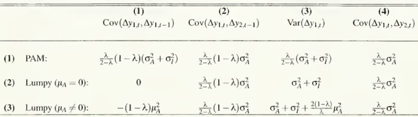
columns

2 and 4 in Table 4

we

observe that the cross-covariance terms under

PAM

and

lumpy

adjustment are thesame.8 Sincetheseterms will dominatefor sufficiently large

N

—

thereare

N(N

—

1) of

them,

compared

to

N

additional terms

—

itfollowsthatthebias vanishesas

N

goestoinfinity.

8

Thisissomewhatremarkable,since theunderlyingprocessesare quitedifferent. Forexample,consider thefirst-order

cross-covariance term. In thecase ofPAM,adjustmentsat alllags contributetothecross-covariance term:

Cov(Ay,,,,Ay2,,_1)

=

Cov(X

£(1

-X)

k

A/U

-k.

*X0

-^'^-l-/)

*>o ;>o

=

_X

X2(l-X)

w+,

Cov(AyI i,_Jt ,Aj5 il_1_l)

5>

:

u-*)

2/+ I

Bycontrast, inthe case of thelumpyadjustmentmodel,thenon-zerotermsobtainedwhencalculating thecovanance betweenAyj.,

and Ayij-1 areduetoaggregateshocksincluded both intheadjustmentofunit1 (in;)andunit2(inI

—

1). Idiosyncraticshocks

Table4:

Constructing

the

First

Order

Correlation

(1) (2) (3) (4)

Cov(Ayi

ir,Ayiif_i)

Cov(Ay

u

,Ay2.t-i) Var(Ay,,,)

Cov(Ay

M

,Ay2i,)

(1)

PAM:

^(l-XKoJ

+

of)

&(i-*)<>3

nK+°;)

_2-X°A

(2)

Lumpy

(fiA

=

0):

&(l-*)°5

_°5

+

G/

_2-X°A

(3)

Lumpy

((iA7^0):

-(1-X>2

&0-*K

°iW

+

^

_tf

_2-X°A

However,

the underlying bias

may

remain significant for relatively large valuesof

A

7

.

From

Table

4

it

follows that thebias forthe estimated first-orderautocorrelation originates

from

the autocovariance terms included in both the numerator and denominator.

The

first-order autocovariance term in the numerator

is zero for the

lumpy

adjustment model, while it is positive under

PAM

(this is the bias

we

discussed in

Section 2).

And

even though the

number

of terms with thisbiasisonly

N,

compared

with

N(N

—

1)

cross-covanance

terms with

no

bias, themissing termsare proportional to

G

_A

+

rj2, while those thatareincluded

areproportionalto

g

_a2,

which

isconsiderably smallerinall applications. This suggeststhat thebias remains

significant for relatively large values of

N

(more on this below)

and

that this bias rises with the relative

importanceof idiosyncratic shocks.

There

is asecond source ofbiasonce

N

>

1,relatedtothe varianceterm Var(Ayi,) in the

denominator

ofthefirst-ordercorrelation in (21).

While

under

PAM

thisvariance is increasing in A,varying

between

(when

A

—

0)and

G

_A

+

a

2

(when

A

=

1),

when

adjustmentis

lumpy

thisvarianceattainsthelargestpossible

valueunder

PAM, G

_A

+

o~2,independent oftheunderlyingadjustment speedA.Thissuggests thatthebiasis

more

important

when

adjustmentisfairly infrequent.9

Substitutingthetermsinthenumerator and denominatorof (21)

by

theexpressions inthe second

row

of

areirrelevant as farasthecovarianceisconcerned.Itfollowsthat:

Cov[Ayi,,,Ay2 ,,-i|E,i,,

=

1,£2,1-1

=

UuA^i]

=

min(lh,-l,/ 2,,-i)a^,

and averagingover/], and_/2,1-Lboth ofwhichfollow (independent) Poissonprocesses,

we

obtain:

Cov(Ayi,„Ay2,,_1

)=

^(l-X)^,

(22)

whichistheexpressionobtainedunderPAM.

9_To

furtherunderstandwhyVar(A>'i,)canbesomuch largerinaCalvomodelthan withpartialadjustment,wecomparethe

contributionto thisvariance ofshocksthattookplacek periods ago, V^,.

For

PAM

wehave

Var(Ay„)

=

Var(

£

X(l-X)*AyJ

f_k)

=

X

2

£

(1-X)

a

Var(AyJ,_,), (23)

k>0 k>0

Table4, anddividing numerator and denominator by

N(N

-

1)X/(2

—

X) leads to:

1-X

Pl

=

n

-

?

_3fv

(24)

This expressionconfirms our discussion. It illustrates clearly that the bias is increasing in

G//ga and

de-creasing inA.andN.

Finally,

we

note that a value of/x^ 7^ biases the estimates of the speed of adjustment even further.

The

reason for thisis that itintroduces a sort of"spurious" negative correlation in thetime series ofAyi,.

Whenever

the unitdoesnotadjust, itschangeis,inabsolutevalue,

below

the

mean

change.

When

adjustment

finally takesplace,pent-up adjustments are

undone

andtheabsolute change, on average,exceeds _\ha\.

The

product ofthese

two

termsis clearly negative,inducingnegative serialcorrelation.10

Summing

up, the biasobtained

when

estimating

X

with standard partial adjustment regressions can be expected to besignificant

when

eitherct^/g/,

N

or

X

is small, or |it.i| is large. Figure 2 illustrates

how

X

N

converges to X.

The

baseline parameters (solid line)are 11,4

=

0, A.

=

0.20.

Ga

=

0.03and G/

=

0.24.

The

solid line depicts the percentage bias as

N

grows. For

N

=

1,000, the bias is above

100%; by

the time

N =

10.000, it is slightly

above 20%.

The

dash-dot line increases

Oa

to 0.04. speeding

up

convergence.

By

contrast, thedash-dot line considersjxa

=

0.10,

which

slows

down

convergence. Finally,thedotted line

shows

thecase

where

X

doubles to0.40.

which

alsospeeds up convergence.

Corollary 2

(Slow Convergence)

The

biasintheestimatoroftheadjustment speedisincreasinginG/

and

I/I41

and

decreasingin

Oa

•

N

and

X. Furthermore, thefour parameters

mentioned

above determine the biasofthe estimator viaa decreasing

expressionofK.' '

Proof

Trivial. I sothat ^PAM

_=X

2 (1

_

x) 2* (02

+o

2)

Bycontrast, inthecase oflumpyadjustmentwehave

viunw

=

Fr{/i,,=Jk}VSff(Ay,il|/,_/

=t)

Pr{/,., =A-}[AVar(Ay,,|/„

=

1,1;,.,

=

1)

+

(I-X-)Var(Ay,,,|f,,r

=

0,&=0)]

=

\(\-\)

k-l

[lk{<?_A+<$)}.

VktismuchlargerunderthelumpyadjustmentmodelthanunderPAM.Withinfrequentadjustmenttherelevantconditional

distri-bution isamixture ofamassatzero (correspondingtonoadjustmentatall)andanormaldistribution withavariancethatgrows

linearlywithk(correspondingtoadjustmentint ). UnderPAM.bycontrast, V;, isgeneratedfromaanormaldistributionwithzero

meanandvariancethatdecreaseswithk.

We

alsohavethat/i,*

^

further increasesthebiasduetothe varianceterm,see entry(3,3) inTable4.

"Theresultsfora/ andkmaynot holdif\nA\ islarge. Fortheresults toholdweneed

N

>

1

+

(2-X)ti_A2/\a2_A.

When

_Ma

=

u

thisisequivalentto A'

>

1andthereforeisnot binding.

Figure2:

BiasasafunctionofNforvariousparameterconfigurations

to en 180 160 140 120 S" 100 a °- ₈₀ 1000 2000 3000 4000 5000 6000 7000 8000 9000 10000 Numberofunits:N 3.2

Applications

Figure 2

shows

thatthebias in theestimate ofthe speed of adjustmentis likely toremain significant, even

when

estimatedwithveryaggregateddata. In thissection

we

provideconcreteexamples based onestimates

forU.S.

employment,

investment,andpricedynamics.

These

series areinterestingbecausethereisextensive

evidenceoftheirinfrequentadjustmentat themicroeconorruc level.

Letusstartwith U.S. manufacturing

employment.

We

use theparametersestimated

by

Caballero,Engel,

andHaiti

wanger(

1997) withquarterlyLongitudionalResearchDatafile

(LRD)

data. Table5

shows

thateven

when

N

—

1,000,

which

corresponds to

many

more

establishmentsthan in atypical two-digit sectorofthe

LRD.

thebias remains

above

40

percent. That is, estimated speeds ofadjustment atthe sectoral level are likelytobesignificantly fasterthanthe true speed of adjustment.

The good

news

in thiscaseis thatfor

N

=

10,000,

which

is aboutthesize ofthecontinuous

sample

in

the

LRD,

thebiasessentiallyvanishes.

The

results for prices, reported in Table 6, are based on the estimate ofX, _Ha

and

04.

from

Bils and

Klenow

(2002), while a/is consistentwiththatfound inCaballeroetal (1997).,2

The

table

shows

that the

Togofromthea;computedforemploymentinCaballeroetal.(1997)tothatofprices,wenotethatifthedemandfacedbya

monopolistic competitivefirmisisoelastic,itsproduction functionisCobb-Douglas, anditscapital fixed(whichisnearly correct

athighfrequency),then (uptoa constant):

P*a

=

(

w

i-flir)

+

-°-l)1'i

where p* andI* denote thelogarithms offrictionlessprice andemployment, w, anda,, are the logarithm of thenominalwage

andproductivity,anda^isthelaborshare. Itisstraightforwardto seethataslongasthe mainsourceofidiosyncratic varianceis

demand,whichweassume,a/.

~

(1

—

a/Jo-/,.

.

Table 5:

Slow Convergence: Employment

Average

X

Number

of agents(N) 100 1,000 10.000

Number

35 of

Time

200

Periods (T) 0.901 0.631 0.523 0.852 0.548 0.436 0.844 0.532 0.417 0.400

Reported: averageof

OLS

estimates of X,obtainedviasimulations. Numberof

simulationschosentoensurethatnumbersreportedhaveastandard deviationless

than 0.002. Case T

=

°°calculatedfromProposition3. Simulationparameters:

X:0.40,jxa

=

0.005.aA

=

0.03,o/

=

0.25.Quarterlydata,fromCaballeroetal.

(1997).

biasremains significantevenfor

N

=

10,000. In thiscase,the

main

reason forthe stubbornbias isthe high

valueof0/

/oa

Table6:

SLOW

CONVERGENCE:

PRICES

Average

X

100

Number

ofagents(N) 1,000 10,000

Number

60

of

Time

500

Periods (7) 0.935 (if)14 0.908 0.542 0.902 0.533 0.351 0.279 0.269 0.220

Reported: average

OLS

estimatesofX, obtainedviasimulations. Numberof

simulationschosentoensurethatnumbersreportedhaveastandard deviationless

than 0.002. Case

T =

«*>calculatedfromProposition3. Simulation parameters:

X: 0.22 (monthlydata,Bilsand Klenow, 2002),nA

=

0.003,aA

=

0.0054, a,

=

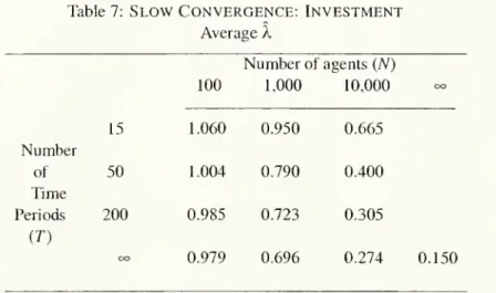
0.048.

Finally, Table 7 reports the estimatesfor

equipment

investment, the most sluggish of the three series.

The

estimate ofX,fi^ ar)d Oa<are

from

Caballero,Engel,

and

Haltiwanger(1995),and rj/ isconsistentwith

that found in Caballeroet al (1997).13

Here

the bias remainsvery large and significant throughout.

Even

when

N —

10,000,theestimatedspeedofadjustmentexceedstheactualspeedby

more

than

80

percent.

The

,3

To go fromthe07computedforemploymentinCaballeroet al(1997)to thatofcapital,wenotethatifthedemandfacedbya

monopolisticcompetitive firmisisoelasticanditsproductionfunctionisCobb-Douglas,then07,.

~

a/.. .

reasonsforthisisthecombination ofalowA.,ahigh\i_A (mostlyduetodepreciation),and a largerj/ (relative to

a

A).

Table 7:

SLOW

CONVERGENCE: INVESTMENT

Average

A.

Number

ofagents(N) 15 100 1,000 10,000 OO 1.060 0.950 0.665

Number

of 50 1.004 0.790 0.400

Time

Periods

200

0.985 0.723 0.305

CO

OO _{0.979 0.696 0.274 0.150}

Reported: averageof

OLS

estimatesof X, obtained via simulations. Number

ofsimulationschosentoensurethatnumbersreportedhaveastandard deviation

lessthan 0.002. Simulation parameters: X: 0.15 (annualdata,fromCaballeroet

al, 1995),nA

=

0.12,aA

=

0.056,07

=

0.50.

We

have

assumed

throughout that Ay* is i.i.d. Aside from

making

the results cleaner, it should be

apparent

from

thetime-to-build extensioninSection 2thataddingfurtherserial correlationdoes not

change

the essence of our results. In such a case, the cross correlations

between

contiguous adjustments are

no

longer zero, but the bias

we

have described remains. In any event, for each of the applications in this

subsection, there is evidence that the i.i.d. assumption is not farfetched (see, e.g., Caballero et al [1995, 1997], Bilsand

Klenow

[2002]).

4

Fragile Solutions:

Biased Regressions

and

ARMA

Correction

Can

we

fixthe

problem

whileremaining within the class oflineartime-series

models?

In this section,

we

show

that inprinciple thisispossible,butinpracticeitis unlikely (especiallyforsmallN).

4.1

Biased

Regressions

So

far

we

have

assumed

thatthe speedofadjustment is estimated using only information

on

the

economic

series ofinterest,y. Yetoften the econometrician can resort to aproxyforthe target y*. Instead of(2),the estimating equationis:

Ay,

-

( 1

-

X)Ay,-1

+

AAy,*

+

e,

,

(25)

with

some

proxyavailable forthe regressorAy*.

Equation (25) hints at a procedure for solving the problem. Since the regressors are orthogonal,

A

in principle can be estimated directly

from

the parameter estimate associated with Ay*, while dropping

the constraint that the

sum

of the coefficients

on

the right

hand

side add up to one.

Of

course, if the

econometriciandoes

impose

the latterconstraint, then theestimate ofA. will be

some

weighted average of

an unbiased and a biased coefficient, and hence willbe biased as well.

We

summarize

theseresults in the

followingproposition.

Proposition.4 (Bias with Regressors)

With the

same

notation

and

assumptionsasin Proposition3, considerthefollowingequation:

Ay?

=

fc Ayf_,

+&iAy,*+e„

(26)

where

Ay* denotes the average shock in periodt,

£Ay*

;/7V.

Then, if(26) is estimated via

OLS, and

K

definedin (19),

(i)without

any

restrictionsonbo

and

h\:

(ii) imposingbo

=

1

—b].

u

plinij^^b]

=

A

+

In particular,for

N

=

1

and

/1.4

=

0:

plimT_t

J

=

-^-(1-A),

(27) 1

+

K

plim_T

_{_J>}

x

=

A, (28)

X(l-X)

2{K

+

X)' i 1 !

~

_X

plim_T

^„b\

=

A

H

—

.

Proof

SeeCorollary

Bl

in theAppendix.

Of

course,inpracticethe"solution"aboveisnot veryuseful. First,theeconometrician

seldom

observes Ay* exactly, and(at least) thescaling parameters need tobe estimated. In thissituation, the coefficient

es-timate on the

contemporaneous

proxy for Ay* is

no

longer useful for estimating A, and the latter must be

estimated

from

theserialcorrelationoftheregression,bringingbackthe bias. Second,

when

the

econometri-cian does observe Ay*, theadding

up

constraint typically is linked to

homogeneity and

long-run conditions

,4

Theexpressionthatfollowsisaweighted averageof theunbiasedestimalorXandthebiased estimatorintheregression without

Av* asaregressor (Proposition 3).Theweight onthebiasedestimatorisXK/2(K

+

X),whichcorrespondstotheharmonicmean

ofXand K.

that aresearcher often will bereluctant todrop(seebelow).

Fast

Micro - Slow

Macro?:

A

Price-

Wage

Equation

Application

Inan intriguingarticle, Blanchard (1987) reachedtheconclusionthat the speed of adjustment ofprices to costchanges is

much

fasteratthedisaggregate thantheaggregate level.

More

specifically, he

found

that

prices adjustfaster to

wages

(and input prices) at the two-digit level than at theaggregate level. His study

considered seven manufacturing sectors and estimated equations analogous to (26), with sectoral prices in

theroleofy,and bothsector-specific

wages

and inputpricesasregressors(they*).

The

classic

homogeneity

conditionin thiscase,

which was imposed

in Blanchard'sstudy,isequivalentinoursetting tobo

+

b\

—

1 .

Blanchard's preferred explanation for hisfinding

was

based on the slowtransmission of price changes through the input-output chain. This is an appealing interpretation and likely toexplain

some

of the

dif-ference in speedofadjustmentat differentlevels ofaggregation.

However,

one

wonders

how

much

ofthe

findingcan be explained

by

biaseslikethosedescribedin this paper.

We

do

notattemptaformal

decompo-sitionbutsimply highlight thepotentialsizeofthebiasin price-wageequationsfor realisticparameters.

Matching

Blanchard's

framework

tooursetup,

we

know

that hisestimated sectoral

A

is approximately

0.18 whileatthe aggregatelevel itis0.135.15

Table 8:

Biased

Speed

of

Adjustment:

Price-Wage Equations

Average

A

Number

offirms(A7

)

100

500

1.000 5.000 10,000 oo

250

0.416 0.235 0.194 0.148 0.142 0.135

No.

of

Time

Periods, T:

oo 0.405 0.239 0.194 0.148 0.142 0.135

Reported: ForT

=

250, average estimateofXobtainedvia simulations. Numberof simulationschosentoensurethat

estimatesreportedhaveastandarddeviationlessthan 0.004. For

T

=

°°: calculatedfrom(28). Simulation parameters:

X:0.135andT

=

250(from Blanchard, 1987, monthlydata),nA

=

0.003,aA

=

0.0054 and07

=

0.048asinTable6.

Table 8 reportsthebias obtained

when

estimatingtheadjustmentspeed

from

sectoralprice-wage

equa-tions. It

assumes

that thetruespeed ofadjustment,A, is0.135,andconsiders various valuesforthe

number

offirmsin the sector.

The

table

shows

that forreasonable values of

N

there isasignificant

upward

bias in

theestimated value ofA,certainly

enough

toincludeBlanchard'sestimates.16

,5

_We

obtained theseestimatesby matching thecumulative impulse responsesreported inthe first two columnsofTable 8 in

Blanchard (1987) for 5, 6 and 7 lags. For the sectoral speeds we obtain, respectively, 0.167, 0.182 and0.189, while for the

aggregatespeedweobtain0.137.0.121 and0.146.The numbersinthemaintextaretheaverageX'sobtainedthisway.

16

Theestimated speedofadjustmentiscloseto0.18 for

N

=

1,000.

4.2

ARMA

Corrections

Let us

go

back tothecase ofunobservedAy*.

Can

we

fixthebias while remainingwithinthe class oflinear

ARMA

models? In the first part ofthis subsection,

we

show

that this is indeed possible. Essentially, the correction

amounts

toaddinganuisance

MA

termthat "absorbs"the bias.

However,

thesecondpartofthissubsectionwarnsthatthisnuisanceparameter needstobe ignored

when

estimating thespeed of adjustment. This is notencouraging, because in practice the researcher isunlikely

to

know when

heshouldorshouldnotdrop

some

ofthe

MA

termsbefore simulating (ordrawinginferences

from)theestimated

dynamic

model.

On

theconstructiveside,nonetheless,

we

show

that

when

N

issufficiently large,even if

we

do

notignore

thenuisance

MA

parameter,

we

obtain better

—

although stillbiased

—

estimates ofthespeed of adjustment

than withthe simplepartial adjustmentmodel.

4.2.1

Nuisance

Parameters

and

BiasCorrection

Let usstart withthepositiveresult.

Proposition 5 (Bias Correction) Letthe Technical

Assumptions

(see

page

10)hold}1

Then

Ayf

follows an

ARMA(l.l)

process with autoregressive

parameter

equal to 1

—

X. Thus, adding an

MA(1

) term to the

standardpartialadjustment equation(2):

Ayf

=

(l-X)Ayf

/

_1

+v,-ey,_

lj (29)

and

denoting by

X

N

any

consistentestimatorof one

minus

the AR-coefficientin theequationabove,

we

have

that:

plim_T-00/v

=

X.

The

moving

averagecoefficient, 9. isa "nuisance"

parameter

that

depends

on

N

(itconverges tozeroas

N

tendsto infinity), _fa.

Oa

an

d

°"/- VM?havethat:

Q=~{L-VL

2

_-4)>0,

with 2

+ X(2-X)(K-\)

L

\-X

and

K

definedin(19).

Proof

See

Theorem

Bl

intheAppendix. I

17

Strictly speaking, to avoid the case wherethe

AR

and

MA

coefficientscoincide, we need torule out the knife-edge case

N

-1

=

(2-\)n^/Xo^. Inparticular,when_ma

=

thisamountstoassuming

N

>

1

.

The

proposition

shows

thatadding an

MA(1)

termtothestandardpartialadjustment equationeliminates

the bias. Thisrather surprising result is valid forany level ofaggregation.

However,

in practicethis cor-rection is notrobust forsmall

N,

as the

MA

and

AR

coefficients are very similar in thiscase (coincidental reduction).18 Also, as with all

ARMA

estimation procedures, the time series needs tobe sufficiently long

(typically

T

>

100)toavoidasignificant small

sample

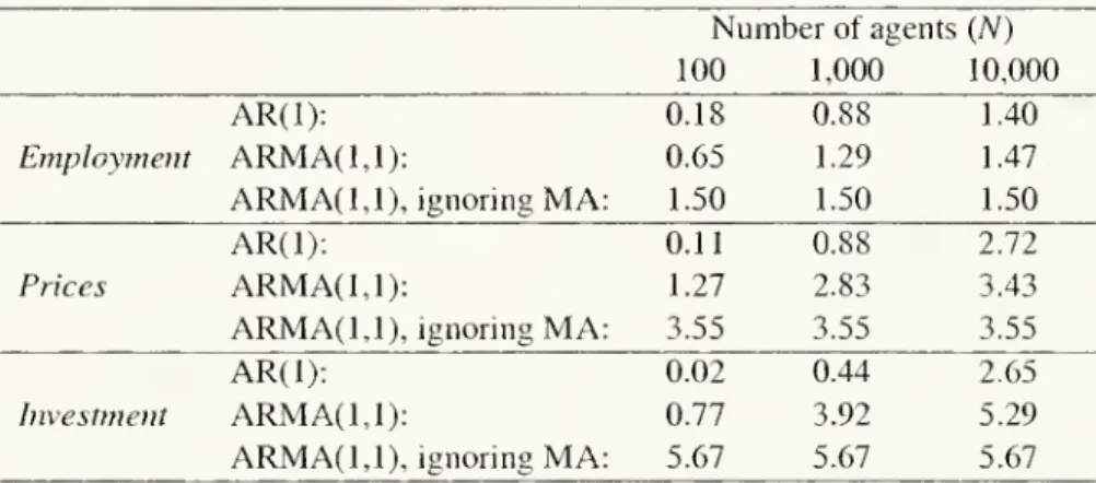
bias.

Table9:

ADJUSTMENT

SPEED

X:

WITH AND WITHOUT

MA

CORRECTION

Number

of agents(N) 100 1,000 10,000 AR(1): 0.18 0.88 1.40

Employment

ARMA(1,1):

0.65 1.29 1.47

ARMA(1,1),

ignoring

MA:

1.50 1.50 1.50

AR(1):

0.11 0.88 2.72

Prices

ARMA(1,1):

1.27 2.83 3.43

ARMA(1,1),

ignoring

MA:

3.55 3.55 3.55

AR(1):

0.02 0.44 2.65

Investment

ARMA(1,1):

0.77 3.92 5.29

ARMA(1,1),

ignoring

MA:

5.67 5.67 5.67

Reported: theoretical value ofT, ignoring small sample bias (7"

=

°°). "AR(1)" and

"ARMA(1,1)" refer to values ofx obtained from AR(1) and ARMA(1,1) representations.

"ARMA(l.l)ignoring

MA"

refersto estimate obtainedusing ARMA(l.l)representation,but

ignoring the

MA

term. Theresults inPropositions 3 and5wereusedtocalculate the

expres-sions forx.ParametervaluesarethosereportedinTables4,5and6.

Next

we

illustratethe extent to

which

our

ARMA

correction estimatesthecorrect response timein the

applications to

employment,

prices, and investment considered in Section 3.

We

begin

by

noting that the

expected response timeinferredwithoutdroppingthe

MA

termis:19

1-X

_{9_}

1-X

_{_}

Tma

~~~T^e

<-

X~~

x'

where

>

was

defined in Proposition 5, x denotes the correct expected response and x_ma the expected

responsethatisinferred

from

a non-parsimonious

ARMA

process(it couldbe an

MA(«),

an AR(°°)or, in

ourparticular case, an

ARMA(

1,1)).

The

third

row

in each ofthe applicationsin Table 9 illustrates the

main

result.

The

estimate ofx,

when

thenuisance termisusedinestimation but

dropped

forx-calculations, isunbiasedinallthe cases, regardless ofthevalueof

N

(notethatinordertoisolatethebiases thatconcern us

we

have

assumed

T

—

°°).

18

For example,ifji_A

=

0,wehavethatthe

AR

and

MA

termare identical for

N

=

I

.

19

SeePropositionAl intheAppendixfor aderivation.

The

first

and

second

rows

(in eachapplication)

show

thebiased estimates.

The

former repeatsourbasic

result while the latter illustratestheproblems generated by notdropping thenuisance

MA

term(Xma).

The

bias fromnot dropping the

MA

term is smallerthan that

from

inferringx from the first order

autocorrela-tion,20yetitremainssignificantevenat fairlyhighlevelsofaggregation(e.g.,

N

=

1,000).

5

Conclusion

The

practiceof approximating

dynamic

models withlinearones iswidespread and useful.

However,

itcan

leadto significantoverestimates ofthespeedofadjustmentof sluggishvariables.

The problem

is

most

severe

when

dealing with data at

low

levels ofaggregation or single-policy variables. For once,

macroeconomic

data

seem

tobebetterthan

microeconomic

data.

Yet this paper also

shows

that the disappearance ofthe bias with aggregation can be extremely slow.

For example, in thecaseofinvestment,thebiasremainsabove 80 percent even afteraggregatingacross all

continuousestablishments inthe

LRD

(N

=

10.000).

While

theresearcher

may

thinkthatattheaggregatelevel itdoesnotmatter

much

which microeconomic

adjustment-cost

model

generates the data, it does matter greatly for (linear) estimation of the speed of adjustment.

What

happened

to

Wold's

representation, according to

which

any stationary, purely non-deterministic,

process admits an (eventually infinite)

MA

representation?

Why,

as illustrated by the analysis at theend of Section 4,

do

we

obtain an

upward

biased speed of adjustment

when

using this representation for the

stochastic processat

hand? The problem

isthat Wold's representation expresses the variable ofinterest as a distributed lag (and therefore linear function) ofinnovations that are the one-step-ahead linear forecast errors.

When

the relation

between

the

macroeconomic

variableofinterest and shocksis non-linear,asisthe

case

when

adjustment islumpy. Wold's representation misidentifiestheunderlyingshock, leading tobiased estimatesof thespeed ofadjustment.

Put

somewhat

differently,

when

adjustment is lumpy, Wold's representation identifies the correct

ex-pectedresponse timetothe

wrong

shock. Also,

and

forthe

same

reason,the impulse response

more

gener-ally will bebiased.

So

will

many

of the

dynamic

systemsestimated in

VAR

stylemodels, andthe structural teststhatderive

from

such systems.

We

arecurrentlyworking on theseissues.

-°ThiscanbeprovedformallybasedontheexpressionsderivedinTheoremBI andPropositionAl intheappendix.

References

[1] Bils,

Mark

andPeterJ.

Klenow,

"Some

Evidence

on the Importance ofSticky Prices,"

NBER

WP

#

9069,July2002.

[2] Blanchard, OlivierJ., "Aggregate and Individual Price Adjustment,"Brookings Papers

on

Economic

Activity1,

1987,57-122.

[3] Box,

George

E.P., and

Gwilym M.

Jenkins,

Time

SeriesAnalysis: Forecasting

and

Control,

San

Fran-cisco:

Holden

Day, 1976.

[4] Caballero,RicardoJ.,

Eduardo

M.R.A.

Engel, and John C. Haltiwanger,"Plant-Level

Adjustment

and

Aggregate

Investment

Dynamics",

Brookings Papers

on

Economic

Activity,

1995

(2), 1-39.

[5] Caballero, Ricardo J.,

Eduardo

M.R.A.

Engel, and

John

C. Haltiwanger, "Aggregate

Employment

Dynamics:

Building

from

Microeconomic

Evidence",

American

Economic

Review,

87

(1),

March

1997, 115-137.

[6] Calvo, Guillermo, "StaggeredPrices inaUtility-Maximizing

Framework,"

Journal of

Monetary

Eco-nomics, 12, 1983, 383-398.

[7] Engel,

Eduardo

M.R.A.,

"A

Unified

Approach

to the Study of

Sums,

Products,

Time-Aggregation

and

otherFunctions of

ARM

A

Processes",JournalTime Series Analysis,5, 1984, 159-171.

[8] Goodfriend, Marvin, "Interest-rate

Smoothing

andPrice Level

Trend

Stationarity," Journal of

Mone-tary

Economics,

19, 19987,pp. 335-348.

[9] Majd,

Saman

and Robert S.Pindyck,

"Time

toBuild,OptionValue,and InvestmentDecisions," Jour-nalof Financial Economics, 18,

March

1987, 7-27.(1987).

[10]

Rotemberg,

JulioJ.,

"The

New

Keynesian Microfoundations," in O. Blanchard

and

S. Fischer (eds),

NBER

Macroeconomics

Annual, 1987,

69-104.

[11] Sack, Brian, "Uncertainty, Learning, and Gradual

Monetary

Policy," Federal Reserve

Board

Finance

and

Economics

DiscussionSeriesPaper34,

August

1998.

[12] Sargent,

Thomas

J., "Estimation of

Dynamic

Labor

Demand

SchedulesunderRational Expectations,"

Journal ofPolitical

Economy,

86, 1978.

1009-1044.

[13]

Woodford,

Michael, "Optimal

Monetary

PolicyInertia,"

NBER

WP

#

7261,July 1999.

d&y,+k [ de,

lk>okh

and x

=

—

-= i.

/md

V'(l) _{__}

S*>i*V*

Appendix

A

The

Expected

Response

Time

Index:

x

Lemma

Al

(tfor

an

Infinite

MA)

Consider a

second

orderstationary stochasticprocess

Ay,

=

_^Wk^t-k,

k>0

with \\Iq

=

1, _£*>()¥*

<

°°'

^

le £' '

5 uncorrelated,

and

e, itncorrelated with Ay,_i,Ay,_2.... Assw/Me ?/i«r

^M

—

Yk>o^VkZ hasallitsrootsoutside theunit disk.

Define:

Ik

=

I

Then:

Proof

ThatIk

=

ty* istrivial.

The

expressions forx then follow

from

differentiating *¥(z) andevaluatingat

z=l.

I

Proposition

Al

(xfor

an

ARMA

Process)

Assume

Ay,follows

an ARMA(p.q):

P 9

Ay,

-Yj

fa&yt-k

=

e,

-

X

Q

k£,-k-k=l k=\

where

$>{z)

=

1

—

_Y,k=\<J*JtS*a,!

^

®(z)

—

1 ~~_Sf=i6*z* 'iflve«// r/iefrroorroutsidethe unit disk. The

assump-tionsregarding theE,'sare the

same

as in

Lemma

A

1. Definexasin(30). Then:

Proof Given

theassumptions

we

have

made

about theroots of<J>(z) and 0(z),

we

may

write.

0(L)

Ay

<

=

*(Z)

E_"

where

L

denotes thelagoperator.

Applying

Lemma

Al

with0(z)/4>(z) intheroleof*F(z)

we

then have:

'

©(i)

*(i)

"

1-zjLi**

i-iLi

6

*'

Proposition

A2

(x for a

Lumpy

Adjustment

Process) ConsiderAy, inf/iesimple

lumpy

adjustment

model

(8)

and

x<te/inerf in (/4). 77ienx

=

(1

-

X)/X.21

2

'Moregenerally,ifthenumberof periodsbetweenconsecutive adjustmentsarei.i.d.withmeanm, thent

=

m—

1.Whatfollows

isthe particularcasewhereinterarrivaltimes follow aGeometricdistribution.

Proof dAy

t+k/dAy* isequaltoone

when

theunit adjustsattimet

+k,

nothavingadjusted

between

timest

and

t

+

k—1,

andisequaltozerootherwise. Thus:

/*

=

E,

dAy

l+k

dAy;

Prfe+*

=

1 , £,+*_,

= ^

+ ,_2

=

...

=

&=

0}

=

X(l

-

X) k . (31)

The

expressionforx

now

followseasily.

Proposition

A3

(xfor aProcess

With

Time-to-build

and

Lumpy

Adjustments)

Considertheprocess

Ay

t

withboth gradual

and lumpy

adjustments:

ith

K

K

Ay,

=

Yj

tyk&yt-k

+

(1

-

X

<WAy,,

A=l k=l ll-l k=0 (32) (33)

where

Ay* is i.i.d. with zero

mean

and

variance

O

2

.

Definex by:

Then:

Zjt>o^E, SAy;

Si>oE

dby, +k

3Ay,-Proof

Notethat:

E, 9Ay,_+k [ dAy;

3Ay

r+*9Ay,_+j

y

E

;

e

' [d&yt+j dAyf k

SB,

7=0

Gt_j

Ay, +J Ay,*

2,Gk-jH

Jt (34) ;=0

where, from Proposition

Al

and

(31)

we

have that the

G

k are such that G(z)

=

£*>o<j*z*

=

l/Q>(z), and

H

k

=

X{\

-

X) k

. Define

H(z)

=

E*>ofl*Z* and I{z)

=

G{z)H(z). Noting that the coefficient ofz* in the

infiniteseries I(z)is equalto7*in (34),

we

have:

r(i)

g'(i) //'(i)

_sf

₌₁

^

i-A

""

7(1)

"

G(l)

+

//(1)

_l-EJ^fe

A

B

Bias Results

B.l

Results

in

Section 2

Inthissubsection

we

proveProposition 2andCorollary 1. Proposition 1 isaparticularcase ofProposition3,

which

isprovedin Section B.2.

The

notation

and

assumptionsare the

same

asinProposition

A3.

Proof

ofProposition2

and

Corollary 1

The

equation

we

estimate is:

Ay,

=

Y,

ak

A

yt-k

+

v,. (35)

*=i

whilethe true relation isthatdescribed in(32)

and

(33).

An

argument

analogous to that given in Section 2.2

shows

that the second term on the right

hand

side

of(32), denoted byw, in

what

follows, is uncorrectedwith Ay,_£, k

>

1. Itfollows that estimating (35) is

equivalenttoestimating (32) with errorterm

*»

=

= (i-Efo&XAtf-*.

andtherefore:

f 4>;.

ifk=l,2,-,K,

plimr_„<5it

=

<

[ ifk

=

K+l.

The

expression for

pUm^^^t

now

follows

from

Proposition

A3.

|

B.2

Results

in

Sections

3

and

4

In thissection

we

prove Propositions3, 4,and 5.

The

notation and assumptions arethoseinProposition 3.

The

proofproceeds via a seriesof

lemmas.

Propositions 3 and5 areproved in

Theorem

Bl. while

Proposi-tion4isprovedin Corollary Bl.

Lemma

Bl

Assume

X]

and

Xjarei.i.d.geometric

random

variables with

parameter

X, sothat

Pr{X

=

k}

=

X(l

-X)

k

-\k=

1,2,3,... Then:

m)

=

I

Vkrpf,]

=

^.

Inparticular, theI,

-,'s (defined in the

main

text)are allgeometric

random

variables with

parameter

X.

Furthermore, /,.,

and

ljsareindependentifi

^

j.

Nextdefine,for anyintegerslargeror equal thanzero:

Ml

=(°.

_fy

[

min(Xi

—s

ifX

x

<

s,

-s,X

2)

ifX

x

>s.