The seasonal cycle of atmospheric CO 2 : A study based on the NCAR Community Climate Model (CCM2)

HAL Id: hal-02923800

https://hal.archives-ouvertes.fr/hal-02923800

Submitted on 28 Oct 2020

HAL is a multi-disciplinary open access

archive for the deposit and dissemination of

sci-entific research documents, whether they are

pub-lished or not. The documents may come from

teaching and research institutions in France or

abroad, or from public or private research centers.

L’archive ouverte pluridisciplinaire HAL, est

destinée au dépôt et à la diffusion de documents

scientifiques de niveau recherche, publiés ou non,

émanant des établissements d’enseignement et de

recherche français ou étrangers, des laboratoires

publics ou privés.

The seasonal cycle of atmospheric CO 2 : A study based

on the NCAR Community Climate Model (CCM2)

D. J. Erickson Iii, P. Rasch, P. Tans, P. Friedlingstein, P. Ciais, E.

Maier-Reimer, K. Six, C. Fischer, S. Walters

To cite this version:

D. J. Erickson Iii, P. Rasch, P. Tans, P. Friedlingstein, P. Ciais, et al.. The seasonal cycle of

at-mospheric CO 2 : A study based on the NCAR Community Climate Model (CCM2). Journal of

Geophysical Research: Atmospheres, American Geophysical Union, 1996, 101 (D10), pp.15079-15097.

�10.1029/95JD03680�. �hal-02923800�

JOURNAL OF GEOPHYSICAL RESEARCH, VOL. 101, NO. D10, PAGES 15,079-15,097, JUNE 27, 1996

The seasonal

cycle of atmospheric COz: A study based

on the NCAR Community Climate Model (CCM2)

D. J. Erickson III,• P. J. Rasch,

2 p. p. Tans, 3 p. Friedlingstein,•,4

P. Ciais, 5

E. Maier-Reimer? K. Six,6 C. A. Fischer,• and S. Walters,•

Abstract. A global three-dimensional atmospheric model, the NCAR CCM2 general circulation model, has been adapted to study the hourly to yearly variability of CO2 in the atmosphere. Features of this CCM2-based model include high spatial resolution (2.8 ø x 2.8 ø latitude/ longitude), 18 vertical levels, a 15-min time step, and an explicit, nonlocal atmospheric boundary layer parameterization. The surface source/sink relationships used include exchange with the ocean, the terrestrial biosphere, biomass burning, and fossil fuel release of CO2. The timing and magnitude of the model seasonal cycle are compared to observational data for 28 sites. The seasonal cycle of atmospheric CO2 is generally well predicted by the model for most of the northern hemisphere, but estimates of the amplitude of the seasonal cycle in the southem hemisphere are overpredicted. To address this aspect more rigorously, we have used the

monthly surface oceanpCO2 maps created by the Max-Planck-Hamburg ocean general circulation model to asses the ocean seasonality on the atmospheric surface CO2 seasonality. The globally averaged interhemisphehc gradient in atmospheric CO2 concentrations, as cornputc•d with the chosen source/sink distributions, is a factor of two too high compared to data, and selected longitudinal bands may be up to 50% higher than the zonal mean. The high temporal resolution of this model allows the infrequent yet real extrema in atmospheric CO2 concentra- tions to be captured. The vertical attenuation of the seasonal cycle of atmospheric CO2 is well simulated by the boundary layer/free troposphere interaction in the model in the northern hemisphere. Conversely, an increasing amplitude of the seasonal cycle aloft is found in the midlatitude southern hemisphere indicating interhemispheric transport effects from north to south. We use two different models of the terrestrial biosphere to examine the influence on the computed seasonal cycle and find appreciable differences, especially in continental sites. A global three-dimensional chemical transport model is used to assess the production of CO2 from the oxidation of CO throughout the volume of the atmosphere. We discuss these CO + OH --> CO2 + H results within the context of inverse model approaches to ascertaining the global and regional source/sink patterns of CO2. Deficiencies in the model output as compared to observational data are discussed within the context of guiding future research.

1. Introduction

It is clear from experimental evidence that the atmospheric

concentration of CO2 has increased from-280 ppm to -350

ppm since the industrial revolution started about 1800 [Keeling et al., 1976; Raynaud et al., 1993]. One of the many aspects of the carbon cycle that is at present not sufficiently quantified is how and where the roughly 50% of the total anthropogenic CO2 released to the atmosphere has been absorbed by sinks on the Earth surface. There have been

arguments put forth for oceanic uptake as well as increased

carbon storage in the terrestrial biosphere [Bolin, 1960;

Broecker et al., 1979; Tans et al., 1990; Quay et al., 1992;

Melillo et al., 1993]. One of the most important constraints on the various global three-dimensional numerical simulations of the atmospheric CO2 cycle is the inter-hemispheric gradient [Denning, 1994]. Since most 2-D and three-dimensional

Copyright 1996 by the American Geophysical Union.

Paper number 95JD03680.

0148-0227/96/95JD-03680509.00

atmospheric models tend to overpredict the interhemispheric

gradient, it has been suggested that there may be a "missing"

sink in the northern hemisphere surface boundary flux

conditions.

Here, we describe a global three-dimensional atmospheric

CO2 model based on the semi-Lagrangian transport (SLT)

code in the NCAR (National Center for Atmospheric Research) community climate model, version 2 (CCM2). The main emphasis of this paper will be to introduce the salient aspects of the SLT/CCM2 transport model and compare the model predictions with atmospheric CO2 observations [e.g. Fung et al., 1983, Denning et al., 1995]. We compare the phasing and

amplitude of the model seasonal cycle of atmospheric CO 2

with the National Oceanic and Atmospheric Administration/

Climate Monitoring and Diagnostics Laboratory

(NOAA/CMDL) observations at 28 sites distributed globally [Conway et al., 1988; Thoning et al., 1989] and aircraft measurements over Cape Grim, Tasmania [Pearman and Beardsmore, 1984] and Sendai, Japan [Tanaka et al., 1987].

We examine two treatments each of the ocean and terrestrial

biosphere exchange of CO2 with the atmosphere.

15,080 ERICKSON ET AL.: SEASONAL CYCLE OF ATMOSPHERIC CO2

2. Model Description

The transport of moisture and tracers is done in CCM2 by

using a three-dimensional "shape-preserving" semi-

Lagrangian transport formalism [Rasch and Williamson,

1990a; Williamson and Rasch, 1989]. The transport scheme

was originally developed for the transport of water vapor in a

general

circulation

model

[Rasch

and Williamson

1990b;

1991]. More recently, it has been succesfully used for the simulation of stratospheric aerosol transport [Boville et al.,

1992], for the transport

of t4

C and the transport

of CFCs in

troposphere [Hartley et al. 1994]. We performed detailed tests

of the mass conservation of CO 2 and found that mass was

conserved to within 1% over 5 years. The F-11 tracer

experiments compare reasonably well with the Atmospheric

Lifetime Experiment/Global Atmospheric Gases Experiment

(ALE/GAGE) observational data with respect to seasonal

cycle amplitudes, variability, and year-to-year atmospheric accumulation [Hartley et al., 1994]. The shape-preserving transport algorithm can maintain very sharp gradients without introducing overshoorts or undershoots and diffuses only at the smallest scales of the model.

The planetary boundary layer (PBL) parameterization of

Holtslag and Boville [1993] is a nonlocal scheme based on

the work of Troen and Mahrt [1986], and Holtslag et al.

[1990]. The parameterization diagnoses the boundary layer

height and uses a prescribed profile of diffusivities below this

level. The parameterization includes the typical down

gradient diffusion as well as a less typical nonlocal transport term within the convective boundary layer (sometimes called a countergradient transport term). Above the PBL a local

vertical diffusion scheme is used. A parameterization of

momentum flux divergence produced by stationary gravity

waves arising from flow over orography is included, following

McFarlane [1987]. A simple mass flux scheme developed by

Hack (1993) is used to represent all types oœ moist convection.

The cloud fraction and cloud albedo parameteriza0ons are a

generalization

of those

of Slingo [1987]. The solar

?adiative

heating is computed using a delta-Eddington parameterization

with 18 spectral bands [Briegleb, 1992]. Sea surface

temperatures are specified by linear interpolation between the climatological monthly mean values of Shea et al. [1990].

Surface fluxes are calculated with stability dependent transfer coefficients between the surface and the first model level,

detailed by Holtslag and Boville [1993]. Both diurnal and annual cycles are included. Radiative heating rates are

calculated periodically and held constant between

calculations. Absorptivities and emissivities are calculated every 24 hours. Radiative heating rates are calculated every 1.5 hours. The land temperature is calculated by a four-layer

diffusion model with soil heat capacities specified for each

layer to capture the major observed climatological cycles. The land has specified soil hydrologic properties [Hack et al.,

1994].

3. Surface Boundary Fluxes

The uptake and release of atmospheric CO 2 with various surface boundary carbon reservoirs imparts a strong signal on

observed atmospheric CO2 concentrations on time scales

ranging from days to years. In our calculations we have selected the four main boundary flux conditions that are presently thought to be important for simulating the

variability of atmospheric CO 2 on daily to yearly timescales.

The terrestrial biosphere is one of the most important

components of the Earth system that influences atmospheric

CO2 concentrations on daily to seasonal timescales. The

ocean is thought to be important in the global CO2 budget on

seasonal to yearly timescales. Land use change, especially

biomass burning in developing countries, may contribute

significantly to the observed increase in atmospheric CO2

concentrations and we use a source term that has a weak seasonality. Fossil fuel combustion is the main single

anthropogenic source of atmospheric CO2 and we use a source that is without a seasonal cycle. The deforestation and

terrestrial biosphere fluxes are constructed from monthly means

that are interpolated to give daily values. Figure 1 shows the globally integrated net fluxes from each of our initial four source/sink parameterizations: fossil fuel and deforestation are both positive over the seasonal cycle; the ocean is a net sink

over

the seasonal

cycle

and the terrestrial

biosphere

imparts

the majority of the variability of the seasonal cycle and sums

to roughly zero over the seasonal cycle. Table 1 shows the

annual integrated net sources. Note that the sum of the global

fluxes does not add up to the atmospheric CO2 increase that

has been observed over the last decade, namely, 3.0 Gt (10 t2

kg) C yr 1, as observed from the NOAA global flask sampling network. The main emphasis of this work, however, is the

seasonal cycle of atmospheric CO2 and we are not concerned

here with decadel time scale changes in the mean atmospheric

CO2 concentration. We use the four surface boundary CO2

NET SURFACE FLUX FOR BOUNDARY DATASETS ... x ... t ... .t• ... i t ...

,,,..

-2 -

\\

II

-

- --

fos

\\

-

- ---

',

-

sum

, t

_

Figure ]. The net surface fluxes used in the initial version of

the model. The fossil fuel tracer is always positive and is assumed to be invariant over the seasonal cycle. The land use change (deforestation) tracer is also always positive and has a slight seasonality. The ocean is a net sink for atmospheric

CO•_ and •s also assumed to be co•stam over the seasonal

c•cle. Note that the largest temporal forcin; o• the

atmosphe•c CO• bud;et •s •m the te•es•al b•osphere.

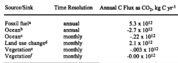
ERICKSON ET AL.: SEASONAL CYCLE OF ATMOSPHERIC CO2 15,081 Table 1. Annual Magnitude of the Global Source/Sink Terms

Used in Model Runs

Source/Sink Time Resolution Annual C Flux as CO2, kg C yr -1

Fossil fuel a annual 5.3 x 1012

Ocean b annual -2.7 X 1012

Ocean c monthly -.22 x 1012

Land use change d monthly 2.1 x 1012

Vegetation e monthly -.003 x 1012

Vegetation f monthly -0.00 x 1012

aMarland and Rotty [1984].

bBroecker et al. [1986] pCO 2 field with a 14C consistent transfer velocity.

CMax-Planck-Institute far Meteorlogie-Hamburg (MPI-H) three-

dimensional ocean model.

dlncluding Biomass Burning, blueller [ 1992].

eFung et al. [ 1987].

fFriedlingstein et al. [1992].

flux estimates summarized in Figure 1 in our initial model runs and compare and contrast the results from these runs with

additional model runs employing the Friedlingstein et al.

[1992] terrestrial biosphere model and the Max-Planck Institute (MPI-Hamburg) ocean model.

ocean temperature, salinity, total inorganic carbon, and alkalinity [Weiss, 1974]. It is straightforward to see that the

sense of the air-sea flux is determined by the deviations of

pCO2so

from pCO2*. When the surface

ocean is

undersaturated with respect to the atmosphere, the flux of CO2

is into the ocean; when the ocean is supersaturated with respect to the atmosphere, the converse is true. It is important to note that there is substantial uncertainty in the global

distribution of both pCO2so and K w [Etcheto and Merlivat, 1988; Erickson, 1993]. The global mean transfer velocity has been made consistent with the observed oceanic uptake of 14C

produced by nuclear testing.

The partial pressure of CO2 in surface ocean waters (pCO2)

is a complicated function of several different physical, chemical, and biological processes. It is important to note that several recent experimental studies have observed much variability in the surface ocean CO2 content [Watson et al.,

1991; Wong and Chan, 1991]. While it is currently believed that the main source term that influences the seasonal cycle of atmospheric CO2 is the terrestrial biosphere, in the southern hemisphere there may be an important seasonal forcing due to the ocean. This will be the topic addressed when we compare and contrast the atmospheric CO 2 results obtained from using

two different ocean treatments.

3.1. Terrestrial Biosphere

The atmosphere exchanges carbon with the terrestrial

biosphere on a variety of time scales, one of the most

prominent being the seasonal cycle. In the phase 1

calculations we have used the monthly global grids described

by Fung et al. [1987]. These global source/sink terms sum to roughly zero for the annual cycle. In addition, note that each element of the terrestrial source/sink grid sums to approximately zero over the annual cycle, Table 1. The overall seasonal cycle of all source/sink terms is clearly dominated by

variation in atmosphere-terrestrial biosphere CO2 exchange.

In a section below we compare the model runs of the Fung et al. [1987] sources with those ofFriedlingstein et al. [1992] with particular emphasis on the amplitude and phasing of the seasonal cycle at middle-high latitudes of the northern

hemisphere.

3.2. Ocean

The ocean has long been known to influence the

atmospheric concentrations of many trace gas species. The

distribution of the partial pressure of CO2 (pCO2) in the

global surface ocean is one of the important factors in modeling air-sea CO2 transfer (Sarmiento and Sundquist,

1992). In these calculations we have used the annual mean

pCO2 grid of Broecker et al. [1986] and a monthly model estimate of pCO2 produced by the Max-Planck-Institut far

Meteorologie, Hamburg, ocean GCM. The pCO2 grid has been

converted to a flux map via the application of a 14CO2 consistent transfer velocity, as described in Equation (1)

F = K w [pCO2*- pCO2so] (1)

where F is the net flux and may have units of umol cm -2 h-•

when

Kw

is the

transfer

velocity

(cm

h-l),

p CO2'

is the partial

pressure of CO 2 in surface sea water in equilibrium with an

atmospheric CO2 wet mixing ratio of 350 ppm (gmolecules

cm-3) and pCO2s o is the measured or modeled CO2 partial

pressure in surface ocean seawater (umol cm-3). Note that

pCO2* is a nonlinear

solubility-related

function

of surface

3.3. Land Use Change/Biomass Burning

The release of carbon to the atmosphere from land use

changes, mostly conversion of tropical forest to cropland or

pasture (including biomass burning), has been accounted for

by using the global distribution of these processes as

described by Mueller [1992]. The total annual flux is

estimated as 2.1 Gt C per year. Note that in the time series of

the four different sources over the annual cycle (Figure 1) there

is a slight seasonality in the land use change emissions,

largely related to the amount of precipitation over the tropical forest regions. Clearly, most biomass burning is occurring in

tropical regions of developing countries such as Brazil

[Woodwell et al., 1983]. The small negative values represent

those areas that have been altered by mankind and are

presently regrowing as cultivated crops or new forest growth.

3.4. Fossil Fuel

The flux of CO2 to the atmosphere associated with the

combustion of fossil fuel is an important component of the contemporary cycle of atmospheric CO 2 [Keeling, et al., 1976;

Marland and' Rotty, 1984]. Based on experimental and

modeling evidence, the observed increase in atmospheric CO2 is primarily due to the addition of-5 Gt C (as CO2) yr-• being added by the fossil fuel source [Revelle and Suess, 1957]. Here, we use a source function that is invariant in time over the annual cycle. The annual flux that we have used in this

work is 5.3 Gt C (as CO2) yr-1 [Rotty, 1987a, b]. The source term is known to be somewhat seasonal in character [Marland and Rotty, 1984]; however, this variability is thought to be of

the order of 10-20% and we do not include the monthly

variability in these first numerical experiments with the model.

4. Model Diagnostics

The model has been run for 6 years with the output data

archived every 12 hours. We have selected years 5 and 6 as

15,082 ERICKSON ET AL.' SEASONAL CYCLE OF ATMOSPHERIC CO2 ALT / \ Flask. _ r, ½u i / -5 -10 v ' ASC : I t : I t

• 1 •

/•

Model

I t

l.,k=

1-,-,

-

AMS digital filter with a frequency cutoff for detrending of 0.5

/^•

•

cycles

yr

-1

fbr

both

the

data

and

the

model

output.

The

\\

ii

.

/?%.

i

Flask/r,

!• treated

data

sets

to get

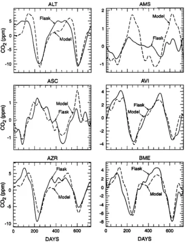
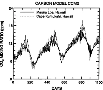
Figure

2. The general

characteristics

of

both data and observations are larger (>5 ppm CO2) seasonal amplitudes of CO2 in the northern hemisphere and smaller (<5

ppm CO2) in the southern hemisphere.

Table 2 shows the amplitude of the modeled and observed AVI seasonal cycle for each of the 28 stations plotted as function of

-'''

•'''

•'''

•' '- latitude

and

summarized

in Figure

3. The seasonal

cycle

i//A •

amplitudes

in

the

northern

hemisphere

are

much

larger

than

in

•'

tMødelx'//

•

-

(45øN,

124øW),

shows

the

influence

of sector

sampling

on the

/

/

subsequently

derived

seasonal

cycle. The observations

are

=

• t

• /= restricted

at this

station

to conditions

when

the

winds

are

_ \

i •V •x• fromoffthe

Pacific

so

asto

sample

amarine

,background

,

-• • • I • • • f • • • I • •= condition. This explains why the summer 'drawdown' of

BME atmospheric CO2 due to the increased activity of the terrestrial

.... •''' •''' •' ': biosphere as computed by the model does not appear so

=-

/.//•1\

•

Flask'x••

strongly

in the observational

record. This is a common

feature

• //.•/' •

/,

of several

of the

experimental

sites. In southern

hemisphere

•x•; XModell

/; regions

the

model-computed

seasonal

cycles

are

overestimated

•/

V the

seasonally

varying

surface

ocean

pCO2

field

of

the

MPI-H

_ ocean general circulation model to drive the atmosphmic

_

:, , • I • • • I , • • I • •= model. In section 4.1 we will discusss in detail the seasonal

0 200 400 600 cycles at selected geographically representative stations.

DAYS DAYS

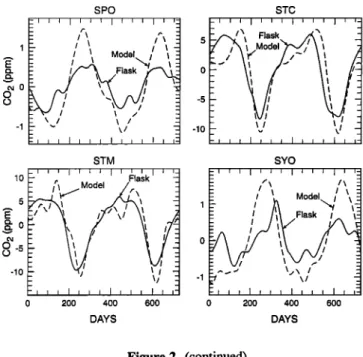
Figure 2. The CCM2-based carbon cycle model predicted

atmospheric CO 2 concentrations compared with the National

Oceanic and Atmospheric Administration/Climate Monitoring

and Diagnostics Laboratory (NOAA/CMDL) observational data for 28 sites around the world. See Table 2 for location

information. Day 1 corresponds to January 1.

comparison with observational data. The seasonal cycles in

atmospheric CO2 mixing ratios at a variety of observational

stations are compared with the model predictions. The

o 0-5 -10 BMW

_-'

,/• Flask.x• 10

/•'

\\•

;•Model\t

/ 5

i

IV

V '10

• /1, Flask /\,

--=_

computed

interhemispheric

gradient

inatmosphcric

CO?.

and

b''' •'''

•'''

•' 'd I•''' i,,,

•,,, •, '•1

the

of altitude

phasing

and

are

amplitude

also

discussed

of

the

within

seasonal

the context

cycle

as

a

function

of the

•o

• /•Flask_

I= t\ .Model

•./

"It I 1

•- .?'\, .Flask

observations.

• i••

•,•.//'•

• • o

4.1. Seasonal Cycle Simulations -•o -3

We

have

selected

28 stations

with

which

to objectively

compare

the

model.

The

CMDL

data

used

for comparison

with

½HR

½MO

the

model

output

for

years

5-6

are

from

1989

and

1990.

Th• =_--

/• xFlask

• 10

observational

data

years

selected

for

comparison

to the

model 2___ Model

I •

• 0

were

chosen

to be

relatively

free

of obvious

climate

c•li/'L•5 ) l/"x

"anomalies"

such

as

E1Nino

orPinatubo

anddisplay

amore

!i,j'

••

//xf•x

I .10

or less

"climatological"

character

that is appropriate

for o• 0

•

•

examination

of

seasonal

cycles.

In

some

cases

the

years

used

-1

= •/

•X• -20

were

different

from

1989

and

1990

due

to the

incompleteness

---,,

i I,, r I r r, I, ,a -30

of the observational

data during

this period. In those cases,

0

200 400 •00

0

200 400 •00

model-data comparison. Figure 2 shows the model-data

ERICKSON ET AL.: SEASONAL CYCLE OF ATMOSPHERIC CO 2 15,083 GMI • 0 0-2 /

ø

d

¾

4 kr•'\ ' Flask

x.

VJ//%\

\ _-

• 4 • j • flask

0 20o 4oo 60o

DAYS lO 5 o -5 -lO KEY [ I i , I I ] I- _ ask"--,.¾,X^ \

the residuals for the NOAA/CMDL observations. The vast

majority of the residuals are within 1 ppm in the model run as well as in the data, which is encouraging. In addition, there

appears to be a clear seasonality in the model residuals that

appears to some extent in the data. This seasonality has enhanced variability in the late winter-spring seasons that maybe related to transport issues [Harris and Kahl, 1990; Harris et al., 1992]. This 12-hour timescale variability

-,• I• • • I,• • I• r indicates the possibility of up to 3-4 ppm variability in MB½ atmospheric CO2 concentrations that are related to the local

r\/Model

-- synoptic

scale

meteorology.

Indeed,

a power

spectrum

of the

/•i '/ •\

_{} \'• ],,,-'}

_\i

model

_significant

output

_power

as

_in

well

_the

_{3 to}

as

_4-day

the

observational

_band.

data

show

4.1.2. Bermuda. Bermuda (33øN, 89øW) is generally

downwind from the North American continent, which has strong terrestrial biosphere and fossil fuel emission signals.

The seasonal cycle of the model and data are presented in

Figure 6. The detrended model predictions are in reasonable

MLO

--- Flask----*/'• --

L//•\/..-Model

///,

1 _--

0 200 400 600

DAYS

agreement with the observations with the amplitude of the seasonal cycle averaging about 8.7 ppm. The observational data show a somewhat anomalous spring-summer minimum in

1991 that does not appear in the model. This could be related

to interannual variability in the source/sink terms in the real world that are not included in the present model formulation. Note that the fall 'bump' in the observational data is also replicated by the model and is related to a seasonal release of carbon from the terrestrial biosphere as well as an enhanced

transport of fossil fuel CO2 during this time period. This

Figure 2. (continued)

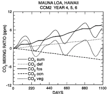
4.1.1. Mauna

Loa. Figure

4 shows

the model-observation e

compari,;on, smoothed and detrended, for three annual cycles at Mauna Loa (19.5øN, 155.6øW). Here, to facilitate the

interpretation

of climatological

seasonal

cycle,

we smooth

by

• 0

averaging

every

7 days

and

then

fit a cubic

spline

to the c•.2

resulting

points. This removes

much

of the shorter

timescale

variability

present

in Figure 2. The seasonal

cycle is

observations, with several stations being offset by a few weeks to a month. Note that in Figure 2, using the Fast

Fourier Transform approach to get the amplitude of the

seasonal cycle, the computed amplitudes are somewhat higher than in this analysis. The relative difference between the model and the observations is still roughly 1 ppm CO2. This points out that great care must be taken in using a variety of statistical methods to analyze both model output and data,

especially when comparing results between diverse research

groups.

An important

test

of model

variability

is the ability of the c•

model

to replicate

the deviations

of individual

events

from o-s

some long-term mean. The model is run at a 15-min time step -10

and we choose to save a three-dimensional model 'realization' every 12 hours. Figure 5a shows the high-frequency residuals

from a smooth seasonal cycle for the CCM2 model run, as

computed from a cubic spline curve fit, and Figure 5b shows

NWR - /•1 /C• •'/,•.•'•- Model rff i l •

i • -'

Flask

//

-:

///•i /Flask

i I \, i

15,084 ERICKSON ET AL.' SEASONAL CYCLE OF ATMOSPHERIC CO2 1 •0 o 5 0-5 -10 SPO STC

:''' I 'r'' I''' I ' '

_{// \\}

_/•'\

₅

Flask•

•/\\

-

, \ Model.

,' ',

•" //'"•,•/Mode,

_/•/' •

•

- • /

x/

•/ •

r- /

/ \•

"'

---

\.z\ /

aspect of the model-data comparison is discussed in greater detail in a section below.

During the third year of the model-data comparison it is

obvious that the observational data show a much stronger drawdown of atmospheric CO2 during the spring-summer period than occurs in the model or the preceding two years of the observations. We intentionally include this feature in our

analysis to emphasize that the interannual variability of the real Earth system is large. We speculate that the drawdown of atmospheric CO2 at Bermuda during this particular year is related to the changes in the surface sourcesink relationships

that year as opposed to changes in atmospheric transport.

An interesting and significant aspect of this new model is

the possibility of modeling the high-frequency variability of

atmospheric CO2 concentrations. Bermuda allows us to look closely at this aspect of the model. Figure 7 shows the

observed, weekly variation in atmospheric CO2 concentration

as measured at the Bermuda (west) station. In addition to the pronounced seasonal cycle there are several 'outliers' that are several ppm less than the mean trend. Back trajectories calculated for these occurrences suggest a circulation pattern in the summer whereby a parcel of air is advected rapidly from the photosynthetically active regions of midlatitude northern

hemisphere regions to Bermuda, thereby preserving some of

low CO2 signature caused by photosynthesis. Figure 8

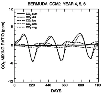
shows the model predictions for Bermuda and the infrequent yet real instances where parcels of CO2-depleted air are arriving at Bermuda during summer clearly stand out.

Therefore the model is capturing these high frequency

variations that exist in the experimental data. Also note the 'positive' outliers in the data, mostly in fall and winter, and model predictions that represent the short timescale advection

of 'polluted' air parcels from the industrialized regions of North America. This kind of detailed analysis of the model performance highlights the importance of using short timescale transport information (hours) in order to interpret certain

aspects of the observational record.

Table 2. Comparison of Seasonal Cycle Amplitudes in the Three-Dimensional Model With Observations

Site Latitude Longitude Elevation, m Model Observed

Alert, 82 ¸ 272q 62 ¸ 3 l'W 210 17.45 15.34

Ascension Island 7 ¸ 55'S 14 ¸ 25'W 54 2.51 2.25

St. Croix, Virgin Islands 17 ¸ 452q 64 ¸ 45 W 3 6.60 7.46 Azores (Terceira Island) 38 ¸ 452q 27 ¸ 05'W 30 12.11 12.72

Bermuda (east) 32 ¸ 222q 64 ¸ 39'.W 30 10.22 10.99

Bermuda (west) 32 ¸ 162q 65 ¸ 53'W 30 10.22 12.20

Point Barrow, Alaska 71 ¸ 19N 156 ¸ 36'W 30 20.20 17.40

Cold Bay, Alaska 55 ¸ 122q 162 ¸ 43'W 25 17.31 16.52 Cape Grim, Tasmania 40 ¸ 41'S 144 ¸ 41'E 94 2.29 1.15

Christmas Island 2 ¸ 002q 157 ¸ 19'W 3 2.83 3.39

Cape Meares, Oregon 45 ¸ 292q 124 ¸ 00'W 30 30.79 11.22

Guam 13 ¸ 262q 144 ¸ 47'E 2 6.26 7.79

Key Biscayne, Florida 24 ¸ 402q 80 ¸ 12'W 3 8.47 8.70

Cape Kumukahi, Hawaii 19 ¸ 312q 154 ¸ 49'W 3 9.17 8.98

Mould Bay, Canada 76 ¸ 142q 119 ¸ 20'W 15 18.07 17.27 Sand Island, Midway 28 ¸ 132q 177 ¸ 22'W 4 10.70 10.09

Mauna Loa, Hawaii 19 ¸ 322q 155 ¸ 35'W 3397 6.09 7.45

Niwot Ridge, Colorado 40 ¸ 032q 105 ¸ 38'W 3749 9.70 9.59 Palmer Station (Anvers Island) 64 ø 55'S 64 ¸ 00'W 10 3.13 2.03

Ragged Point 13 ¸ 102q 59 ¸ 26'W 3 5.98 7.62

Seychelles (Mahe Island) 4 ¸ 40'S 55 ¸ 10'E 3 3.66 2.99

Shemya Island 52 ¸ 432q 174 ¸ 06'E 40 21.74 18.99

American Samoa 14 ¸ 15'S 170 ¸ 34'W 3 1.91 1.66

Amundsen Scott (south pole) 89 ¸ 59'S 24 ¸ 48'W 2810 2.47 1.14

Ocean Station "C" 54 ¸ 002q 35 ¸ 00'W 6 17.47 14.15

Ocean Station "M" 66 ¸ 002q 2 ¸ 00'E 6 19.82 15.22

ERICKSON ET AL.' SEASONAL CYCLE OF ATMOSPHERIC CO 2 15,085 4O 30 < 20 o 10 A Model [] Observed I I Bm A [] [] -90 45 0 45 90 Latitude

Figure 3. The zonal mean of the amplitude of the seasonal cycle plotted for the 28-station model-data comparison shown

in Figure 2. Note the decreasing amplitude of the seasonal

cycle from north to south.

MAUNA LOA, HAWAII (Detrended)

358 • I ' I ' I • I ' Carbon Model ... Observed 356 _355.48 355.39 ..,-..

,•.._•__•.

'

•f/••5 354.99

-./•

354

352

6

, .

349

349.00

348.81

347 I

•

I

•

I

•

I

•

I

,

Figure 4. The detrended and smoothed seasonal cycle for 3 years from the model run and the CMDL/NOAA in situ data at Mauna Loa, Hawaii. The model results are from years 4, 5, and 6 of the model integration and the observational data are from 1989, 1990 and 1991. Note that the model and observations agree quite well with respect to the amplitude with the model underestimating the summer drawdown by about 0.7 ppm.

CCM2 MLO RESIDUALS (From Dash-dot Curve)

1994 1995

fill lilll Ill IIIIIIIIIIllllllllll I

ß .'..j.:.•4. ,.. :1

:•: 2:' ,,•..•r,•:

,. •:. : TI

,

q

,.

'....•

.P,

!

:'i

IIIIIlllllll

II Ill III;111111111111

II

1996 1997

Figure 5a. The residuals of the CCM2 model predicted

atmospheric CO2 concentrations for 3 years of model run at

Mauna Loa, Hawaii. Note that the model has a clear

seasonality in the distribution of residuals with much more

variability in the first 6 months of the year.

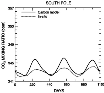
4.1.3. South Pole. Figure 9 shows the model-data compariso'ns for the seasonal cycle at the South Pole station, 90øS. Clearly from this detrended analysis, the amplitude of the model seasonal cycle is roughly a factor of 2 too large compared to the data. The phasing of the seasonal cycle data, however, is good. It is possible that the CO2 sink in the southern oceans is highly seasonal, changing the amplitude of

the annual cycle observed at the South Pole and other remote

southern hemisphere stations. It is interesting to note that the

model tendency to overestimate the seasonal cycle in the

southern hemisphere is also observed in the three-dimensional modeling study using observed winds [Keeling et al., 1989a,

b; Heimann and Keeling, 1989; Heimann et al., 1989]. In a

section below we present a detailed analysis of the individual

MAUNA LOA OBSERVATION RESIDUALS (From Smooth Curve)

3 Illlllllll IIIIIIII1111111111111111111111111111111] IIIIIIII I

2 : .-. . ,, . ... ., ß

,:.; ',,.-..., ....:,

Figure 5b. For comparison with Figure 5a the residuals of the observational atmospheric CO2 concentrations for 3 years at Mauna Loa, Hawaii. Note that the model has a similar seasonality in the residuals as the observations.

15,086

ERICKSON

ET AL' SEASONAL

CYCLE OF ATMOSPHERIC

CO2

361

f ' I ' I ' I ' I ' ' t

P -7•

355.571•

•'"•'•'56.23 -1

• • d":'• • •• • 0 356

353

8.3

i 9••

0•[.

12

13••9••••

• 352

• •8

349F

a.e.•

_•7.21

•

_•7.20

•347p•q

_[

Figure 6. The detrended and smoothed seasonal cycle for 3 years from the model run and the CMDL/NOAA flask data at

Bermuda. The model results are fi'om years 4, 5, and 6 of the model integration and the observational data are from 1989, 1990, and 1991. Note the model and observations agree quite well with respect to the amplitude of the seasonal cycle and that in the third year of the comparison the large (---5 ppm) difference between the model and the data emphasizes the climatological nature of the model forcing as contrasted with the natural variability of the real Earth system.

model component tracers that result in the model-data

differences and examine the influence of a seasonally varying

ocean source/sink formulation (MPI-Hamburg) upon the computed atmospheric seasonal cycles.

,,

I • I i I

0 220 440 660 880 1100

DAYS

Figure 8. The time series of the 12-hour model predictions for Bermuda. Note that as in Figure 7, there are a few very low

atmospheric CO2 values during the summer. This may be

interpreted as an indication that parcels of CO2-depleted air

may be advected from the North American continent to Bermuda before substantial mixing can occur. The model is

capturing this infrequent yet real atmospheric phenomena.

forcings applied [Heimann et al., 1989]. To examine this

aspect of our model, we have compared and contrasted the

model output for a sea level station, Cape Kumukahi (19.5øN,

154.8øW), with the Mauna Loa Station at 3400 m. Figures 10a

and 10b show the seasonal cycles for both the CMDL

observational data and the model output at Cape Kumukahi

and Moana Loa. The amplitude of the seasonal cycle of the

SOUTH POLE

4.2. Vertical Phasing and Amplitude of Seasonal Cycle 4.2.1. Mauna Loa and Cape Kumukahi. One of the interesting tests of model performance is how the tracer concentrations vary in the vertical in response to the surface

355 350 BERMUDA, FLASKS 370 iIiiiiiiil[11111111111[1111111111!llllllllllll[1111111111 365 o• o o o ø •5 o o 0 1990 • 99• • 992 • 993 • 994 YEAR

Figure 7. The weekly flask data of the CMDL/NOAA .group at

Bermuda. Note the very low atmospheric CO2 values that

occur once or twice a summer.

357

nE 353

Figure 9. The smoothed and detrended seasonal cycle for 3

years from the model run and the CMDL/NOAA flask data at

the south pole. The model results are from years 4, 5, and 6 of the model integration and the observational data are from 1989, 1990, and 1991. Clearly, the model overestimates the amplitude of the seasonal cycle of atmospheric CO2; however,

the phasing is quite good. We discuss the results of a

atmospheric model run using an alternative ocean forcing in a

ERICKSON ET AL.: SEASONAL CYCLE OF ATMOSPHERIC CO2 15,087

FLASK DATA

362 l ' I ' I ' I ' I [' /

r- •

Mauna

Loa,

Hawaii

•]

• ...

Cape

Kurnukah,,

Hawaii

#• j

359

..':

•

,.

,i:'

':--

352

Figure 10a. The seasonal cycle for 3 years from the

CMDL/NOAA flask data at Cape Kumukahi, Hawaii (3 m

above mean sea level (amsl)) and Mauna Loa, Hawaii (3400 m

amsl). The observational data are from 1989, 1990, and 1991.

Note that the Cape Kumukahi data always fall slightly to the left of the Mauna Loa data, indicating a phase shift of a few

weeks.

model output for Cape Kumukahi is within 0.2 part in 9 of the observed seasonal cycle (Table 2). The CMDL flask data for

Cape Kumukahi (3 m above mean sea level (amsl)) and Mauna

Loa (3400 m amsl) provide some interesting information (Figure 10a). The Cape Kumukahi observational data fall to

the left of the Mauna Loa which indicates that the lower-

elevation station experiences the terrestrial imprint on the atmospheric CO2 concentrations a few weeks before the middle

CARBON MODEL CCM2 4.809H 15.07H 32.55H 63.95H 99.04H 158.7H 189 1H 251.2H '•324 8H 408.9H 501 2H 598 2H 695 1H 786 5H 866 4H 929 2H 970,4H 992 5H Year 7

(• CO•

mixi?cj

_r?_[io

Mo•.•no

Loo,

Howoli

iDe[rent[d

o

•

Year 8 Year 9 Year 10

Figure 11. The vertical distribution of atmospheric CO2 concentration, detrended, for 3 years at the model grid point of

the Mauna Loa Observatory. Note the general decrease of the

amplitude of the seasonal cycle with increasing altitude,

except at the top of the model.

troposphere station, Mauna Loa. The amplitude of the

seasonal cycle at Cape Kumukahi is also -•25% larger than the amplitude of the seasonal cycle at Mauna Loa. Figure 10b

shows the comparison between the Cape Kumukahi Station and the Mauna Loa Station as computed by CCM2. As in the data, the Cape Kumukahi atmospheric CO2 concentrations lead the Mauna Loa concentrations by a few weeks. Also, the amplitude of the seasonal cycle is -35% larger at the lower- elevation station, in the same sense as the the observational data. The model is representing the vertical attenuation of the impact of surface forcing quite well. Figure 11 shows the time evolution over 3 model years of the vertical CO2 concentration, detrended, for the location of the Mauna Loa Observatory. Note the decrease in amplitude with increasing altitude with a small increase in seasonality at the top of the

model domain.

24 ' I ' I ' I

Mauna Loa, Hawaii Cape Kumukahi, Hawaii

E 18

t

,!4•

•,

•'"' •.

,.

12

, • • •..."..

..,': ,

..v

,:

10

z

ø

i

.,:...

, , ... 1

0

0

¸ -5

Figure 10b. The seasonal cycle for 3 years from the NCAR

CCM2 at Cape Kumukahi, Hawaii (3 m amsl) and Mauna Loa,

Hawaii (3400 m amsl). For comparison with Figure 10a, note -15 that the Cape Kumukahi model predictions always fall slightly

to the left of the Mauna Loa model predictions, similar to the observational data.

4.2.2. Sendal, Japan. We have examined the vertical attenuation of the seasonal cycle of CO2 over Sendal, Japan

(38øN, 140øE). Figures 12a and 12b show the detrended

model seasonal cycle for 3 years at -930 mbar and -410 mbar.

•SENDAI

929.21-;.I

I

-- 7.47 _-

_- 6.02

6.87

_

- 15.88 -

Figure 12a. The detrended

model seasonal

cycle of

atmospheric

CO2 at the model

surface

level for Sendal,

Japan.

15,088

_ERICKSON

_{ET AL.: SEASONAL}

_{CYCLE OF ATMOSPHERIC}

_CO2

SENDAl 408.9H CAPE GRIM, TASMANIA-AUSTRALIA 408.9H

4

2

.

-4

Year

4

Year

5

Year

6

Year

7

Year

4

Year

5

Year

6

Year

7

Figure

12b. The detrended

model

seasonal

cycle

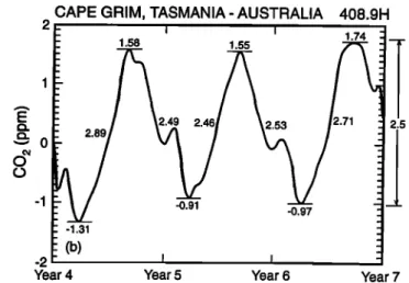
of Figure

13b.

The

detrended

seasonal

cycle

of

atmospheric

CO2

atmospheric

CO2

at

the

--410-mbar

level

for

Sendal,

Japan.

The at the

-•410

mbar

level

for

Cape

Grim,

Tasmania

The

mean

mean

amplitude

of the

seasonal

cycle

is -•8.4

ppm

CO2,

roughly

amplitude

of the

seasonal

cycle

is -•2.5

ppm

CO2,

roughly

20%

a factor

of 2 less

than

at

the

surface

(Figure

12a).

greater

than

at the

surface,

Figure

13a.

The

amplitude

of atmospheric

CO2 at the surface

is roughly

16.6 ppm. The small 'shoulders' during the first few months of

the

year

are

due

to transport

processes

in the boundary

layer

interacting

with the surface

emission

patterns.

Figure 12b

shows the detrended seasonal cycle at --410 mbar. The

amplitude

of the seasonal

cycle

in atmospheric

CO2

is 8.4 ppm,

comparison with some observational data, Tanaka et al. [ 1987], report seasonal cycle amplitudes in the lowest 2 km of the atmosphere of---14.2 ppm and 8.0 ppm at ---410 mbar. This

indicates

that the boundary

layer proccesses

are working

Pacific, as indicated by the analysis for Mauna Loa.

4.2.3. Cape Grim, Tasmania. The seasonal

cycle

in the

southern

hemisphere

has

been

seen

to be substantially

smaller

and models.

At Cape

Grim,

Tasmania

(40øS,

144øE),

Figures

13a and 13b show the derrended

model

amplitudes

for two

-2

CAPE GRIM, TASMANIA- AUSTRALIA 929.2H

1.8••-•

I 1.85

I 1.99

•

• -0.13

-0.35

.05

(a)

I

I

Figure 13a. The detrended

seasonal

cycle

of atmospheric

CO2

at the model surface level for Cape Grim, Tasmania. The mean

amplitude of the seasonal cycle is ---2.1 ppm CO2.

show the seasonal cycle at the surface to be roughly 2.1 ppm, whereas at 410 mbar it is actually larger by ---20%, 2.5 ppm.

This is exactly opposite what is observed and modeled at the northern hemisphere sites. This is due to the fact that the

transport of northern hemisphere CO2 to the southern hemisphere occurs most efficiently in the middle troposphere,

an aspect verified by observational data [Pearman and

Beardsmore, 1984] and replicated in the modeling study of

Keeling et al. (1989a, b).

4.3. Interhemispheric gradient. The interhemispheric

gradient of atmospheric CO2 is closely linked to the

magnitude and spatial distributions of the surface source/sink

terms. To first order, the large--5.3 Gt C (as CO2) source to the atmosphere from the combustion of fossil fuels occurs primarily in the northern hemisphere and one would expect the northern

hemisphere annual mean CO2 mixing ratio to be higher than

the southern hemisphere. However, this expectation should

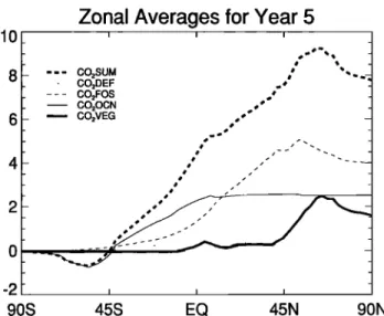
ZONAL AVERAGES FOR YEARS 4, 5, 6

13 , • , • , • , 12 - -180 to -90 , I \ 11 ... 90 to 0 • • -

•' 10

Oto90

'

•'

-

90 to 180

] /'" \

•

7

/

'

•

6

0

..•

,/

-

Figure 14. •c zonal average

of the a•osphcdc CO

2