Morphing wing real time optimization in wind tunnel tests

Publisher’s version / Version de l'éditeur:

Proceedings of the 7th International Conference on Informatics in Control,

Automation and Robotics, Funchal, Madeira, Portugal, June 15-18, 2010, 1,

Inteligent control systems and optimization, 2010

READ THESE TERMS AND CONDITIONS CAREFULLY BEFORE USING THIS WEBSITE.

https://nrc-publications.canada.ca/eng/copyright

Vous avez des questions? Nous pouvons vous aider. Pour communiquer directement avec un auteur, consultez la première page de la revue dans laquelle son article a été publié afin de trouver ses coordonnées. Si vous n’arrivez pas à les repérer, communiquez avec nous à PublicationsArchive-ArchivesPublications@nrc-cnrc.gc.ca.

Questions? Contact the NRC Publications Archive team at

PublicationsArchive-ArchivesPublications@nrc-cnrc.gc.ca. If you wish to email the authors directly, please see the first page of the publication for their contact information.

NRC Publications Archive

Archives des publications du CNRC

This publication could be one of several versions: author’s original, accepted manuscript or the publisher’s version. / La version de cette publication peut être l’une des suivantes : la version prépublication de l’auteur, la version acceptée du manuscrit ou la version de l’éditeur.

Access and use of this website and the material on it are subject to the Terms and Conditions set forth at

Morphing wing real time optimization in wind tunnel tests

Popov, Andrei Vladimir; Grigorie, Teodor lucian; Botez, Ruxandra Mihaela;

Mamou, Mahmoud; Mebarki, Youssef

https://publications-cnrc.canada.ca/fra/droits

L’accès à ce site Web et l’utilisation de son contenu sont assujettis aux conditions présentées dans le site LISEZ CES CONDITIONS ATTENTIVEMENT AVANT D’UTILISER CE SITE WEB.

NRC Publications Record / Notice d'Archives des publications de CNRC:

1

Real Time Morphing Wing Optimization in a Wind Tunnel

Andrei V. Popov1 _{, Lucian T. Grigorie.}2_{, Ruxandra Mihaela Botez}3

École de Technologie Supérieure, Montréal, Québec, H3C 1K3

Mahmoud Mamou4_{, Youssef Mébarki}5

Institute for Aerospace Research, NRC, Ottawa, Ontario, K1A 0R6, Canada

In this paper, wind tunnel results of a real time optimization of a morphing wing in wind tunnel for delaying the transition towards the trailing edge are presented. A morphing rectangular finite aspect ratio wing, having a WTEA reference airfoil cross-section, was considered with its upper surface made of a flexible composite material and instrumented with Kulite pressure sensors, and two smart memory alloys actuators. Several wind tunnel tests runs for various Mach numbers, angles of attack and Reynolds numbers were performed in the 6’×9’ wind tunnel at the Institute for Aerospace Research at the National Research Council Canada (IAR/NRC). Unsteady pressure signals were recorded and used as feed back in real time control while the morphing wing was requested to reproduce various optimized airfoils by changing automatically the two actuators strokes. The paper shows the optimization method implemented into the control software code that allows the morphing wing to adjust its shape to an optimum configuration under the wind tunnel airflow conditions.

Nomenclature

α = angle of attack of the wing

b = span of wing model

c = chord of wing airfoil

Cp = pressure coefficient

CRIAQ = Consortium for Research and Innovation in Aerospace in Quebec ETS = Ecole de Technologie Superieure

FFT = Fast Fourier Transform

IAR-NRC = Institute for Aerospace Research - National Research Council Canada LVDT = Linear Variable Differential Transducer

M = Mach number

Re = Reynolds number

RMS = Root Mean Square

SMA = Shape Memory Alloy

1 _{PhD student, Laboratory of Research in Active Controls, Avionics and AeroServoElasticity LARCASE, 1100}

Notre-Dame West Street, Montreal, Quebec, H3C 1K3, Canada, AIAA Member.

2 _{Post-Doc fellowship, Laboratory of Research in Active Controls, Avionics and AeroServoElasticity LARCASE,}

1100 Notre-Dame West Street, Montreal, Quebec, H3C 1K3, Canada, AIAA Member.

3 _{Corresponding Author, Professor, Laboratory of Research in Active Controls, Avionics and AeroServoElasticity}

LARCASE, www.larcase.etsmtl.ca, 1100 Notre-Dame West Street, Montreal, Quebec, H3C 1K3, Canada, AIAA Member.

4 _{Senior Research Officer, Aerodynamics Laboratory, Institute for Aerospace Research, National Research Council,}

Montreal Road, Uplands Bldg. U66, Ottawa, Ontario, K1A 0R6, Canada, AIAA Member.

5 _{Associate Research Officer, Aerodynamics Laboratory, Institute for Aerospace Research, National Research}

I.

Introduction

he CRIAQ 7.1 project is a collaborative project between the teams from École de technologie superieure (ETS), École Polytechnique, the Institute for Aerospace Research - National Research Canada (IAR-NRC), Bombardier Aerospace, Thales Avionics. In this project, the laminar flow past aerodynamically morphing wing is improved in order to obtain important drag reductions.

This collaboration calls for both aerodynamic modeling as well as conceptual demonstration of the morphing principle on real models placed inside the wind tunnel. Drag reduction on a wing can be achieved by modifications of the airfoil shape which has an effect in the laminar flow to turbulent flow transition point position, which should move toward the trailing edge of the airfoil wing. The main objective of this concept is to promote large laminar regions on the wing surface, thus reducing drag over an operating range of flow conditions characterized by Mach numbers, airspeeds and angles of attack [1]. The airborne modification of an aircraft wing airfoil shape can be realized continuously to maintain laminar flow over the wing surface as flight conditions change. To achieve such a full operating concept, a closed loop control system concept was developed by us to control the flow fluctuations over the wing surface with the deformation mechanisms (actuators) [2].

The wing model has a rectangular plan form of aspect ratio of 2 and is equipped with a flexible upper surface skin on which shape memory alloys actuators are installed. Two shape memory alloys actuators (SMA) create the displacement of the two control points on the flexible skin in order to realize the optimized airfoil shapes.

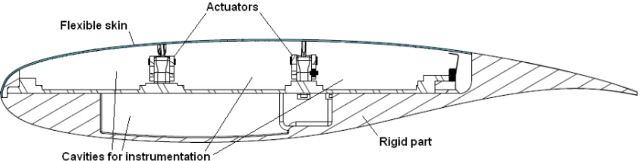
Figure 1. Cross section of the morphing wing model

As reference airfoil, a laminar airfoil WTEA was used; its aerodynamic performance was investigated at IAR-NRC in refs. [3, 4], and the optimized airfoils were previously calculated by modifying the reference airfoil for each airflow condition as combinations of angles of attack and Mach numbers such that the transition point position was found to be the nearest as possible to the airfoil trailing edge. Several optimized airfoils were found for the airflow cases combinations of Mach numbers and angles of attack. The optimized airfoils configurations are stored in the computer memory by means of a database and are selected as needed by the operator or computer in order to be realized by the morphing wing. But this strategy relies on the previously calculated aerodynamical characteristics of the airfoils which usually are determined by use of CFD codes and optimization algorithms. The idea presented in this paper is to implement the same optimization algorithm into the computer controller that will search the optimal configuration with the real system, in real time and in real aerodynamical airflow conditions.

II.

Experimental setup description

A. Mechanical and electrical control system

The concept of this morphing wing consisted in a rectangular wing model (chord c = 0.5 m and span b = 2.1 m) incorporating two parts. One fixed part was built in aluminum by the IAR-NRC team and sustained the resistance forces acting during wind tunnel tests. The other part was flexible consisted in its flexible skin installed on the wing upper surface and was designed and manufactured at ETS (Fig. 1). The flexible skin was required to change its shape through two action points in order to realize the optimized airfoil for the airflow conditions in which tests were performed.

The actuators were composed of two oblique cams sliding rods span-wise positioned that converted the horizontal movement along the span in vertical motion perpendicular to the chord (Fig. 2). The position of each actuator was given by the mechanical equilibrium between the Ni-Ti alloy SMA wires that pulled the sliding rod in

3

one direction and the gas springs that pulled the sliding rod in the reverse direction. The gas springs role was to counteract the pulling effect of aerodynamical forces acting in wind tunnel over the flexible skin when the SMA’s were inactive. Each sliding rod was actuated by means of three parallel SMA wires connected to a current controllable power supply which was the equivalent of six wires acting together. The pulling action of the gas spring retracted the flexible skin in the undeformed-reference airfoil position, while the pulling action of the SMA wires deployed the actuators in the load mode i.e. morphed airfoil in the optimized airfoil position (see Fig. 2). The gas springs used for these tests were charged with an initial load of 225 lbf (1000 N) and had a characteristic rigidity of 16.8 lbf / in (2.96 N / mm). x z flexible skin spring SMA actuator rod roller cam First actuating line Second actuating line

Figure 2. Schematics of the flexible skin mechanical actuation

The mechanical SMA actuators system is controlled electrically through an “open loop” control system. The architecture of the wing model open loop control system, SMA actuators and controller is shown in Figure 3. The two SMA actuators have six wires each, which are supplied with power by the two AMREL SPS power supplies, controlled through analog signals by the NI-DAQ USB 6229 data acquisition card. The NI-DAQ is connected to a laptop through an USB connection. A control program is implemented in Simulink which provides to the power supplies the needed SMA current values through an analog signal as shown in Figure 3. The control signal of 2 V corresponds to a SMA supplied current of 33 A. The Simulink control program uses as feedback three temperature signals coming from three thermocouples installed on each wire of the SMA actuator, and a position signal from a LVDT sensor connected to the oblique cam sliding rod of each actuator. The temperature signals serve in the overheat protection system that disconnect the current supply to the SMA in case of wire temperature pass over the set limit of 120°C. The position signals serve as feedback for the actuator desired position control. The oblique cam sliding rod has a horizontal versus vertical ratio 3:1; hence the maximum horizontal displacement of the sliding rod by 24 mm is converted into a maximum vertical displacement of the actuator and implicit of the flexible skin by 8 mm.

A user interface is implemented in Matlab/Simulink which allows the user to choose the optimized airfoils shape from database stored on the computer hard disk and provides to the controller the vertical needed displacements in order to obtain the desired optimized airfoil shape. The controller activates the power supplies with the needed SMA current values through an analog signal as shown in Figure 3. The control signal of 2 V corresponds to a SMA supplied current of 33 A. In practice, the SMA wires were heated at an approximate temperature of 90°C with a current of 10 A. When the actuator reached the desired position the current was shut off and the SMA was cycled in endless heating/cooling cycles through the controller switching command on/off of the current in order to maintain the current position until another desired position or the entire system shut off was required.

In support of the discrete pressure instrumentation, infrared thermography (IR) visualization was performed to detect the transition location on the morphing wing upper surface and validate the pressure sensor analysis. The transition detection method using IR is based on the differences in laminar and turbulent convective heat transfer coefficient and was exacerbated by the artificial increase of model-air flow temperature differences. In the resulting images, the sharp temperature gradient separating high temperature (white intensity in image) and low temperature (dark intensity) regions is an indication of the transition location. The infrared camera used was an Agema SC3000 camera, equipped with a 240×320 pixels QWIP detector, operating in the infrared wavelength region of 8-9 m and cooled to 70°K to reduce thermal noise. The camera provided a resolution of 0.02°C and a maximum frame rate of 60 Hz. It was equipped with the default lens (FOV = 20°×15°), and was installed 1.5 m away from the model with an optical axis oriented in the horizontal plane at about 30° with respect to the wing surface mid-chord normal. Optical access was provided through an opening on the side wall of the test section opposite to the upper surface. More details about the methodology and processing are available in [REFX].

B. Aerodynamical detection system and graphical user interface

The morphing wing goal is the improvement of the laminar flow over the upper surface of the wing. In order to ensure that the improvement is real, we built a detection system that gives information about the flow characteristics. An array of twelve Kulite pressure sensors was installed on the flexible skin.

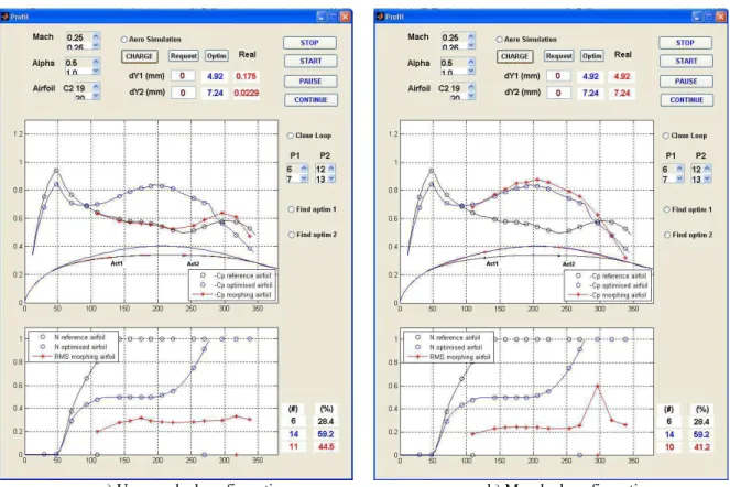
The pressure data acquisition was performed using a NI-DAQ USB 6210 card with 16 analog inputs, at a total sampling rate of 250 kS/s. The input channels were connected directly to the IAR-NRC analog data acquisition system which was connected to the twelve Kulite sensors. The IAR-NRC served as an amplifier and conditioner of the signal at a sampling rate of 15 kS/s. One extra channel was used for the wind tunnel dynamic pressure acquisition to calculate the pressure coefficients Cp’s from the pressure values measured by the twelve pressure sensors. The signal was acquisitioned at sampling rate of 10 kS/s in frames of 1024 points for each channel which allowed a boundary layer pressure fluctuations FFT spectral decomposition up to 5 kHz for all channels, at a rate of 0.1024 Samples/s using Matlab/Simulink software. The plot results were visualized in real time on the computer screen in dedicated windows (see Figure 4) at a rate of 1.024 Samples/sec. Figure 4 shows an example of graphical user interface in which all the aerodynamical and morphing shape information were centralized together with the control buttons of the controlling software. The window shows information about the Mach number, the angle of attack, the airfoil shape of the morphing wing, and the two actuators vertical displacements needed to obtain the desired airfoil shape. In the two plots, are shown the coefficients pressure distribution Cp’s of the twelve Kulite sensors, and the noise of the signal (RMS) of each pressure signal. Left figure shows the wing un-morphed position, while the right figure shows the wing under its morphed position. The results obtained are qualitatively very similar to those obtained in previous studies [5].

5

a) Un-morphed configuration b) Morphed configuration

Figure 4. Graphical User Interface (GUI) where all the aerodynamical and morphing shape information are centralized together with the control buttons of the software.

The transition between laminar and turbulent flow is detected by means of each pressure signal’s RMS. The lowest RMS plot given in Figure 4 shows the quantity of the pressure signal noise from each Kulite sensor (red star curve). In the example shown in Figures 4, the RMS red plot in the un-morphed configuration (Figure 4.a) does not show any transition due to the fact that all twelve sensors show the turbulent flow.

In Figure 4.a, on the GUI is shown an un-morphed airfoil by use of a black colour. The actuators reference positions correspond to dY1 = 0 mm and dY2 = 0 mm, the Cp distribution calculated by XFoil for the reference airfoil (black curve), and the Cp theoretical values of the sensors shown as black circles on the Cp distribution curve.

In the lower plot of Figure 4.a is shown the N factor used by Xfoil to predict transition for the reference airfoil (black curve). In the case of an un-morphed configuration, the predicted transition position is found to be the 6th

position of the sixteen available sensors positions. In the beginning of wind-tunnel tests, a number of sixteen sensors were installed, but due to their removal and re-installation during the next two wind tunnel tests, four of them were found defective, therefore a number of twelve sensors remained to be used during the last third wind tunnel tests so only twelve Kulite sensors were used for plotting the Cp distribution and RMS distribution (red star plots).

Results predicted for the morphed airfoil are shown in blue color. The morphed airfoil coordinates are shown as blue curves in the upper part of Figure 4.b, the Cp distribution is calculated by XFoil for the optimized airfoil (blue curve), and the Cp theoretical values of the sensors are shown as blue circles on the Cp distribution curve. In the lower plot of Figure 4.b, the N factor used by Xfoil to predict transition is shown for the optimized airfoil (blue curve). In this case of morphed configuration, the predicted position of transition is the 14th _{position of the sixteen}

available sensors positions.

These black (un-morphed) and blue (morphed) curves serve as theoretical validations of the red curves reflecting the aerodynamic parameters (Cp and RMS) provided by Kulite sensors in real time with a sampling rate of 1 S/sec. In Figure 4.b is shown the actuated airfoil in the morphed position (dY1 = 4.92 mm and dY2 = 7.24 mm). The transition position is given by the sensor location where the maximum RMS is found, which in this case is the 10th _{Kulite sensor out of 12 sensors. The instant visualization allows us to find the exact position predicted by XFoil.}

III.

Simulation and Experimental results obtained in the wind tunnel

A. Optimization control

The basic idea of optimization control is to by-pass the necessity of a previously calculated optimized airfoils database, and to generate in real time the optimized airfoil for the exact conditions of the wind flow. For such a task it is necessary to develop a subroutine that optimizes the airfoil shape in the same way the optimized airfoils database was generated. The method of optimization used in this case is a mixed method between ‘the gradient ascent’ or ‘hill climbing’ method and the ‘simulated annealing’ which is a meta-heuristic search method. The reason why is needed a mixed method is that the cost function for such complex problem (minimize the CD, maximize the

CL/CD or maximize the transition point position xtr for a morphing wing) is not defined analytically and the implementation of ‘gradient ascent’ method is not suitable. Also, due to time cost (very long time response of the SMA actuators due to heating but especially cooling time) a purely probabilistic meta heuristic search algorithm is not suitable too. The mixed method that was found to be the quickest and in the same time most accurate for finding the transition point position xtr maximum is shown in the following paragraph.

The simulation of the system used as platform was the Matlab/Simulink software. The simulation used the optimization subroutine exactly the same as in bench tests and wind tunnel tests, except that in computer simulation and bench test the aerodynamical pressures that action upon the skin and stimulates the sensors were simulate by use of XFoil software. As mathematical model of the flexible skin was used a B-spline with four flexion points. Two points were fixed where the skin is glued on the wing rigid structure and two points were mobile and are placed in the actuators coordinates on the wing structure. The B-spline shape that define the airfoil’s flexible skin does not have the same coordinates as the flexible skin but is a good approximation for the purpose of designing an optimization subroutine in closed loop with a CFD code. The logic schematic of the optimization subroutine is shown in Fig. 8.

Figure 5. Optimization logic schematic B. Simulation and experiment results compared

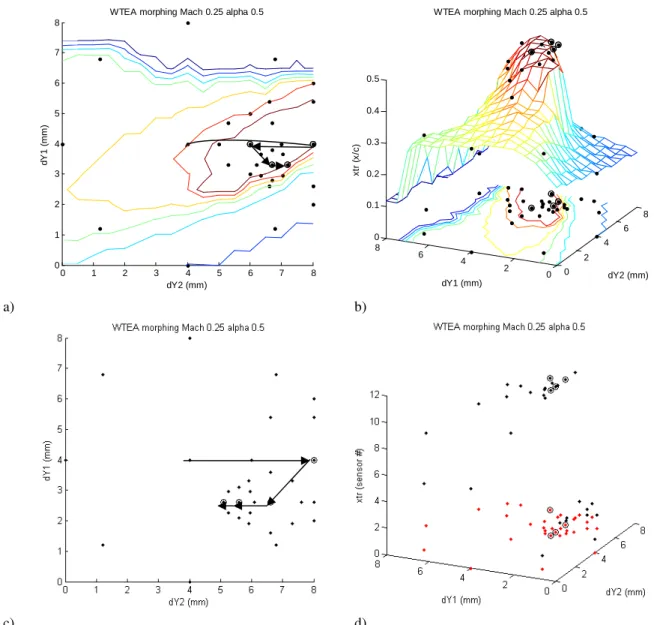
The domain in which the optimizer search the best configuration is defined by the bi-dimensional space of actuators strokes {dY1 = [0, 8], dY2 = [0, 8]}. The initial point of the optimizer is defined as dY1 = 4 mm and dY2 = 4 mm. Then the first round of evaluation points consist of eight points situated in a circle with the ray of 4 mm around the initial point. For each evaluation point, the xtr value is evaluated by use of XFoil and stored in the

memory. After the first round of evaluations the optimizer decides which evaluating point had the maximum value of xtr, which will became the initial point for the next round of evaluations. Figures 6.a, 6.b and 7 show the result of

WTEA airfoil optimization after four evaluation rounds, first evaluation with a radius of 4 mm, second evaluation with a radius of 2 mm, third evaluation with a radius of 1 mm and fourth and last evaluation with a radius of 0.5 mm. As seen in Figure 6.b the last round of evaluation is almost unnecessary because the maximum xtr is found

inside a plateau of maximums with very small differences between them. Before doing the optimization it was performed a mapping of the search domain, i.e. for each combination of dY1 and dY2 in the interval [0 mm, 8 mm] with a step of 1 mm it was found the xtr and was built the surface xtr = f (dY1,dY2). Figure 6.c and 6.d show the

same optimization routine that run during the wind tunnel tests in the same airflow conditions as the ones simulated except that there is no map of the searched function. The result is slightly different because the airfoil shape of the real flexible skin under wind tunnel conditions is different than the airfoil shapes defined by use of B-splines. Still the result is similar, in terms of actuator strokes dY1 and dY2 as well as the position of transition. Similarly there can be observed in Figure 6.d a plateau of evaluation points that had the transition occurrence on the 11th _sensor.

7 0 1 2 3 4 5 6 7 8 0 1 2 3 4 5 6 7 8

WTEA morphing Mach 0.25 alpha 0.5

dY2 (mm) d Y 1 ( m m ) 0 2 4 6 8 0 2 4 6 8 0 0.1 0.2 0.3 0.4 0.5 dY2 (mm) WTEA morphing Mach 0.25 alpha 0.5

dY1 (mm) x tr ( x /c ) a) b) c) d)

Figure 6. Optimization in simulation using XFoil code a) and b) vs. optimization in real time during wind tunnel tests c) and d) for the same airflow conditions M = 0.25 and αααα = 0.5°.

Figure 7 shows the optimization result airfoil shape, Cp distribution and xtr transition point position on the upper surface of the airfoil obtained through simulation using XFoil and B-splines model for the flexible skin. The values obtained for wind flow conditions of Mach = 0.25 and a = 0.5 are dY1 = 3.3 mm and dY2 = 7.2 mm. Also in Figure 7 is shown the N factor distribution which is the parameter used by XFoil to calculate the transition point position. When N factor reaches the Ncr critical value the transition is triggered. This parameter was used in wind tunnel to

validate the transition position found through the RMS measuring of the Kulite pressure sensors.

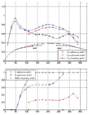
Figure 8 shows the optimization airfoil shape, Cp distribution and xtr transition point position on the upper surface of the airfoil in wind tunnel test (red plots) compared to the optimal airfoil plots (blue) and reference airfoil plots (black) obtained through simulation. Also in the lower subplot of Figure 8 the N factor used by XFoil to detect the transition position is compared to the RMS of the Kulite sensors. Both the N factor and RMS are normalized and the purpose of the plots is to have a visual indicator of the transition position. The software considers the transition position in the coordinates of the sensor with the highest noise (RMS) as confirmed by previous studies [5].

0 0.1 0.2 0.3 0.4 0.5 0.6 0.7 0.8 0.9 1 -0.6 -0.4 -0.2 0 0.2 0.4 0.6 0.8 1 1.2 1.4

WTEA morphing Mach 0.25 alpha 0.5

x/c

-C

p

-Cp reference airfoil -Cp morphing airfoil N factor reference airfoil N factor morphing airfoil x_tr reference airfoil

x_tr morphing airfoil

Figure 7. Optimization simulation result of xtr = 0.497 for dY1 = 3.3 mm and dY2 = 7.2 mm

Figure 8. Optimization result of xtr /c = 0.635 (xtr =317.5 mm) for dY1 = 2.6 mm and dY2 = 5.1 mm during

wind tunnel test for M = 0.25 and αααα = 0.5°

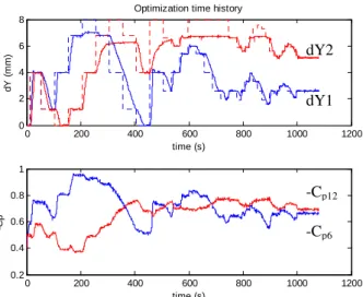
Figure 9 shows the time history of the optimization process in wind tunnel. Due to the long response of the SMA actuators – the time of cooling from maximum displacement to zero was approx 2 min – the entire process of optimum search converged to the optimum values in approx 20 min. Also, there can be observed that the requested displacements of the actuators at the maximum displacement of 8 mm were not realized, due to the fatigue of the SMA’s accumulated in previous testes. The maximum deflection was in fact 7 mm for the first actuator and 6.5 mm for second actuator which could not physically be passed over.

9 0 200 400 600 800 1000 1200 0 2 4 6 8 time (s) d Y ( m m )

Optimization time history

0 200 400 600 800 1000 1200 0.2 0.4 0.6 0.8 1 time (s) -C p

Figure 9. Optimization time history during wind tunnel test for M = 0.25 and αααα = 0.5°

Figure 10 shows typical infrared results obtained at M = 0.25, α = 0.5° for various configurations. Only the composite portion of the wing at x/c≤0.7 is shown. The white spots on the wing are the electronically heated Kulite pressure transducers. The two lines of SMA actuators, colder than the model surface, are also visible at quarter chord and near mid-chord. The locations of the transition in the images have been highlighted using a white dashed line: it corresponds to the location of a large surface temperature gradient, the laminar region being about 2-3°C hotter than the turbulent region. The reference airfoil configuration (Figure 10-a) showed a transition location at x/c = 26%. The optimization (Figure 10-b) allowed a laminar boundary layer run to x/c = 58%, which represents a significant improvement over the reference case (Figure 10-a). Some turbulent wedges caused by leading edge contamination, due to dust particles in the flow, are visible in Figure 10-a. In addition to providing an on line verification of the Kulite dynamic pressure signals, the infrared measurement was particularly useful to detect those early artificial turbulent regions. When the level of contamination was estimated unacceptable or likely to affect the drag or the Kulite measurements, the test was interrupted and the model was carefully cleaned.

a) b)

Figure 10. Infrared results obtained at M = 0.25 and αααα = 0.5° in a) Reference, b) After optimization

dY1 dY2 -Cp12 -Cp6 Turbulent wedges

IV.

Conclusions

The results of the tests performed in wind tunnel using a morphing wing were shown. The optimization method does not use any CFD code but use the same optimization algorithm in real time. This optimization converges in approximately 10 minutes due to the slow response of the SMA actuators especially in the cooling phase of the cycle. It was observed that the airfoil realized by this method slightly differs from the optimization using CFD codes. This result was due to the fact that the cost function of the optimization (transition position) has discrete values (the sensors positions) and the maximum of the function is a plateau of different dY1 and dY2 values. The optimizer stops at a certain value in function of the number and magnitudes of the searching steps. It was observed that the last searching step (searching of the maximum in eight points situated on a circle with ray of 0.5 mm – see Figure 9) is not necessary due to the cost function plateau of maximums.

Acknowledgments

The authors would like to thank the Consortium of Research in the Aerospatial Industry in Quebec (CRIAQ) and to the NSERC for funding the present work, and Thales Avionics and Bombardier Aerospace for their financial and technical support. The authors would like also to thank George Henri Simon for initiating CRIAQ 7.1 project, to Eric Laurendeau from Bombardier Aerospace and to Philippe Molaret from Thales Avionics for their collaboration on this work.

References

[1] Zingg, D. W., Diosady, L., and Billing, L., “Adaptive Airfoils for Drag Reduction at Transonic Speeds,” AIAA paper 2006-3656, 2006.

[2] Popov. A-V., Labib, M., Fays, J., Botez, R.M., 2008, Closed loop control simulations on a morphing laminar

airfoil using shape memory alloys actuators, AIAA Journal of Aircraft, Vol. 45(5), pp. 1794-

[3] Khalid, M., Navier Stokes Investigation of Blunt Trailing Edge Airfoils using O-Grids, AIAA Journal of Aircraft, 1993.

[4] Khalid, M., and Jones, D.J., A CFD Investigation of the Blunt Trailing Edge Airfoils in Transonic Flow, Inaugural Conference of the CFD Society of Canada (June 1993).

[5] Nitcshe, W., Mirow, P., Dorfler, T., Investigations on Flow Instabilities on Airfoils by Means of Piezofoil –

Arrays, Laminar-Turbulent Transition IUTAM Symposium, Toulouse, France, 1989.

[6] Popov, A-V., Botez, R. M., and Grigorie, L., Morphing Wing Validation during Bench Tests, 2009 Canadian Aeronautics and Space Institute Annual General Meeting, Aircraft Design & Development Symposium, Kanata, Ontario 2009.

[7] Y. Mébarki, M. Mamou and M. Genest, Infrared Measurements of Transition Location on the CRIAQ project