from New and Used Car Purchases
The MIT Faculty has made this article openly available.
Please share
how this access benefits you. Your story matters.
Citation
Busse, Meghan R, Christopher R Knittel, and Florian Zettelmeyer.
“Are Consumers Myopic? Evidence from New and Used Car
Purchases.” American Economic Review 103, no. 1 (February 2013):
220–256. © 2013 by the American Economic Association.
As Published
http://dx.doi.org/10.1257/aer.103.1.220
Publisher
American Economic Association
Version
Final published version
Citable link
http://hdl.handle.net/1721.1/87769
Terms of Use
Article is made available in accordance with the publisher's
policy and may be subject to US copyright law. Please refer to the
publisher's site for terms of use.
220
Are Consumers Myopic?
Evidence from New and Used Car Purchases
†By Meghan R. Busse, Christopher R. Knittel,
and Florian Zettelmeyer*
We investigate whether car buyers are myopic about future fuel costs. We estimate the effect of gasoline prices on short-run equilib-rium prices of cars of different fuel economies. We then compare the implied changes in willingness-to-pay to the associated changes in expected future gasoline costs for cars of different fuel economies in order to calculate implicit discount rates. Using different assump-tions about annual mileage, survival rates, and demand elasticities,
we calculate a range of implicit discount rates similar to the range of interest rates paid by car buyers who borrow. We interpret this as showing little evidence of consumer myopia. (JEL D12, H25, L11,
L62, L71, L81)
According to Environmental Protection Agency (EPA) estimates, gasoline
combustion by passenger cars and light-duty trucks is the source of about 15 percent of US greenhouse gas emissions, “the largest share of any end-use
eco-nomic sector.”1 As public concerns about climate change grow, so does interest in
designing policy instruments that will reduce carbon emissions from this source. In order to be effective, any such policy must reduce gasoline consumption, since carbon emissions are essentially proportional to the amount of gasoline used. The major policy instrument that has been used so far to influence gasoline con-sumption in the United States has been the Corporate Average Fuel Efficiency (CAFE) standards (Goldberg 1998, Jacobsen 2010). Some economists, however, contend that changing the incentives to use gasoline—by increasing its price—
1 EPA, Inventory of US Greenhouse Gas Emissions and Sinks: 1990–2006, p. 3–8.
* Busse: Kellogg School of Management, Northwestern University, 2001 Sheridan Road, Evanston, IL 60208, and NBER (e-mail: [email protected]); Knittel: MIT Sloan School of Management, 100 Main Street, Cambridge, MA 02142, and NBER (e-mail: [email protected]); Zettelmeyer: Kellogg School of Management, Northwestern University, 2001 Sheridan Road, Evanston, IL 60208, and NBER (e-mail: f-zettelmeyer@kellogg. northwestern.edu). We are grateful for helpful comments from Hunt Allcott, Eric Anderson, John Asker, Max Auffhammer, Severin Borenstein, Tim Bresnahan, Igal Hendel, Ryan Kellogg, Aviv Nevo, Sergio Rebelo, Jorge Silva-Risso, Scott Stern, and three anonymous referees. We thank seminar participants at Brigham Young University, the Chicago Federal Reserve Bank, Cornell, Harvard, Illinois Institute of Technology, Iowa State, MIT, Northwestern, Ohio State, Purdue, Texas A&M, Triangle Resource and Environmental Economics seminar, University of California Berkeley, University of California Irvine, University of British Columbia, University of Chicago, University of Michigan, University of Rochester, University of Toronto, and Yale. We also thank partici-pants at the ASSA, Milton Friedman Institute Price Dynamics Conference, NBER IO, EEE, and Price Dynamics conferences, and the National Tax Association. We thank the University of California Energy Institute (UCEI) for financial help in acquiring data. Busse and Zettelmeyer gratefully acknowledge the support of NSF grants SES-0550508 and SES-0550911. Knittel thanks the Institute of Transportation Studies at UC Davis for support.
would be a preferable approach. This is because changing the price of gasoline has the potential to influence both what cars people buy and how much people drive.
This article addresses a question that is crucial for assessing whether a gasoline
price related policy instrument (such as an increased gasoline tax or a carbon tax)
could influence what cars people buy: how sensitive are consumers to expected future gasoline costs when they make new car purchases? More precisely, how much does an increase in the price of gasoline affect the willingness-to-pay of consumers for cars of different fuel economies? If consumers are very myopic, meaning that their willingness-to-pay for a car is little affected by changes in the expected future fuel costs of using that car, then a gasoline price instrument will not influence their choices very much and will not be sufficient to achieve the first-best outcome in the presence of an externality. This condition is not unique
to the case of gasoline consumption. Hausman (1979) was the first to
investi-gate whether consumers are myopic when purchasing durable goods that vary in energy costs. More generally, this is an example of the quite obvious point that a policy must influence something that consumers pay attention to in order to actu-ally affect the choices consumers make.
Our analysis proceeds in two steps. First, we estimate how the price of gaso-line affects market outcomes in both new and used car markets. Specifically, we use data on individual transactions for new and used cars to estimate the effect of gasoline prices on equilibrium transaction prices, market shares, and sales for new and used cars of different fuel economies. We find that a $1 change in the gasoline price is associated with a very large change in relative prices of used cars of different fuel economies—a difference of $1,945 in the relative price of the highest fuel economy and lowest fuel economy quartile of cars. For new cars, the predicted relative price difference is much smaller—a $354 difference between the highest and lowest fuel economy quartiles of cars. However, we find a large change in the market shares of new cars when gasoline prices change. A $1 increase in the gasoline price leads to a 21.1 percent increase in the market share of the highest fuel economy quartile of cars and a 27.1 percent decrease in the market share of the lowest fuel economy quartile of cars. These estimates become the building blocks for our next step.
In our second step, we use the estimated effect of gasoline prices on prices and quantities in new and used car markets to learn about how consumers trade off the up-front capital cost of a car and the ongoing usage cost of the car. We estimate a range of implicit discount rates under a range of assumptions about demand elasticities, vehicle miles traveled, and vehicle survival probabilities. We find little evidence that consumers “undervalue” future gasoline costs when purchasing cars. The implicit discount rates we calculate correspond reasonably closely to interest rates that customers pay when they finance their car purchases.
This article proceeds as follows. In the next section, we position this paper within the related literature. In Section II we describe the data we use for the analysis in this paper. In Section III we estimate the effect of gasoline prices on equilibrium prices, market shares, and unit sales in new and used car markets. In Section IV we use the results estimated in Section III to investigate whether consumers are myopic, meaning whether they undervalue expected future fuel
costs relative to the up-front prices of cars of different fuel economics. Section V checks the robustness of our estimated results. Section VI offers some conclud-ing remarks.
I. Related Literature
There is no single, simple answer to the question “How do gasoline prices affect gasoline usage?” and, consequently, no single, omnibus paper that answers the entire question. This is because there are many margins over which drivers, car buyers, and automobile manufacturers can adjust, each of which will ultimately affect gasoline usage. Some of these adjustments can be made quickly; others are much longer run adjustments.
For example, in the very short run, when gasoline prices change, drivers can very
quickly begin to alter how much they drive. Donna (2011), Goldberg (1998), and
Hughes, Knittel, and Sperling (2008) investigate three different measures of driving
responses to gasoline prices. Donna investigates how public transportation utiliza-tion is affected by gasoline prices, Goldberg estimates the effect of gasoline prices on vehicle miles traveled, and Hughes, Knittel, and Sperling investigate monthly gasoline consumption.
At the other extreme, in the long run, automobile manufacturers can change the fuel economy of automobiles by changing the underlying characteristics—such as weight, power, and combustion technology—of the cars they sell or by changing
fuel technologies to hybrid or electric vehicles. Gramlich (2009) investigates such
manufacturer responses by relating year-to-year changes in the MPG of individual car models to gasoline prices.
This article belongs to a set of papers that examine a question with a time horizon in between these two extremes: how do gasoline prices affect the prices or sales of car models of different fuel economies? What this set of papers has in common is that they investigate the effect of gasoline prices taking as given the set of cars cur-rently available from manufacturers. Within this set of papers there are some papers that study the effect of gasoline prices on car sales or market shares and some that
study the effect of gasoline prices on car prices.2
A. Gasoline Prices and Car Quantities
Two noteworthy papers that address the effect of gasoline prices on car
quanti-ties are Klier and Linn (2010) and Li, Timmins, and von Haefen (2009). Although
the two papers address similar questions, they use different data. Klier and Linn estimate the effect of national average gasoline prices on national sales of new cars by detailed car model. They find that increases in the price of gasoline reduce sales of low-MPG cars relative to high-MPG cars. Li, Timmins, and von Haefen also use data on new car sales, but to this they add data on vehicle registrations, which 2 There is a very large literature (reaching back almost half a century) that has investigated the effect of gasoline
prices on car choices, the car industry, or vehicle miles traveled, and that has estimated the elasticity of demand for gasoline. In addition to the papers described in detail in the next section, other related papers include Blomqvist and Haessel (1978), Carlson (1978), Ohta and Griliches (1986), Greenlees (1980), Sawhill (2008), Tishler (1982), and West (2007).
allows them to estimate the effect of gasoline price on the outflow from, as well as inflow to, the vehicle fleet. They find differential effects for cars of different fuel economies: a gasoline price increase increases the sales of high fuel economy new cars and the survival probabilities of high fuel economy used cars, while decreasing the sales of low fuel economy new cars and the survival probabilities of low fuel economy used cars.
B. Gasoline Prices and Car Prices
There are several papers that investigate whether the relationship between car prices and gasoline prices indicates that car buyers are myopic about future usage costs when they make car buying decisions.
Kahn (1986) uses data from the 1970s to relate a used car’s price to the discounted
value of the expected future fuel costs of that car. He generally finds that used car prices do adjust to gasoline prices, by about one-third to one-half the amount that would fully reflect the change in the gasoline cost, although some specifications find full adjustment. This, he concludes, indicates some degree of myopia. Kilian and
Sims (2006) repeat Kahn’s exercise, with a longer time series, more granular data,
and a number of extensions. They conclude that buyers have asymmetric responses to gasoline price changes, responding nearly completely to gasoline price increases, but very little to gasoline price decreases.
Allcott and Wozny (2011) address this question using pooled data on both new
and used cars. They also find that car buyers undervalue fuel costs. According to their estimates, consumers equally value a $1 change in the purchase price of a vehicle and a 72-cent change in the discounted expected future gasoline costs for
the car. These estimates imply less myopia than do those of Kahn (1986), although
still not full adjustment.
Sallee, West, and Fan (2009) carry out a similar exercise as the papers above,
also relating the price of used cars to a measure of discounted expected future gasoline costs. Their paper differs from others in that it controls very flexibly for odometer readings. This means that the identifying variation they use is dif-ferences between cars of the same make, model, model year, trim, and engine characteristics, but of different odometer readings. They find that car buyers adjust to 80–100 percent of the change in fuel costs, depending on the discount rate used.
Verboven (2002) implements a similar approach to the papers described above
but using data on European consumers’ choices to buy either a gasoline- or a diesel-powered car. This choice also involves a trade-off between the upfront price for a car and the car’s future fuel cost, but with variation over different fuels rather than over time in the price of a single fuel. He estimates implicit discount rates of approximately 11.5 percent, a value that is close to or slightly above contemporane-ous interest rates.
Goldberg (1998) approaches the question of consumer myopia in a completely
different way. She calculates the elasticity of demand for a car with respect to its purchase price and with respect to its fuel cost. After adjusting the terms to be com-parable, she finds that the two semielasticities are very similar, leading her to con-clude that car buyers are not myopic.
C. Differences from the Previous Literature
Our article differs from the papers described above in three ways. First, our arti-cle uses data on individual new and used car transactions, rather than data from aggregate sales figures, from registrations, or from surveys. Second, our data allow us to compare the effects of gasoline prices on both prices and quantities of cars, and in both used and new markets, in data from a single data source. Third, we estimate
reduced form parameters, which differentiates from some (although not all) of the
papers above.
Transactions data: As described in more detail in Section II, we observe
indi-vidual transactions and observe a variety of characteristics about each transaction, such as location, purchase timing, detailed car characteristics, and demographic characteristics of buyers. This allows us to use extensive controls in our regressions, reducing the chances that our results arise from selection issues or aggregation over heterogeneous regions, time periods, or car models. We are also able to observe
transactions prices for cars (rather than list prices), and we are able to subtract off
manufacturer rebates and credits for trade-in cars.
Single data source: Using transactions-based data means that we observe prices
and quantities for new and used cars in a single dataset. This enables us to
investi-gate whether the finding of no myopia by Goldberg (1998) in new cars differs from
the finding of at least some myopia in used cars by Kahn (1986), Kilian and Sims
(2006), and Allcott and Wozny (2011) because the effect is actually different for new and used cars, or for some other reason.
Reduced form specification: In addressing the question of myopia, researchers
face a choice. The theoretical object to which customers should be responding is the present discounted value of the expected future gasoline cost for the particular
car at hand. Creating this variable means having data on (or making assumptions
about) how many miles the owner will drive in the future, the miles per gallon of
the particular car, the driver’s expectation about future gasoline prices, and the dis-count rate. Having constructed this variable, a researcher can then estimate a single parameter that measures the extent of consumer myopia. The advantage of estimat-ing a structural parameter such as this is that it can be used in policy simulations
or counterfactual simulations (as Li, Timmins, and von Haefen (2009), Allcott and
Wozny (2011), and Goldberg (1998) do).
We choose to estimate reduced form parameters. In order to interpret these param-eters with respect to consumer myopia, we have to make assumptions similar to what must be assumed in the structural approach; namely, how many miles the owner will drive each year, how long the car will last, and what the buyer’s expectation of future gasoline price is. The advantage of this approach is that a reader of this article can create his or her own estimate of consumer myopia using alternative assumptions about driving behavior, gasoline prices, or vehicle life. The disadvantage is that reduced form parameters cannot be used in policy simulations or counterfactuals the way structural parameters can.
II. Data
We combine several types of data for the analysis. Our main data contain informa-tion on automobile transacinforma-tions from a sample of about 20 percent of all new car dealerships in the United States from January 1, 1999 to June 30, 2008. The data were collected by a major market research firm and include every new car and used car transaction within the time period that occurred at the dealers in the sample. For each transaction we observe the exact vehicle purchased, the price paid for the
car, information on any vehicle that was traded in, and (census-based) demographic
information on the customer. We discuss the variables used in each specification later in the article.
We supplement these transaction data with data on car models’ fuel consumption and data on gasoline prices. We measure each car model’s fuel economy with the
Environmental Protection Agency (EPA)’s “Combined Fuel Economy,” which is a
weighted geometric average of the EPA Highway (45 percent) and City (55 percent)
Vehicle Mileage. As shown in Figure 1, the average MPG of models available for sale in the United States declined slowly in the first part of our sample period, then
increased in the latter part.3 Overall, however, the average MPG of available models
(not sales weighted) stays between about 21.5 and 23 miles per gallon for the entire
decade.4
We also used gasoline price data from OPIS (Oil Price Information Service)
which cover the same time period. OPIS obtains gasoline price information from credit card and fleet fuel card “swipes” at a station level. We purchased monthly station-level data for stations in 15,000 Zip Codes. Ninety-eight percent of all new car purchases in our transaction data are made by buyers who reside in one of these Zip Codes.
3 In 2008, the EPA changed how it calculates MPG. In this figure, the 2008 data point has been adjusted to be
consistent with the EPA’s previous MPG formula.
4 While vehicles changed fairly little in terms of average fuel economy over this period, this does not mean that
there was no improvement in technology to make engines more fuel efficient. The average horsepower of available models increased substantially over the sample years, a trend that pushed toward higher fuel consumption, work-ing against any improvements in fuel efficiency technology. See Knittel (2011) for a discussion of these issues and estimates of the rate of technological progress over this time period.
Figure 1. Average MPG of Available Cars by Model Year 20 20.5 21 21.5 22 22.5 23 Average MPG 1997 1998 1999 2000 2001 2002 2003 2004 2005 2006 2007 2008 Model year
We aggregate the station-level data to obtain average prices for basic grade gaso-line in each local market, which we define as Nielsen Designated Market Areas, or “DMAs” for short. There are 210 DMAs. Examples are “San Francisco-Oakland-San Jose, CA,” “Charlotte, NC,” and “Ft. Myers-Naples, FL.” We aggregate station-level data to DMAs instead of to Zip Codes for two reasons. First, we observe only a small number of stations per Zip Code, which may make a Zip Code average prone
to measurement error.5 Second, consumers are likely to react not only to the
gaso-line prices in their own Zip Code but also to gasogaso-line prices outside their immediate neighborhood. This is especially true if price changes that are specific to individual Zip Codes are transitory in nature. Later we investigate the sensitivity of our results
to different aggregations of gasoline prices (see Section VC).
Figure 2 gives a sense of the variation in the gasoline price data. The figure graphs monthly national average gasoline prices and shows substantial intertemporal varia-tion within our sample period; between 1999 and 2008, average navaria-tional gasoline prices were as low as $1 and as high as $4. While gasoline prices were generally trending up during this period there are certainly months where gasoline prices fall.
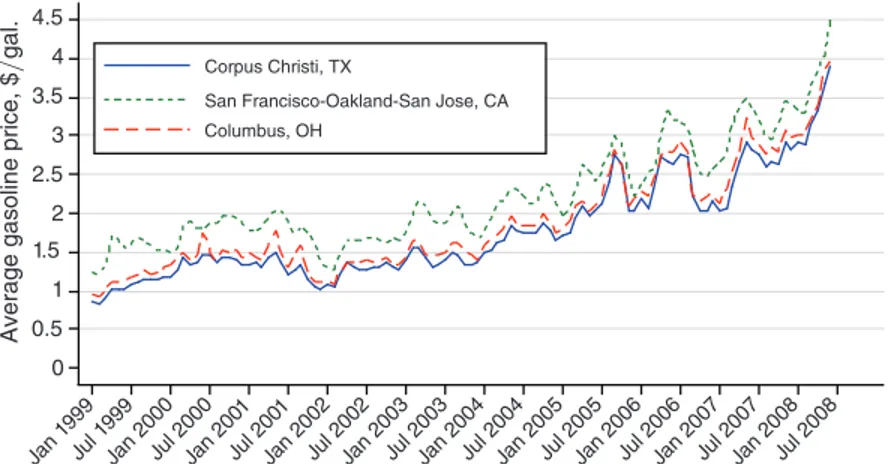
There is also substantial regional variation in gasoline prices. Figure 3 illus-trates this by comparing three DMAs: Corpus Christi, TX; Columbus, OH; and San Francisco-Oakland-San Jose, CA. California gasoline prices are substantially
higher than prices in Ohio (which are close to the median) and Texas (which are
low). While the three series generally track each other, in some months the series
are closer together, and in other months they are farther apart, reflecting the cross-sectional variation in the data.
5 In our data, the median Zip Code reports data from three stations on average over the months of the year. More
than 25 percent of Zip Codes have only one station reporting.
Figure 2. Monthly Average Gasoline Prices (National) 0 .5 1 1.5 2 2.5 3 3.5 4 4.5
Average gasoline price, $
/gal.
Jan 1 999
Jul 1 999
Jan 2000Jul 2000Jan 200 1 Jul 200
1
Figure 3. Monthly Average Gasoline Prices (by DMA)
Table 1—Summary Statistics (New cars)
Variable N Mean Median SD Min Max
GasolinePrice 1,863,403 2 1.8 0.67 0.82 4.6 MPG 1,863,403 22 22 5.7 10 65 Price 1,863,403 25,515 23,295 10,874 2,576 195,935 ModelYear 1,863,403 2004 2004 2.5 1997 2008 CarAge 1,863,403 0.79 1 0.46 0 3 TradeValue∗ 795,457 8,619 6,794 8,107 0 198,000 PctWhite 1,863,403 0.72 0.82 0.26 0 1 PctBlack 1,863,403 0.082 0.024 0.16 0 1 PctAsian 1,863,403 0.05 0.02 0.087 0 1 PctHispanic 1,863,403 0.12 0.053 0.18 0 1 PctLessHighSchool 1,863,403 0.15 0.12 0.13 0 1 PctCollege 1,863,403 0.38 0.36 0.19 0 1 PctManagement 1,863,403 0.16 0.15 0.082 0 1 PctProfessional 1,863,403 0.22 0.22 0.097 0 1 PctHeath 1,863,403 0.016 0.012 0.018 0 1 PctProtective 1,863,403 0.02 0.016 0.021 0 1 PctFood 1,863,403 0.041 0.035 0.031 0 1 PctMaintenance 1,863,403 0.028 0.021 0.029 0 1 PctHousework 1,863,403 0.027 0.024 0.021 0 1 PctSales 1,863,403 0.12 0.12 0.046 0 1 PctAdmin 1,863,403 0.15 0.15 0.054 0 1 PctConstruction 1,863,403 0.049 0.042 0.039 0 1 PctRepair 1,863,403 0.036 0.033 0.027 0 1 PctProduction 1,863,403 0.063 0.049 0.053 0 1 PctTransportation 1,863,403 0.05 0.044 0.037 0 1 Income 1,863,403 58,110 53,188 26,274 0 200,001 MedianHHSize 1,863,403 2.7 2.7 0.52 0 9 MedianHouseValue 1,863,403 178,306 144,700 131,956 0 1,000,001 VehPerHousehold 1,863,403 1.8 1.9 0.39 0 7 PctOwned 1,863,403 0.72 0.8 0.23 0 1 PctVacant 1,863,403 0.063 0.042 0.078 0 1 TravelTime 1,863,403 27 27 6.8 0 200 PctUnemployed 1,863,403 0.047 0.037 0.043 0 1 PctBadEnglish 1,863,403 0.044 0.016 0.078 0 1 PctPoverty 1,863,403 0.084 0.057 0.085 0 1 Weekend 1,863,403 0.25 0 0.44 0 1 EndOfMonth 1,863,403 0.25 0 0.43 0 1 EndOfYear 1,863,403 0.022 0 0.15 0 1
* This row summarizes the trade value for the subset of transactions that use trade-ins.
0 0.5 1 1.5 2 2.5 3 3.5 4 4.5
Average gasoline price, $
/ gal. Jan 1 999 Jul 1 999
Jan 2000Jul 2000Jan 200 1 Jul 200
1
Jan 2002Jul 2002Jan 2003Jul 2003Jan 2004Jul 2004Jan 2005Jul 2005Jan 2006Jul 2006Jan 2007Jul 2007Jan 2008Jul 2008
Corpus Christi, TX Columbus, OH
To create our final dataset, we draw a 10 percent random sample of all
transac-tions.6 After combining the three datasets this leaves us with a new car dataset of
1,863,403 observations and a used car dataset of 1,096,874 observations. Tables 1 and 2 present summary statistics for the two datasets.
III. Estimation and Results
In this section we estimate the short-run equilibrium effects of changes in gaso-line prices on the transaction prices, market shares, and unit sales of cars of different fuel economics. We separate our analysis by new and used markets. We will use
6 The 10 percent sample is necessary to allow for estimation of specifications with multiple sets of
high-dimensional fixed effects, including fixed effect interactions, that we use later in the article. Table 2—Summary Statistics (Used cars)
Variable N Mean Median SD Min Max
GasolinePrice 1,096,874 2 1.8 0.69 0.82 4.6 MPG 1,096,874 22 22 4.7 9.8 65 Price 1,096,874 15,637 14,495 8,281 1 173,000 ModelYear 1,096,874 2001 2001 3.5 1985 2008 CarAge 1,096,874 3.9 4 2.4 0 24 TradeValue∗ 435,813 5,233 3,000 5,992 0 150,000 PctWhite 1,096,874 0.7 0.81 0.28 0 1 PctBlack 1,096,874 0.11 0.028 0.2 0 1 PctAsian 1,096,874 0.038 0.013 0.07 0 1 PctHispanic 1,096,874 0.13 0.05 0.19 0 1 PctLessHighSchool 1,096,874 0.18 0.14 0.13 0 1 PctCollege 1,096,874 0.33 0.29 0.18 0 1 PctManagement 1,096,874 0.14 0.13 0.074 0 1 PctProfessional 1,096,874 0.2 0.19 0.092 0 1 PctHeath 1,096,874 0.019 0.014 0.02 0 1 PctProtective 1,096,874 0.021 0.017 0.021 0 1 PctFood 1,096,874 0.046 0.04 0.033 0 1 PctMaintenance 1,096,874 0.032 0.025 0.031 0 1 PctHousework 1,096,874 0.028 0.025 0.022 0 1 PctSales 1,096,874 0.12 0.11 0.044 0 1 PctAdmin 1,096,874 0.16 0.16 0.054 0 1 PctConstruction 1,096,874 0.056 0.049 0.041 0 1 PctRepair 1,096,874 0.04 0.037 0.027 0 1 PctProduction 1,096,874 0.075 0.061 0.059 0 1 PctTransportation 1,096,874 0.059 0.053 0.039 0 1 Income 1,096,874 50,684 46,556 22,031 0 200,001 MedianHHSize 1,096,874 2.7 2.7 0.51 0 8.5 MedianHouseValue 1,096,874 145,545 121,997 102,923 0 1,000,001 VehPerHousehold 1,096,874 1.8 1.8 0.39 0 7 PctOwned 1,096,874 0.69 0.76 0.24 0 1 PctVacant 1,096,874 0.067 0.048 0.076 0 1 TravelTime 1,096,874 27 26 6.9 0 200 PctUnemployed 1,096,874 0.053 0.041 0.046 0 1 PctBadEnglish 1,096,874 0.045 0.014 0.079 0 1 PctPoverty 1,096,874 0.1 0.072 0.095 0 1 Weekend 1,096,874 0.25 0 0.44 0 1 EndOfMonth 1,096,874 0.21 0 0.41 0 1 EndOfYear 1,096,874 0.017 0 0.13 0 1
the results estimated in this section to investigate, in Section IV, whether car buyers “undervalue” future fuel costs.
A. Specification and Variables for Car Price Results
At the most basic level, our approach is to model the effect of covariates on
short-run equilibrium price and (in a later subsection) quantity outcomes. For the car
industry, the short-run horizon is several months to a few years. During this time frame, a manufacturer can alter both price and production quantities, but its offering of models is predetermined, its model-specific capacity is largely fixed, and a
num-ber of input arrangements are fixed (labor contracts, in particular). While some of
these aspects become more flexible over a year or two (models can be tweaked,
some capacity can be altered), only over a long-run horizon (four years or more) can
a manufacturer introduce fundamentally different models into its product offering. We use a reduced form approach. In generic terms, this means regressing observed
car prices (P ) on demand covariates ( X D) and supply covariates ( X S):
(1) P = α 0 + α 1 X D + α 2 X S + ν.
The estimated α s we obtain from this specification will estimate neither parameters
of the demand curve nor those of the supply curve, but instead estimate the effect of each covariate on the equilibrium P, once demand and supply responses are both taken into account.
Our demand covariates are gasoline prices (the chief variable of interest), customer
demographics, and variables describing the timing of the purchase, all described in greater detail below. We also include region-specific year fixed effects, region-spe-cific month-of-year fixed effects, and detailed “car type” fixed effects. Supply
covari-ates should presumably reflect costs of production of new cars (raw materials, labor,
energy, etc.). We suspect that these vary little within the region-specific year and
region-specific month-of-year fixed effects that are already included in the specifica-tion. Furthermore, our interactions with executives responsible for short- to medium-run manufacturing and pricing decisions for automobiles indicate that, in practice, these decisions are not made on the basis of small changes to manufacturing costs.
We can write the specification we estimate more precisely as
(2) Pirjt = λ 0 + λ 1(GasolinePric e it · MPG Quartil e j ) + λ 2 Demo g it
+ λ 3 PurchaseTiming jt + δ j + τ r t + μ r t + ϵ ijt.
The price variable recorded in our dataset is the pre–sales tax price that the cus-tomer pays for the vehicle, including factory-installed accessories and options, and including any dealer-installed accessories contracted for at the time of sale that
con-tribute to the resale value of the car.7
7 Dealer-installed accessories that contribute to the resale value include items such as upgraded tires or a sound
We make two adjustments in order to make Pirjt capture the customer’s total wealth outlay for the car. First, we subtract off the manufacturer-supplied cash rebate to the customer if the car is purchased under a such a rebate, since the manufacturer pays that amount on the customer’s behalf. Second, we subtract from the purchase price any profit or add to the purchase price any loss the customer made on his or her trade-in. Dealers are willing to trade off profits made on the new vehicle transaction and profits made on the trade-in transaction, including being willing to lose money
on the trade-in.8 If a customer loses money on the trade-in transaction, part of his or
her payment for the new vehicle is an in-kind payment with the trade-in vehicle. By
adding such a loss to the negotiated (contract) price we adjust the price to include
the value of this in-kind payment. In equation (2), P irjt is the above-defined price for
transaction i in region r on date t for car j.
We estimate how gasoline prices affect the transaction prices paid for cars of different fuel economies. One might think that higher gasoline prices, by making car ownership more expensive, should lead to lower negotiated prices for all cars. Note, however, that cars do not increase uniformly in fuel cost: a compact car has lower fuel costs than an SUV at every gasoline price, but as gasoline price rises, its fuel cost advantage relative to the SUV actually rises. If enough people continue to want to own cars, even when gasoline prices increase, then higher gasoline prices may lead to increased demand for high fuel economy cars and decreased demand for low fuel economy cars, and consequently to the transaction price rising for the highest fuel economy cars and falling for the lowest fuel economy cars. To capture this, we estimate separate coefficients for the GasolinePrice variable depending on the fuel economy quartile into which car j falls. Specifically, we classify all
transac-tions in our sample by the fuel economy quartile (based on the EPA Combined Fuel
Economy MPG rating for each model) into which the purchased car type falls.9
Quartiles are redefined each year based on the distribution of all models offered (as
opposed to the distributions of vehicles sold) in that year. Table A1 in the online
Appendix reports the quartile cutoffs and mean MPG within quartile for all years of the sample.
We use an extensive set of controls. First, we control for a wide range of
demo-graphic variables (Demo g it) using data from the 2000 census: income, house value
and ownership, household size, vehicles per household, education, occupation,
aver-age travel time to work, English proficiency, and race of buyers.10 We use data at
the level of “block groups,” which, on average, contain about 1,100 people. We also
control for a series of variables that describe purchase timing (PurchaseTimingjt):
EndOf Year is a dummy variable that equals 1 if the car was sold within the last five days of the year; EndOf Month is a dummy variable that equals 1 if the car was sold within the last five days of the month; WeekEnd is a dummy variable that specifies whether the car was purchased on a Saturday or Sunday. If there are volume tar-gets or sales on weekends or near the end of the month or the year, we will absorb
their effects with these variables. For new cars, PurchaseTimingjt includes fixed
8 See Busse and Silva-Risso (2010) for further discussion of the correlation between dealers’ profit margins on
new cars versus trade-ins.
9 We obtain similar results if we estimate four separate regressions, thereby relaxing the constraint that the
parameters associated with the other covariates are equal across fuel economy quartiles.
effects for the difference between the model year of the car and the year in which the transaction occurs. This distinguishes between whether a car of the 2000 model year, for example, was sold in calendar 2000 or in calendar 2001. For used cars,
PurchaseTiming jt includes a flexible function of the car’s odometer, described in
more detail below, which controls for depreciation over time.
We include year, τ rt , and month-of-year, μ rt, fixed effects corresponding to when
the purchase was made. Both year and month-of-year fixed effects are allowed to
vary by the geographic region (34 throughout the United States) in which the car
was sold.11 The identifying variation we use is therefore variation within a year
and region that differs from the average pattern of seasonal variation within that region. To examine the robustness of our results to which components of variation in the data are used to identify the effect of gasoline prices, we repeat our estimation with a series of different fixed effect specifications in Section VA. We also control for detailed characteristics of the vehicle purchased by including “car type” fixed
effects ( δ j ). A “car type” in our sample is the interaction of make, model, model
year, trim level, doors, body type, displacement, cylinders, and transmission. (For
example, one “car type” in our data is a 2003 Honda Accord EX four-door sedan
with a four-cylinder 2.4-liter engine and automatic transmission).
The coefficients of primary interest will be the coefficients on the monthly, DMA-level gasoline price measure. This variable contains both cross-sectional and inter-temporal variation. Cross-sectional variation arises from factors such as differences
across locations in transportation costs (or transportation capacity), variation in the
degree of market power, and differences in the costs of required gasoline formula-tions. Intertemporal variation in gasoline prices arises mostly from differences in the world price of oil. Because we use year and month-of-year fixed effects, both interacted with region, the component of the intertemporal variation that identifies our results will be within-year variation in gasoline prices that differs from the typi-cal seasonal pattern of variation for the region. The component of cross-sectional variation that will identify our results will be persistent differences among DMAs within a region in factors such as transportation costs or market power, as well as month-to-month fluctuations in the gasoline price differentials between DMAs or month-to-month fluctuations in the gasoline price differentials between regions that
differs from the typical seasonal pattern.12 By using a variable that contains both
cross-sectional and intertemporal variation, our specification assumes that car buy-ers respond equally to both components of variation. In other words, we assume that intertemporal variation arising from changes in world oil prices and fluctuations in local market conditions both matter to car buyers in determining their forecasts of future gasoline prices, and in driving their decisions about what vehicles to buy. (In Section VC we consider specifications that use more geographically aggregated measures of gasoline price, one a national price series and another that varies by five regions of the country defined by Petroleum Administration for Defense Districts
11 See Table A13 in the online Appendix for a list of regions and the DMAs within each region.
12 The average price of gasoline in a DMA-month (our unit of observation) is $1.91; the standard
devia-tion is 0.68. The “within region-year” standard deviadevia-tion is 0.21, a value that is 11 percent of the mean. The “between region-year” standard deviation is 0.72. (The “within” standard deviation is the standard deviation of
XDMA, month − _X region, year + X _ where _X region, year is the average for the region-year and _X is the global mean. The between standard deviation is the standard deviation of _X region, year).
(PADDs)). A second, less obvious assumption implied by this specification is that vehicles are not traded across regions in response to gasoline price differentials.
Before describing the results, we note that our estimates should be interpreted as estimates of the short-run effects of gasoline prices, meaning effects on prices, market shares, or sales over the time horizon in which manufacturers would be unable to change the configurations of cars they offer in response to gasoline price changes, a period of several months to a few years. Persistently higher gasoline prices would presumably cause manufacturers to change the kinds of vehicles they choose to produce, as US manufacturers did in the 1970s at the time of the first oil
price shock.13 The nature of our data, their time span, and our empirical approach
are all unsuited to estimating what the long-run effects of gasoline price would be on prices or sales. The short-run estimates are nevertheless useful, we believe, for two reasons. First, the short run effect is indeed the effect we want to estimate in order to investigate the question of consumer myopia. More generally, short-run
effects are important for auto manufacturers in the short-to-medium term
(espe-cially if financial solvency is an issue) and because they yield some insight into the
size of the pressures to which manufacturers are responding as they move toward the long run.
B. New Car Price Results
We first estimate equation (2) using data on new car transactions. The full results
from estimating this specification are presented in Table A2 of the online Appendix. The variable of primary interest is GasolinePrice in month t in the DMA in which
customer i resides.14 This variable is interacted with an indicator variable which
equals 1 if the observation is for cars in MPG quartile k. The coefficients of interest
are the four coefficients in the vector λ 1 which represent the effect of gasoline prices
on the prices of cars in each of the four MPG quartiles; these coefficients and their standard errors are reported in Table 3. To account for correlation in the errors due to either supply or demand factors, we cluster the standard errors at the DMA level.
These estimates indicate that a $1 increase in the price of gasoline is associated
with a lower negotiated price of cars in the lowest fuel economy quartile (by $250)
13 As gasoline prices began to fall in the early 1980s, CAFE standards also affected manufacturer offerings. 14 Another approach would be to use a variable that represents gasoline price expectations, perhaps based on
futures prices for crude oil. In Section VB we explore such an approach.
Table 3—Gasoline Price Coefficients from New Car Price Specification
Variable Coefficient SE
GasolinePrice × MPG Quart 1 (lowest fuel economy) −250*** (72)
GasolinePrice × MPG Quart 2 −96*** (37)
GasolinePrice × MPG Quart 3 −11 (26)
GasolinePrice × MPG Quart 4 (highest fuel economy) 104** (47)
*** Significant at the 1 percent level.
** Significant at the 5 percent level.
but a higher price of cars in the highest fuel economy quartile (by $104), a relative price difference of $354. Overall, the change in negotiated prices appears to be monotonically related to fuel economy. Note that this is an equilibrium price effect; it is the net effect of the manufacturer price response, any change in consumers’ willingness-to-pay, and the change in the dealers’ reservation price for the car.
C. Used Car Price Results
In this section, we estimate the effect of gasoline prices on the transaction prices
of used cars by estimating equation (2) (with some modifications) using the data
on used car transactions. We observe all the same car characteristics for used cars that we do for new cars, enabling us to use all the covariates to estimate the used car price results that we used to estimate the results for new cars, including
identi-cal “car type” fixed effects.15 However, there is one important difference between
used cars and new cars. A new car of a given model-year can sell only during that model-year; a used car of a given model-year can sell in many different years. Over that time period, tastes may change, and individual vehicles will depreciate. To capture the effect of depreciation on used car transaction prices, we include a
spline in odometer (Odom) when we estimate equation (2) using the data on used
car transactions.16 The spline has knots at 10,000-mile increments, allowing a
dif-ferent per mile rate of depreciation for each 10,000-mile range of mileage.17 We
interact the spline with segment indicator variables to allow different types of cars to have different depreciation paths, and with indicators for five regions of the
country defined by Petroleum Administration for Defense Districts (PADDs) to
allow these paths to vary regionally.18 In addition, in order to allow for changes in
tastes for different vehicle segments over time, we replace the year fixed effects in
equation (2) with segment-specific year fixed effects.19 In the new car specification
(equation (2)) we allowed the year fixed effects to differ by region. We also allow the segment-specific year fixed effects to vary by geography; however, to reduce the number of fixed effects we have to estimate, we now interact the
segment-specific year fixed effects with PADD instead of region.20 This three way
interac-tion controls for business cycle fluctuainterac-tions that affect the entire car market, for
year-to-year changes in tastes for different segments of cars (such as the increasing
popularity of SUVs), and allows both of these effects to vary across the five PADD
15 The definition of the price of the car is also the same. We subtract any profits (or add any losses) the customer
makes trading in a car he or she currently owns in exchange for a different car. Used cars do not have any manu-facturer rebate to subtract.
16 In using odometer, our approach resembles Sallee, West, and Fan (2009). We differ from Allcott and Wozny
(2011), who use car age to measure depreciation. We use odometer for two reasons. First we find that adding car age does very little (in an R 2 sense) to explain depreciation once odometer is accounted for. Second, since odometer
varies across individual vehicles, and does not move in lockstep with calendar time, odometer is less collinear with gasoline price than car age is. Using odometer thus increases our ability to identify a gasoline price effect in the data, if there is one.
17 We drop the 0.97 percent of the sample with odometer readings of 150,000 miles or greater.
18 There are seven segments: Compact, Midsize, Luxury, Sporty, SUV, Pickup, and Van. The five PADDs are
East Coast, Midwest, Gulf Coast, Rockies, and West Coast.
19 In the new car specification, changes in tastes are captured by the car type fixed effects since any particular car
type sells as a new car only for one model-year.
regions of the country. Taking into account these modifications, the specification we estimate for used cars is
(3) Pirjt = λ 0 + λ 1(GasolinePric e it · MPG Quartil e j )
+ f 10, 000(Odo m i, λ 2rj ) · Segmen t j · PAD D r
+ λ 3 Demo git + λ 4 PurchaseTiming jt + δ j + τ rjt + μ rt + ϵ ijt ,
where τ rjt is the year-segment-PADD fixed effect.
One could also consider allowing depreciation to vary by MPG quartile and
region instead of by segment and region. (In other words, one could replace
f10, 000(Odo m i, λ 2rj ) · Segmen t j · PAD D r in equation (3) with f 10, 000(Odo m i, λ 2rj )
· MPG Quartil e j · PAD D r .) A priori, we think that segment is a better
categoriza-tion for vehicle depreciacategoriza-tion than MPG quartile. Our belief is that SUVs are more likely to depreciate according to the same pattern as other SUVs, and luxury cars more like other luxury cars, than a midsize SUV and a high horsepower luxury car are to depreciate according to the same pattern just because they fall in the same MPG quartile. Additionally, allowing depreciation to vary by MPG quartile instead of segment divides vehicles into the same categorization for measuring gasoline price effects as for measuring depreciation effects. This will substantially increase the ability of our odometer measure to soak up any correlated gasoline price effect and will make it difficult for us to identify whatever gasoline price effect is in the data. Nevertheless, we report results below that use this alternative interaction.
As we did for new cars, we estimate the effect of gasoline prices on used car prices separately by the MPG quartile of the used car being purchased. The full
results are reported in column 1 of Table A3 in the online Appendix. (Column 2 of
Table A3 in the online Appendix reports the results if depreciation is allowed to vary
by MPG quartile instead of segment.) The gasoline price coefficients from columns
1 and 2 of Table A3 are reported in panels 1 and 2 of Table 4.
These estimates show a much larger effect on the equilibrium prices of used cars than was estimated for new cars. The estimates in column 1 indicate that a $1 increase in gasoline price is associated with a lower negotiated price of cars in the
lowest fuel economy quartile (by $1,182) but a higher price of cars in the highest
Table 4—Gasoline Price Coefficients from Used Car Price Specification
Variable Coefficient SE Coefficient SE
GasolinePrice × MPG Quart 1 (lowest fuel economy) −1,182*** (42) −783*** (49)
GasolinePrice × MPG Quart 2 −101 (62) 118** (54)
GasolinePrice × MPG Quart 3 468*** (36) 369*** (33)
GasolinePrice × MPG Quart 4 (highest fuel economy) 763*** (44) 360*** (36) Depreciation varies by Segment × PADD MPG Quartile × PADD
*** Significant at the 1 percent level.
** Significant at the 5 percent level.
fuel economy quartile (by $763), a relative price difference of $1,945, compared to
a difference of $354 for new cars.21
D. Specification and Variables for Car Quantity Results
In this section we estimate the reduced form effect of gasoline prices on the equi-librium market shares and sales of new cars of different fuel economies. We can write
an analog of equation (1) that gives a reduced form expression for new car quantity,
or some function of quantity, as a function of demand and supply covariates:
(4) Q = β 0 + β 1 X D + β 2 X S + η.
As with equation (1), the estimated β s will measure neither parameters of the
demand curve, nor parameters of the supply curve, but instead the estimated short-run effects of the covariates on equilibrium quantities.
We will estimate two variants of equation (4). In the first variant, we will use the
market shares of vehicles of different types as an outcome variable, rather than unit sales. There are two advantages to this approach. First, using market share con-trols for the substantial fluctuation in aggregate car sales over the year. Second, this approach enables us to control for transaction- and buyer-specific effects on car purchases. The disadvantage is that if changes in gasoline prices affect total unit sales of new cars too much, changes in market share may not correspond to changes
in unit sales. In light of this, we will also estimate a second variant of equation (4)
using two different measures of unit sales.
In our market share regression we estimate the effect of gasoline prices on market shares of cars of different fuel economies using a set of linear probability models that can be written as
(5) Ii r t( j ∈ K ) = γ 0 + γ 1 GasolinePric e it + γ 2 Demo git
+ γ 3 PurchaseTimingjt + τ r t + μ r t + ϵ ijt ;
Iir t( j ∈ K ) is an indicator that equals 1 if transaction i in region r on date t for car
type j was for a car in class K.22 We use quartiles of fuel economy to define the
classes into which a car type falls. As described in Section IIIA, quartiles are based
on the distribution of fuel economies of car models for sale in a given year (i.e., the
model-weighted, not sales-weighted, distribution).
21 The estimates in panel 2 of Table 4, which allows depreciation to vary by MPG quartile, imply that a $1 increase
in the price of gasoline would be predicted to increase the price of a car in the highest fuel economy quartile of cars relative to that in the lowest fuel economy by $1,143. Note that the results in panel 2 are nonmonotonic; they imply that an increase in the price of gasoline increases the price of an MPG quartile 3 used car by more than (statistically, by the same amount as) it increases the price of a quartile 4 car. Quartile 4 cars all have lower fuel costs per mile than quartile 3 cars, so one should be cautious about calculating implicit discount rates on the basis of this column.
22 Our results do not depend on the linear probability specification; we obtain nearly identical results with a
The variable of primary interest is GasolinePrice, which is specific to the month in which the vehicle was purchased and to the DMA of the buyer. We use the same demographic and purchase timing covariates and the same region-specific year and region-specific month-of-year fixed effects that we used to estimate the effect of
gas-oline prices on new car prices in equation (2), although in estimating equation (5)
we cannot use the “car type” fixed effects that we used to estimate equation (2)
because “car type” would perfectly predict the fuel economy quartile of the
transac-tion. We will estimate equation (5) four times, once for each fuel economy quartile.
In order to estimate the effect of gasoline prices on unit sales, we use two dif-ferent measures of unit sales. The first measure we use aggregates our individual
transaction data into unit sales by dealer, for each month, by MPG quartile.23 Using
this measure, we estimate
(6) Qdkrt = γ 0 + γ 1(GasolinePric e dt · MPG Quartil e k )
+ γ 2 MPG Quartil ek + δ d + τ rt + μ rt + ϵ dkrt ;
Qdkr t is the unit sales at dealer d located in region r for vehicles in MPG quartile k
that occur in month t. The variable of primary interest is the GasolinePrice in month
t in the DMA in which dealer d is located. The coefficients of primary interest are
γ 1 . These coefficients estimate the average effect of gasoline prices on new car sales
within a fuel economy quartile. We include fixed effects for each of the MPG
quar-tiles and for individual dealers ( δ d ). Finally, as in equation (5), we include year,
τ rt, and month-of-year, μ r t, fixed effects that are allowed to vary by the geographic
region of the dealer.
While this measure enables us to look at effects on unit sales (instead of market
share) while still controlling for many local characteristics (via dealer fixed effects),
the estimated coefficients will represent the effects on sales at an average dealer. In our final specification, we measure sales at the national level using information from
Ward’s Auto Infobank.24 Using these data, we estimate
(7) Qkt = γ 0 + γ 1(GasolinePric e t · MPG Quartil e k )
+ γ 2 MPG Quartil ek + τ t + μ t + ϵ kt;
Qkt is the national unit sales for vehicles in MPG quartile k that occur in month t.25
The variable of primary interest is again GasolinePrice, which is now measured as the national average in month t. The coefficients of interest are the four coefficients
in the vector γ 1 which represent the effects of gasoline prices on the sales of cars in
23 We aggregate from our full dataset, not the 10 percent random sample that we use elsewhere in the article. 24 Our transaction data are from a representative sample of dealers, according to our data source. So one approach
might be simply to use our data and multiply by the inverse of the sample percentage to get a national figure. Unfortunately, the sample percentage changes slightly over time, and we don’t know the year-to-year scaling factor.
25 Ward’s reports sales data for some cars by a more aggregate model designation than the EPA uses to report
MPGs. We use the sales fractions in our transaction data to allocate models to which this issue applies in the Ward’s data into MPG quartiles.
each of the four MPG quartiles. We include fixed effects for each of the MPG quar-tiles, and for year, τ t , and month-of-year, μ t.26
E. New Car Market Share Results
We first consider the effect of gasoline prices on the market shares of new cars in different quartiles of fuel economy. Quartiles are redefined each year based on the
distribution of all models offered (as opposed to the distributions of vehicles sold)
in that year.
In order to estimate equation (5), we define four different dependent variables. The
dependent variable in the first estimation is 1 if the purchased car is in fuel economy quartile 1, and 0 otherwise. The dependent variable in the second estimation is 1 if the purchased car is in fuel economy quartile 2, and 0 otherwise, and so on.
The full estimation results are reported in Table A4 in the online Appendix. The
estimated gasoline price coefficients ( γ 1 ) for each specification are presented in
Table 5. We also report the standard errors of the estimates, and the average market
share of each MPG quartile in the sample period. (Since the quartiles are based on
the distribution of available models, market shares need not be 25 percent for each
quartile.) Combining information in the first and third column, we report in the last
column the percentage change in market share that the estimated coefficient implies would result from a $1 increase in gasoline prices.
These results suggest that a $1 increase in gasoline price decreases the market share of cars in the lowest fuel economy quartile by 5.7 percentage points, or 27.1 percent. Conversely, we find that a $1 increase in gasoline price increases the market share of cars in the highest fuel economy quartile by 7.1 percentage points, or 21.1 percent. This provides evidence that higher gasoline prices are associated with the purchase of cars with higher fuel economy. Notice that these estimates do not simply reflect an over-all trend of increasing gasoline prices and increasing fuel economy; since we control for region-specific year fixed effects, all estimates rely on within-year, within-region variation in gasoline prices and car purchases. Nor are the results due to seasonal cor-relations between gasoline prices and the types of cars purchased at different times of year, since the regressions control for region-specific month-of-year fixed effects.
26 In results available from the authors, we use a third unit sales measure. That third measure uses the
informa-tion in our transacinforma-tion data about the regional distribuinforma-tion of sales within an MPG quartile to divide the Ward’s national sales into regional sales. Specifically, for each month in the sample, we calculate from the transaction data the fraction of sales in each MPG quartile that occurred in each region. We then designate that fraction of the Ward’s sales in the corresponding MPG quartile to have occurred in the corresponding region.
Table 5—Gasoline Price Coefficients from New Car Market Share Specification
Fuel economy Coefficient SE
Mean market share
Percent change in share MPG Quartile 1 (lowest fuel economy) −0.057*** (0.0048) 21.06 −27.1
MPG Quartile 2 −0.014*** (0.004) 20.95 −6.7
MPG Quartile 3 0.0002 (0.0027) 24.28 0.1
MPG Quartile 4 (highest fuel economy) 0.071*** (0.0058) 33.72 21.1
*** Significant at the 1 percent level.
** Significant at the 5 percent level.
F. New Car Sales Results
While the market share results allow us to investigate the effect of gasoline prices on automobile purchase choices while controlling for transaction- and buyer-spe-cific characteristics, they do not allow us to draw inferences directly about changes in unit sales. Changes in gasoline prices may be correlated, for macroeconomic reasons, with changes in the total number of vehicles sold. A higher market share of a smaller market could correspond to a unit decrease in sales, just as a smaller market share of a bigger market could correspond to a unit increase in sales. In this
subsection, we report the results of our two unit sales specifications, equation (6)
and equation (7).
The coefficient estimates for these two specifications are reported in Tables 6 and 7. The tables report the estimated gasoline price coefficients for each of the four MPG quartiles, the average unit sales, and the percentage change relative to the average implied by the coefficients for a $1 increase in the price of gasoline. On average, a dealer sells 11.2 cars per month in the lowest fuel economy quartile of available cars; a $1 increase in gasoline prices is estimated to reduce that number by 3.1 cars, or 27.7 percent. On average, dealers sell 17.8 cars per month in the highest fuel economy quartile of cars; a $1 increase in gasoline prices increases that number by 2.1 cars, or 11.8 percent. Adding up the predicted effects across quartiles shows that an increase in gasoline prices is predicted to reduce the total sales of new cars. Consistent with this, the percentage changes in unit sales are more negative quartile-by-quartile than the percentage changes in market share reported in the previous
section.27
27 This is consistent with Knittel and Sandler (2012) which finds that increases in gasoline prices reduce the
scrappage rates of used vehicles, in aggregate.
Table 6— Gasoline Price Coefficients from Dealer-Level Unit Sales Specification
Fuel economy Coefficient SE
Average cars sold per month in dealer
Percent change in sales MPG Quartile 1 (lowest fuel economy) −3.1*** (0.091) 11.2 −27.7
MPG Quartile 2 −0.83*** (0.087) 11.1 −7.5
MPG Quartile 3 −0.71*** (0.088) 13.0 −5.5
MPG Quartile 4 (highest fuel economy) 2.1*** (0.11) 17.8 11.8
*** Significant at the 1 percent level.
** Significant at the 5 percent level.
* Significant at the 10 percent level.
Table 7— Gasoline Price Coefficients from National Unit Sales Specification
Fuel economy Coefficient SE per month nationallyAverage cars sold Percent changein sales MPG Quartile 1(lowest fuel economy) −79,169*** (9,421) 291,533 −27.2
MPG Quartile 2 −14,761 (9,994) 262,453 −5.6
MPG Quartile 3 −30,029*** (9,609) 329,466 −9.1
MPG Quartile 4 (highest fuel economy) 40,116*** (11,800) 372,998 10.8
*** Significant at the 1 percent level.
** Significant at the 5 percent level.
According to the estimates using the Ward’s national sales data, reported in the next table, when gasoline prices increase by $1, there are 79,169 fewer cars per month sold in the lowest fuel economy quartile of cars. This is a 27.2 percent decrease relative to the 291,533 monthly average in this quartile. In the highest fuel economy quartile, a $1 increase in gasoline prices is associated with an increase in monthly sales of 40,116 cars, a 10.8 percent increase on the average monthly sales in this quartile of 372,998.
Overall, the results we obtain using unit sales tell a very consistent story whether they are measured at the dealer or national level. They are also broadly consistent with the market share results estimated in the previous section, with the primary difference being that the unit sales results reveal a reduction in total car purchases when gasoline prices increase that is masked in the market share results.
G. Used Car Transaction Share Results (an Aside)
While we can easily estimate equation (5) using our data on used car transactions,
the estimates do not have the same interpretation as the estimates for new cars. Changes in the market share of new cars measure how the incremental additions to the US vehicle fleet change when gasoline prices change. The analogous estimates arising from the used car data would not measure changes in market share in this sense, but instead changes in “transaction share”; namely, how gasoline price affects the share of used car transactions that are for cars in different quartiles. For com-pleteness, we present these results briefly.
We estimate equation (5) using data from used car transactions at the same
dealer-ships at which we observe new car transactions. The full results of transaction share effects of gasoline prices by MPG quartiles are reported in Table A5 in the online Appendix. The gasoline price coefficients are reported in Table 8.
The results are both smaller in magnitude and weaker in statistical significance than the analogous results for new cars.
Summary of Results.—Overall, we see a modest effect of gasoline prices on new car transaction prices. The predicted effect of a $1 gasoline price increase is to increase the price difference between the highest and lowest fuel economy quartiles of new cars by $354. The estimated effects are much larger for used cars; in this market, the predicted effect is to increase the price difference between the highest and lowest fuel economy quartiles by $1,945.
We find both statistically and economically significant effects of gasoline prices on new car sales, measured either as market shares or as unit sales. This is particularly
Table 8—Gasoline Price Coefficients from Used Car Transaction Share Specification
Fuel economy Coefficient SE Mean share
Percent change in share MPG Quartile 1 (lowest fuel economy) 0.00018 (0.0069) 24.19 0.07
MPG Quartile 2 −0.0077 (0.006) 20.89 −3.7
MPG Quartile 3 0.017 (0.011) 27.32 6.2
true for the highest fuel economy and lowest fuel economy quartiles, where market share shifts by more than 20 percent in response to a $1 increase in gasoline prices, and where unit sales decrease by more than 25 percent for the lowest fuel economy quartile and rise by more than 10 percent for the highest fuel economy quartile.
IV. Consumer Valuation of Future Fuel Costs
In this section, we draw upon the estimates in the previous section to investigate whether consumers exhibit “myopia” about future fuel costs of different cars when they are considering the up-front purchase decision. We will begin by describing our empirical approach.
A. Empirical Approach
The basic starting point for the consumer myopia literature is a simple idea: an increase in the expected future usage cost of a durable good should not change consumers’ total willingness-to-pay for the good, all else equal. This means that if the usage cost component of the total cost rises, the up-front cost must fall by an
equal amount if consumers (whose total willingness-to-pay is unchanged) are to
keep purchasing the good. A direct approach to testing whether consumers “cor-rectly” value future fuel costs would be to estimate a demand relationship in which expected future fuel costs were included as a covariate, and test whether the relevant coefficient has the value that would be implied by consumers correctly valuing fuel costs.
In the automotive setting, there are two difficulties to actually estimating this rela-tionship. One is that, in the cross-section, differences between cars in fuel costs are often related to differences between those cars in other attributes that are valued by consumers as goods; for example, size, weight, power, or other, unobservable attri-butes. This can make the empirical cross-sectional relationship between price and fuel cost positive. Of course, adequate controls for characteristics, or detailed car
fixed effects, could remedy this.28
A second problem is that if intertemporal variation in gasoline prices is used to identify the relationship between a car’s price and its future fuel cost, the “all else equal” condition is violated: a rise in the price of gasoline which increases the cost of operating one car will increase the cost of operating all gasoline-powered cars. This means that if consumers are sufficiently unwilling to substitute away from cars as a whole, a rise in the price of gasoline might well increase the price of cars with relatively high fuel economy even if their operating costs have actually gone up, because the operating cost would have decreased relative to that of a low fuel economy car.
To see how this latter point affects the estimation of the relationship between future fuel costs and car prices, consider a market with two vehicles, 1 and 2.
Suppose that the price of vehicle i is given by pi and that the present discounted
28 A recent example of a paper that takes this approach is Espey and Nair (2005), who estimate a hedonic
regres-sion of list prices on a variety of attributes for a cross-sectional sample of 2001 model year cars. They conclude that consumers use fairly low discount rates when valuing future fuel cost savings.
value of the expected future gasoline cost for operating vehicle i over its lifetime is
given by Gi. For simplicity, suppose that demand is linear, implying the demand for
vehicle 1 can be written as
(8) q1 = α 1 + β 11( p 1 + G 1 ) + β 12( p 2 + G 2 ).
Solving this for price implies the following relationship:
(9) p1 = − γ G 1 + 1 _ β 11 q1 − α _ 1 β 11 − β _ 12 β 11 ( p 2 + G 2 ),
where γ = −1 is implied by consumers who correctly value future fuel costs. One
could test whether consumers really do behave this way by estimating γ as a free
parameter.
There are three difficulties in estimating this relationship in practice. First, a gen-eral model would have to specify the price of vehicle i as a function of the fuel cost of vehicle i and of the fuel costs of all other vehicles separately. Given the large
number of vehicles offered in the US market, this would be difficult to implement.29
A second difficulty is that there may be endogeneity between qi and pi, arising from
a supply relationship between the two variables.
In this article, we will take an alternative approach. Our approach is to combine our reduced-form estimates of price and quantity effects with estimates of the elas-ticity of demand for new cars, and estimates of future gasoline prices, vehicle miles traveled, and vehicle survival rates in order to address the question of whether con-sumers are myopic with respect to future fuel costs. Note that these assumptions are very similar to the set of assumptions that must be made in the structural approach. In this sense, the two approaches do not differ in how many assumptions must be imposed, but at what stage in the analysis they are imposed. The structural approach imposes them earlier and is able thereby to estimate a single parameter that captures the degree of consumer myopia and can be used in counterfactual simulations. The reduced form approach will be more amenable to examining the effect of a variety of assumptions about vehicle miles traveled, future gasoline prices, and vehicle sur-vival rates. We will present a range of estimates; it will be fairly straightforward for readers to substitute their own assumptions as well.
B. Consumer Myopia Results
In this section we address the question of whether consumers are myopic about future gasoline prices when they make car purchase decisions. Analyzing this means, in simple terms, comparing the effects of gasoline price changes on buyers’ will-ingness-to-pay for cars of different fuel economies to the changes in the discounted
29 An alternative approach, used by Allcott and Wozny (2011), is to specify a nested logit demand system and
then to solve for equilibrium prices. The benefit of this approach is that in the logit model the usage cost of all other vehicles drops out of the estimating equation once the market share of each car is divided by the share of the outside good. The cost is that it imposes a specific functional form assumption on the data. If the model is not a good match for the data, the estimates could lead to erroneous inferences.