Decision models to prioritize maintenance and renewal alternatives

Publisher’s version / Version de l'éditeur:

Vous avez des questions? Nous pouvons vous aider. Pour communiquer directement avec un auteur, consultez la première page de la revue dans laquelle son article a été publié afin de trouver ses coordonnées. Si vous n’arrivez pas à les repérer, communiquez avec nous à PublicationsArchive-ArchivesPublications@nrc-cnrc.gc.ca.

Questions? Contact the NRC Publications Archive team at

PublicationsArchive-ArchivesPublications@nrc-cnrc.gc.ca. If you wish to email the authors directly, please see the first page of the publication for their contact information.

https://publications-cnrc.canada.ca/fra/droits

L’accès à ce site Web et l’utilisation de son contenu sont assujettis aux conditions présentées dans le site LISEZ CES CONDITIONS ATTENTIVEMENT AVANT D’UTILISER CE SITE WEB.

Joint International Conference on Computing and Decision Making in Civil and Building Engineering [Proceedings], pp. 2594-2603, 2006-06-14

READ THESE TERMS AND CONDITIONS CAREFULLY BEFORE USING THIS WEBSITE. https://nrc-publications.canada.ca/eng/copyright

NRC Publications Archive Record / Notice des Archives des publications du CNRC :

https://nrc-publications.canada.ca/eng/view/object/?id=08a91d93-380c-4727-b9fc-525013924379 https://publications-cnrc.canada.ca/fra/voir/objet/?id=08a91d93-380c-4727-b9fc-525013924379

NRC Publications Archive

Archives des publications du CNRC

This publication could be one of several versions: author’s original, accepted manuscript or the publisher’s version. / La version de cette publication peut être l’une des suivantes : la version prépublication de l’auteur, la version acceptée du manuscrit ou la version de l’éditeur.

Access and use of this website and the material on it are subject to the Terms and Conditions set forth at Decision models to prioritize maintenance and renewal alternatives Vanier, D. J.; Tesfamariam, S.; Sadiq, R.; Lounis, Z.

http://irc.nrc-cnrc.gc.ca

Decision models to prioritize maintenance and renewal

alternatives

N R C C - 4 5 5 7 1

V a n i e r , D . ; T e s f a m a r i a m , S . ;

S a d i q , R . ; L o u n i s , Z .

A version of this document is published in / Une version de ce document se trouve dans: Joint International Conference on

Computing and Decision Making in Civil and Building Engineering, Montréal, QC., June 14-16, 2006, pp. 2594-2603

DECISION MODELS TO PRIORITIZE

MAINTENANCE AND RENEWAL ALTERNATIVES

Dana Vanier 1, Solomon Tesfamariam 2, Rehan Sadiq 3 and Zoubir Lounis 4

ABSTRACT

Publicly owned infrastructure forms a large portion of the existing infrastructure in Canada and elsewhere. Typically, asset managers must make decisions about maintenance and renewal alternatives based on sparse data about the current state of their infrastructure assets, the relative risk of failure of these assets, and the life cycle costs of proposed interventions. The infrastructure in any one organization can consist of a diverse set of assets ranging from bridges to buildings and from buried to overhead utilities. The optimal selection of proposed interventions across this broad spectrum of assets is also problematic, and currently it is performed in a subjective manner. This paper identifies a number of prioritization techniques that can be used to compare and rank repair and renewal projects. This research does not attempt to develop models to select the “correct projects” or even to identify the best decision model or prioritization technique; rather, it attempts to illustrate by example the results of specific decision-making paradigms.

KEY WORDS

infrastructure, asset management, decision support systems (DSS), multi-criteria decision-making (MCDM), multi-objective optimization (MOO), analytic hierarchy process (AHP), fuzzy synthetic evaluation (FSE).

INTRODUCTION

Publicly owned infrastructure forms a large portion of the existing infrastructure in Canada and elsewhere. The value of infrastructure assets owned by Canadian governments (federal, provincial, regional, municipal) or para governmental agencies (universities, colleges, school boards, hospitals, etc.) is estimated in the trillions of dollars (Vanier and Rahman 2004) and the recommended annual level of investment for both maintenance and renewal (M & R) is in the range of 4-6% of the asset replacement value (Vanier and Rahman 2004). However, the current M & R spending is considerably less than the amount required to keep our publicly owned infrastructure in an acceptable condition (ASCE 2005). As a result, this

1

Institute for Research in Construction, NRC, 1200 Montreal Road, Ottawa, Canada, Phone 613/993-9699, FAX 613/954-5984, dana.vanier@nrc-cnrc.gc.ca

2

Institute for Research in Construction, NRC, 1200 Montreal Road, Ottawa, Canada, Phone 613/993-2448, FAX 613/954-5984, solomon.tesfamariam@nrc-cnrc.gc.ca

3

Institute for Research in Construction, NRC, 1200 Montreal Road, Ottawa, Canada, Phone 613/993-6282, FAX 613/954-5984, rehan.sadiq@nrc-cnrc.gc.ca

4

Institute for Research in Construction, NRC, 1200 Montreal Road, Ottawa, Canada, Phone 613/993-5412, FAX 613/952-8102, zoubir.lounis@nrc-cnrc.gc.ca

“infrastructure gap” between the available funding and the required M & R funds is growing. These problems, compounded by continuing infrastructure deterioration, have reached a point of concern for many owners and managers of these assets (TRM 2003).

Typically, asset managers must make decisions about M & R alternatives based on sparse data about the ‘current state’ of their infrastructure assets, the ‘relative risk of failure’ of these assets (and their individual components), the “initial costs”, and ‘life cycle costs’ of proposed interventions. As sufficient funds do not exist to maintain or renew all deficient assets in any one jurisdiction, it is necessary to prioritize and select those interventions that come closest to meeting the organization’s prime objectives. Although it is possible to select the optimal M & R investment in a current year, it is very difficult to optimize the selection of M & R investments each year in a short or a long planning horizon (e.g. 5 or 10 years)

The infrastructure in any one organization consists of a diverse set of assets ranging from bridges to buildings and from buried to overhead utilities. As a result, it is difficult to compare the benefits and costs of repairing or renewing these dissimilar types of assets. Infrastructure in such diverse asset portfolios, such as those managed by municipalities, is also in a constant state of flux: priorities shift, assets deteriorate, technologies evolve, portfolio size increases/decreases, etc. In addition, the performance indicators used to evaluate the individual systems can be very subjective or virtually non-existent. On top of all this, decision-makers at higher levels (both technical and political) must optimize their investments based on a number of uncertain, and at times subjective and conflicting, criteria, including: type of maintenance intervention, overall network performance, risk and reliability, life cycle costs, desired levels of service, budgetary constraints, construction costs, social costs, etc.

The optimal selection of intervention projects across a broad spectrum of assets is therefore problematic, and is currently performed in practice in a subjective manner or using minimal decision support tools (NAMSG 2004). Different prioritization techniques can be selected and used, as can different ranking and rating systems. However, as illustrated in the following examples, the prioritization results can be conflicting and confusing.

FRAMEWORK FOR DECISION SUPPORT SYSTEM (DSS)

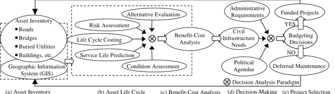
Figure 1 illustrates a proposed framework for a decision support system (DSS) for infrastructure management (Vanier and Lounis 2006).

Life Cycle Costing

Civil Infrastructure

Needs Service Life Prediction

Funded Projects Deferred Maintenance Budgeting Decisions YES NO Administrative Requirements Political Agendae

Decision Analysis Paradigm

(a) Asset Inventory (b) Asset Life Cycle (d) Decision-Making (e) Project Selection

⊗

⊗

⊗

3

The current paper discusses different opportunities to assist in Step (b) of Figure 1 dealing with decisions about the asset life cycle. An illustrative example is used in this paper to demonstrate the different results that can be obtained from a number of innovative prioritization techniques as they are applied to decision-making. It involves single criterion techniques, as well as multiple criteria techniques including, weighted mean, multi-objective optimization (MOO) and weighted MOO, and fuzzy synthetic evaluation (FSE).

ILLUSTRATIVE EXAMPLE

SINGLE CRITERION PRIORITIZATION TECHNIQUES

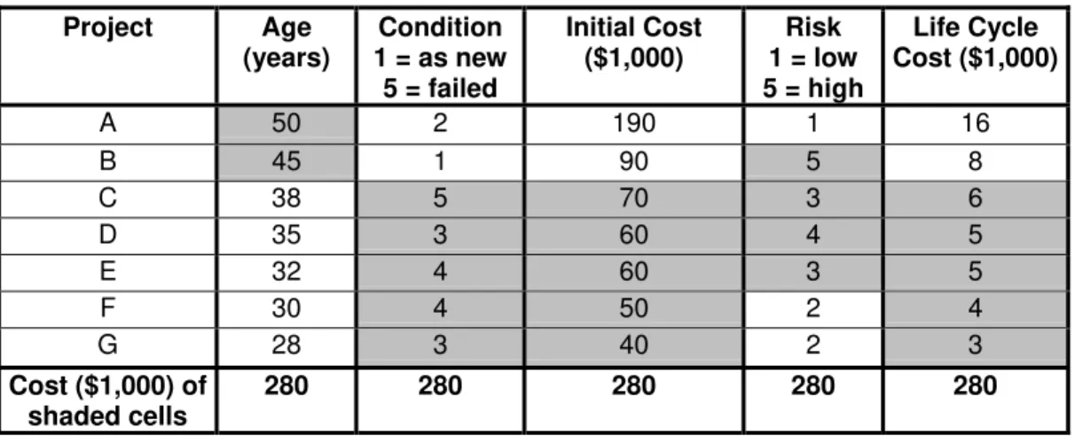
Table 1 illustrates an example in which seven projects (A to G) are to be prioritized. Age-based, condition-Age-based, initial cost-Age-based, risk-Age-based, and life cycle cost-based (LCC) optimization criteria for each of the hypothetical projects are presented and compared in Table 1, more innovative techniques will be illustrated and discussed later in the paper. These five criteria are those typically used in practice for project selection (NAMSG 2004).

Table 1: Selection criteria and maintenance and renewal costs

Project Age (years) Condition 1 = as new 5 = failed Initial Cost ($1,000) Risk 1 = low 5 = high Life Cycle Cost ($1,000) A 50 2 190 1 16 B 45 1 90 5 8 C 38 5 70 3 6 D 35 3 60 4 5 E 32 4 60 3 5 F 30 4 50 2 4 G 28 3 40 2 3 Cost ($1,000) of shaded cells 280 280 280 280 280

Typically, the ratings for each criterion are obtained from the asset management, computerized maintenance management system or GIS system identified in Figure 1(a). For example, the asset age is obtained from the date of construction or date of renewal; the condition is obtained from inspection or determined using deterioration models; the risk represents the product of the probability of failure multiplied by the consequence of failure; the initial cost is the required M & R cost, and the life cycle cost is the present value of the M & R cost and all M & R costs until the end of the asset service life (ASTM 1994).

Prioritization is defined in this paper as the preference ranking of projects. The prioritization for the age-, condition-, risk-, initial cost-, and LCC-based criteria means that the projects having the worst scores for that criterion have the highest priority; that is, oldest first, worst condition first, riskiest first, lowest initial cost first, lowest LCC first.

Further, Table 1 illustrates how each optimization criterion can individually be used to prioritize M & R of projects; that is, the sum of the “Initial Cost” for the highest priority projects in each criterion (shaded cells) equals $280,000.

In our example we assume that the annual maintenance budget is limited to $280,000; however, the total “Initial Cost” of all the projects is double that amount, or $560,000. Therefore, only half the projects can be selected this budget year. The projects with the higher priorities in each selection criterion, and still within the budget, are shaded in Table 1.

In this contrived example, it is easy to see how single criterion prioritization can be conflicting. For example, age-based prioritization (this could be described as data-poor decision-making) selects the oldest assets: -- however, Project A has a very good condition rating (i.e. 2), a low risk of failure (1), and high project cost ($190,000). Using condition-based prioritization (or reactive decision-making), Projects C through G are selected, but Project B is not, -- a relatively old asset with the highest risk. Table 1 clearly shows that age and condition-based prioritization can be diametrically opposite. The risk-based prioritization (i.e. risk-averse decision-making) captures high risk Project B but Project F with a very poor condition rating (4) is not funded. The LCC-based prioritization (i.e. minimize long term expenditures) is theoretically more sustainable than the others; however, similar to the initial cost-based prioritization (last column in Table 1: -- maximize number of projects), it does not capture high risk Project B and includes Project G that is relatively new, in good condition (3), and a moderate risk (2).

MULTIPLE CRITERIA PRIORITIZATION TECHNIQUES

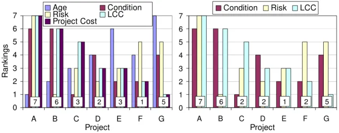
Any number, combination, or weighting of these five criteria can be used for prioritization. For example, Figure 2(a) graphically displays individual rankings for the five criteria from Table 1. Figure 2(b) displays the results of applying equal weights to only the condition, risk and LCC criteria. The numbers above the project name are the sequential ranking of the averages of individual criterion rankings for both Figure 2(a) and (b).

0 1 2 3 4 5 6 7 A B C D E F G R ank ings Age Condition Risk LCC Project Cost 5 1 3 2 3 6 7 0 1 2 3 4 5 6 7 A B C D E F G Condition Risk LCC 5 2 1 2 2 6 7 Project Project

Figure 2: Prioritization for (a) age, condition, risk, LCC and cost (b) condition, risk and LCC.

ANALYTIC HIERARCHY PROCESS (AHP) FOR WEIGHT GENERATION

The analytic hierarchy process (AHP) is a multi-criteria decision-making (MCDM) technique that is used to generate weights (Carlsson and Fullér 1996). AHP uses objective mathematics

5

to process the subjective and personal preferences of an individual or a group in decision-making (ASTM 1995, Saaty 2001). AHP works on a premise that complex problems can be handled by structuring them into a simple and comprehensible hierarchical structure. AHP is performed following these three steps:

(1) structuring of a problem into a hierarchy consisting of a goal and subordinate criteria, (2) establishing pairwise comparisons between elements (criteria) at each level, and (3) synthesizing and establishing the overall priority to rank the alternatives.

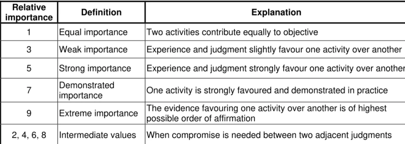
Pairwise comparison is carried out between any two criteria at each level in the hierarchy. The pairwise comparisons range from 1 to 9, where “1” indicates that two criteria are equally important, while the other extreme “9” represents that one criterion is more important than the other, as shown in Table 2. Solution of the AHP hierarchical structure is obtained by synthesizing local and global preference weight to obtain the overall priority (Saaty 1980).

Table 2: AHP pairwise comparison table (Saaty 1980)

Relative

importance Definition Explanation

1 Equal importance Two activities contribute equally to objective

3 Weak importance Experience and judgment slightly favour one activity over another 5 Strong importance Experience and judgment strongly favour one activity over another 7 Demonstrated

importance One activity is strongly favoured and demonstrated in practice 9 Extreme importance The evidence favouring one activity over another is of highest

possible order of affirmation

2, 4, 6, 8 Intermediate values When compromise is needed between two adjacent judgments

In the illustrative example, a simple hierarchical structure is selected: the overall goal is to prioritize maintenance and renewal projects where the subordinate criteria are condition of the asset (Condition), prevalent risk (Risk) and project cost (Cost). This two layer hierarchical structure is a simplistic view of the complex issue of project ranking, as other factors (e.g., municipal objectives, political preference, intervention alternative, etc.) can influence the decision-making. Nevertheless, this hierarchical structure suffices for illustration purposes.

Using actual preference data obtained from participants in a related experiment with the Municipal Infrastructure Investment Planning project (MIIP 2006), a simple pairwise comparison between condition, risk and project cost was obtained (Tesfamariam and Vanier 2005). The three questions presented to the participants (related to project ranking) were:

• What is the level of influence (or dominance) of condition to risk?

• What is the level of influence (or dominance) of condition to project cost? • What is the level of influence (or dominance) of risk to project cost?

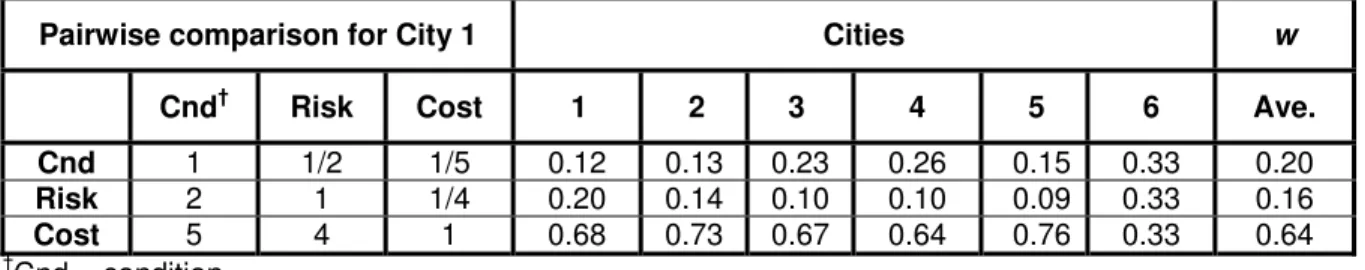
For general illustration, the response for City 1 is shown in Table 3; it can be inferred that the dominance of risk to condition is 2, cost to condition is 5, and cost to risk is 4. Consequently, an arithmetic mean is used to compute the relative importance of each criterion. The final weights computed are wcnd = 0.12, wrisk = 0.20, and wcost = 0.68. The final weights for other cities are summarized in Table 3, as is the average weight of the six cities.

Table 3: AHP weight for the project participants (From Tesfamariam and Vanier 2005)

Pairwise comparison for City 1 Cities w

Cnd† Risk Cost 1 2 3 4 5 6 Ave.

Cnd 1 1/2 1/5 0.12 0.13 0.23 0.26 0.15 0.33 0.20

Risk 2 1 1/4 0.20 0.14 0.10 0.10 0.09 0.33 0.16

Cost 5 4 1 0.68 0.73 0.67 0.64 0.76 0.33 0.64

†_{Cnd = condition}

Finally, once the basic weights and input criteria are identified, the final step of the AHP process is to synthesize through the aforementioned hierarchy. As a result, one can readily see in Table 3 that the three preferences of City 6 are rated equally and differ from the other cities that have similar preferences.

WEIGHTED MEAN (WM)

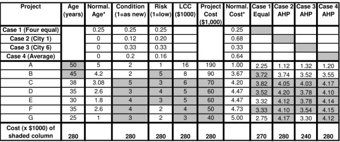
Simple weighted mean can be applied to the selection criteria to demonstrate how AHP weights can be used in alternative prioritization techniques. The basic input criteria shown in Table 1 have been used in conjunction with the AHP weights from Table 3 to produce the different prioritization techniques in Table 4.

Table 4 illustrates the results of four different prioritization techniques. In “Case 1” of Table 4, equal weights (0.25 each) are assigned to the four criteria. Cases 2 to 4 of Table 4 display the AHP weighted results and the shading highlights the highest priority projects whose total cost amounts to less than the allocated budget of $280,000.

This contrived example also highlights the issue of partially funded projects in the prioritization list: -- for Cases 1 and 3 the sum of the highest priority projects is less than the budget of $280K, and the next project(s) will bring that sum over the budget. In fact, for Case 3 the next highest priority is Project B (3.52 rating); however, at $90K it is too expensive, but the next highest rating (Project G - 3.3 rating) at $40 brings the total to $280K. The authors realize that this “fine-tuning” prioritization is typical and controversial in practice but feel it is outside of the scope of this paper.

One can readily see in this illustrative example that priorities can quickly change depending on any number of factors. The different prioritizations in Table 4 show the importance of selecting suitable weights, the significance of the deciding criteria and the contributions of the individual values for each criterion.

7

Table 4: Weighting of prioritization criteria

Project Age (years) Normal. Age* Condition (1=as new) Risk (1=low) LCC ($1000) Project Cost ($1,000) Normal. Cost* Case 1 Equal Case 2 AHP Case 3 AHP Case 4 AHP Case 1 (Four equal) 0.25 0.25 0.25 0.25

Case 2 (City 1) 0 0.12 0.20 0.68 Case 3 (City 6) 0 0.33 0.33 0.33 Case 4 (Average) 0 0.2 0.16 0.64 A 50 5 2 1 16 190 1.00 2.25 1.12 1.32 1.20 B 45 4.2 2 5 8 90 3.67 3.72 3.74 3.52 3.55 C 38 3.08 5 3 6 70 4.20 _{3.82 4.05 4.03 4.17} D 35 2.6 3 4 5 60 4.47 3.52 4.20 3.78 4.10 E 30 1.8 4 3 5 60 4.47 3.32 4.12 3.78 4.14 F 35 2.6 4 2 4 50 4.73 _{3.33 4.10 3.54 4.15} G 25 1 3 2 3 40 5.00 2.75 4.17 3.30 4.12 Cost (x $1000) of shaded column 280 280 280 280 280 270 280 240 280 *It is assumed that Normalized Age and Normalized Cost are linear transformations between the lowest age or cost (value = 1) and highest age or cost (value = 5). It is understood that different linear or geometric transformations are suitable and that many end conditions could be selected.

MULTI-OBJECTIVE OPTIMIZATION (MOO)

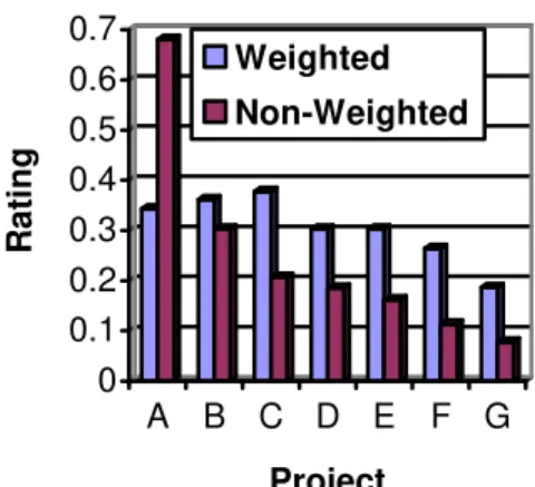
Multi-objective optimization (MOO) is a significantly more sophisticated way to prioritize alternatives. As maintenance management is multi-objective in nature, it requires determination of the optimal maintenance strategy that achieves the best trade-off between several relevant and possibly conflicting criteria. For example, maintenance optimization may seek to satisfy the following three criteria: (a) minimization of costs; (b) maximization of network condition; and (c) minimization of risk of failure (Lounis and Cohn, 1995).

For single-objective optimization problems, the notion of optimality is easily defined as the minimum (or maximum) value of some given objective function. However, the notion of optimality in multi-objective optimization problems is not that obvious. In general, there is no single optimal (or superior) solution that simultaneously yields a minimum (or maximum) for all objective functions. The “Pareto optimum concept” is adopted as the solution to the MOO problem. A solution is said to be a Pareto optimum, if and only if there exists no solution in the feasible domain that may yield an improvement of some objective function without worsening at least another objective function (Lounis and Cohn, 1993; 1995). Typically in a MOO problem, several Pareto optima can be obtained, and the issue is to select the solution that is the best compromise between all competing objectives. Such a solution is referred to as “satisficing” solution in compromise programming literature and yields the minimum distance from a set of Pareto optima to the so-called “ideal solution”. The weighting of the maintenance objectives depends on the attitude of the decision-maker towards the risk of failure, economy, and network reliability. In Figure 3, the results of MOO for non-weighted and weighted multiple-criteria, namely cost, condition and risk are shown. The weights assigned in weighted MOO are the same as those used earlier in Table 3.

0 0.1 0.2 0.3 0.4 0.5 0.6 0.7 Ra ti n g A B C D E F G Project Weighted Non-Weighted

Figure 3: Multi-objective-based maintenance prioritization.

FUZZY SYNTHETIC EVALUATION (FSE)

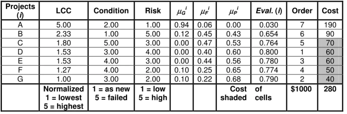
Fuzzy synthetic evaluation (FSE) technique, which is a method based on fuzzy set theory, is employed here for performing MCDM. The term synthetic is used to describe the process of evaluation, whereby several individual elements or components of an evaluation are synthesized into an aggregate form. The underlying fuzzy approach can accommodate both numeric and/or linguistic components. Simple fuzzy classification, fuzzy similarity method and the fuzzy comprehensive assessment, are all derivatives of fuzzy synthetic evaluation (Sadiq and Rodriguez 2004; Rajani et al. 2006). A typical FSE follows a distinct three-step process, namely, fuzzification, aggregation and defuzzification (Sadiq et al. 2004).

Fuzzification of criteria

It is assumed that each and every criterion (i.e. cost, condition state and risk) can be described by n linguistic constants defined over their specific universe of discourse (scale). In this paper, we selected n = 3, corresponding to linguistic constants good, fair, and poor. Table 5 provides the universe of discourse for each criterion ranging over an interval of [1, 5]. Data for each criterion is mapped (or fuzzified). For example, for Project A, the risk value is “1”, which after fuzzification provides a 3-tuple fuzzy set of

(

)

Aggregation of criteria

Relative degrees of importance have to be assigned in order to aggregate criteria. The AHP weights for three criteria are wcos_t = 0.68; wcnd = 0.12; and wrisk = 0.2, as shown in Table 3. The aggregation of criteria is performed using:

(

)

[

]

⎥

⎥

⎥

⎦

⎤

⎢

⎢

⎢

⎣

⎡

•

=

w

w

w

µ

µ

µ

µ

µ

µ

µ

µ

µ

µ

µ

µ

9

where Project (i) = {A, B,…,G and ‘•’ represents matrix multiplication. A 3-tuple fuzzy set

(

)

P i F i

G µ µ

µ represents the aggregated contribution of three criteria (L – life cycle cost, C – condition, and R – risk) in the evaluation of an alternative (i.e., project) “i”.

Defuzzification using quality ordered weights

A process known as defuzzification can be used to calculate the crisp value of a fuzzy set. Many defuzzification techniques are available (Chen and Hwang 1992). A weighted average approach (scoring method) can be used for crisp evaluation by assigning specific quality-ordered weights q to memberships (Lu et al. 1999), for example:

⎟ ⎠ ⎞ ⎜ ⎝ ⎛ ∑ ∗ = = n j j i j q i Eval 1 ) ( . µ (2)

The quality-ordered weights are defined as qi ∈ [0, 1]. For example, for three pre-defined

linguistic constants good, fair, and poor, quality-ordered weights of qG = 0, qF = 0.5 and qP = 1 can be used. The candidate projects are ordered using this crisp evaluation. A higher score means a higher priority for maintenance and renewal.

Table 5: Fuzzy synthetic evaluation (FSE) for project selection

Projects

(i) LCC Condition Risk µG

i

µF i

µP i

Eval. _{(i) Order Cost}

A 5.00 2.00 1.00 0.94 0.06 0.00 0.030 7 190 B 2.33 1.00 5.00 0.12 0.45 0.43 0.654 6 90 C 1.80 5.00 3.00 0.00 0.47 0.53 0.764 5 70 D 1.53 3.00 4.00 0.00 0.40 0.60 0.800 1 60 E 1.53 4.00 3.00 0.00 0.44 0.56 0.780 3 60 F 1.27 4.00 2.00 0.10 0.25 0.65 0.774 4 50 G 1.00 3.00 2.00 0.10 0.22 0.68 0.790 2 40 Normalized 1 = lowest 5 = highest 1 = as new 5 = failed 1 = low 5 = high Cost shaded of cells $1000 280 DISCUSSION

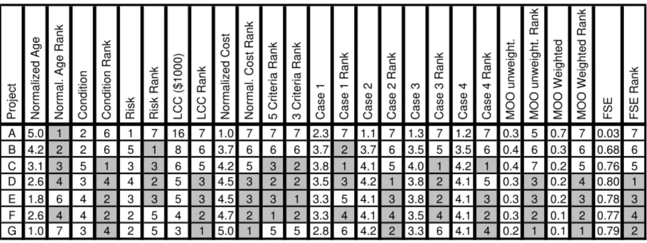
This paper has illustrated a number of prioritization techniques that can be used to rate and rank projects for maintenance and renewal. The different projects used in the illustrative examples are typical of those found in practice and point to the difficult decisions that infrastructure managers must make. The ratings and the rankings for each prioritization technique are summarized in Table 6. It can be readily seen that there can be little correlation between any of these prioritization techniques; in fact, in our example no one project is consistently selected as one of the top four rankings shaded in Table 6.

Intuitively, decision-makers select their preferred alternatives; however, we all have our own biases, and shortcomings. Even with a limited number of projects (i.e. seven), a short selection of decision criteria (i.e. five), and a manageable scale for ratings (i.e. 1 to 5), it is a

daunting task to select the “correct projects” for funding, even for the first year of a strategic plan. Decision-making becomes increasingly more difficult when it involves selecting “correct projects” in future years of a 10 or 20-year strategic plan.

Table 6: Ratings and rankings of M & R projects for illustrative example

Project Normalized Age Normal. Age Rank Condition Condition Rank Ris

k

R

isk R

ank

LCC ($1000) LCC Rank Normalized Cost Norm

al. Cos

t Rank

5 Criteria Rank 3 Criteria Rank Cas

e

1

Case 1 Rank Cas

e

2

Case 2 Rank Cas

e

3

Case 3 Rank Cas

e

4

Case 4 Rank MOO unweight. MOO unweight. Rank MOO Weighted MOO Weighted Rank FSE FSE Rank

A 5.0 1 2 6 1 7 16 7 1.0 7 7 7 2.3 7 1.1 7 1.3 7 1.2 7 0.3 5 0.7 7 0.03 7 B 4.2 2 2 6 5 1 8 6 3.7 6 6 6 3.7 2 3.7 6 3.5 5 3.5 6 0.4 6 0.3 6 0.68 6 C 3.1 3 5 1 3 3 6 5 4.2 5 3 2 3.8 1 4.1 5 4.0 1 4.2 1 0.4 7 0.2 5 0.76 5 D 2.6 4 3 4 4 2 5 3 4.5 3 2 2 3.5 3 4.2 1 3.8 2 4.1 5 0.3 3 0.2 4 0.80 1 E 1.8 6 4 2 3 3 5 3 4.5 3 3 1 3.3 5 4.1 3 3.8 2 4.1 3 0.3 3 0.2 3 0.78 3 F 2.6 4 4 2 2 5 4 2 4.7 2 1 2 3.3 4 4.1 4 3.5 4 4.1 2 0.3 2 0.1 2 0.77 4 G 1.0 7 3 4 2 5 3 1 5.0 1 5 5 2.8 6 4.2 2 3.3 6 4.1 4 0.2 1 0.1 1 0.79 2 One could emphasize the advantages and shortcomings of this or that prioritization technique, or why one project should be selected over another using the data in this illustrative example; but in the end, proper decision-making comes down to having adequate data. It is necessary to have adequate or reliable data to compare various criteria, to state clearly the institutional objectives, to harmonize and normalize data from different sources, to quantify subjective preferences such as risk aversion, and to keep the decision-making strategy consistent over a number of years into the future. Halpern and Fagin (1992) noted that data aggregation is not a problem of mathematics rather it is a problem of judgment! For researchers in the field of decision-making and infrastructure management, there is a lot of work ahead to make this happen.

CONCLUSIONS

This research paper does not attempt to develop models to select the “truly optimal projects” or even to identify the best decision model or prioritization technique; rather, it attempts to illustrate by example the results of specific decision-making paradigms and the poor correlation between these methods or models. Research opportunities in this field of strategic infrastructure management include developing DSS tools that use real or simulation data to demonstrate the pitfalls or advantages of specific decision-making paradigms. In developing such tools, researchers can assist decision-makers to make better decisions, and as a result, to improve the management and the quality of our built environment.

REFERENCES

ASCE (2005). Report Card for America’s Infrastructure, American Society of Civil Engineering (available at www.asce.org/files/pdf/reportcard/2005reportcardpdf.pdf).

11

ASTM (1995). E1765-95-92: Standard Practice for Applying Analytical Hierarchy Process (AHP) to Multiattribute Decision Analysis of Investments Related to Buildings and Building Systems, American Society of Testing Materials, West Conshohocken, PA. ASTM (1994). E917: Standard Practice for Measuring Life-Cycle Costs of Buildings and

Building Systems, American Society for Testing and Materials, West Conshohocken, PA. Carlsson, C. and Fullér, R. (1996). “Fuzzy multiple criteria decision-making: Recent

developments”, Fuzzy Sets and Systems, 78: 139–153.

Chen, S.J. and Hwang, C.L. (1992). Fuzzy Multiple Attribute Decision-Making, Springer-Vaerlag, NY.

Halpern, J.Y., and Fagin, R. (1992). “Two views of belief: belief as generalized probability and belief as evidence”, Artificial Intelligence, 54: 275-317.

Lounis, Z. and Cohn, M.Z. (1993). “Multiobjective Optimization of Prestressed Concrete Structures”, Journal of Structural Engineering, 119(3), pp. 794-808.

Lounis, Z. and Cohn, M.Z. (1995). “An Engineering Approach to Multicriteria Optimization of Highway Bridges”, Journal of Microcomputers in Civil Engineering, 10(4), pp. 233-238.

Lu, R.S., Lo, S.L. and Hu, J.Y. (1999). “Analysis of Reservoir Water Quality using Fuzzy Synthetic Evaluation”, Stochastic Environmental Research and Risk Assessment, 13: 327-336. MIIP (2006). Municipal Infrastructure Investment Planning Project web site, (available at

irc.nrc-cnrc.gc.ca/ui/bu/miip_e.html)

NAMSG (2004). Optimised Decision Making Guidelines: A Sustainable Approach to Managing Infrastructure, Edition 1.0, November, New Zealand National Asset Management Steering Group. Rajani, B., Kleiner, Y. and Sadiq, R. (2006). “Translation of Pipe Inspection Results into

Condition Rating using Fuzzy Synthetic Evaluation Technique”, Journal of Water Supply: Research & Technology – AQUA, 55(1): 11-24.

Saaty, T.L. (1980). The Analytic Hierarchy Process, McGraw-Hill, New York.

Saaty, T.L. (2001). “How to make a Decision?”, Models, Methods, Concepts and Applications of the Analytic Hierarchy Process, Ed. Saaty, T.L., & Vargas, L.G., Kluwer International Series. Sadiq, R. and Rodriguez, M.J. (2004). “Fuzzy Synthetic Evaluation of Disinfection By-Products

– a Risk-Based Indexing System”, Journal of Environmental Management, 73(1): 1-13. Sadiq, R., Rajani, B. and Kleiner, Y. (2004). “A Fuzzy Based Method of Soil Corrosivity Evaluation for

Predicting Water Main Deterioration”, Journal of Infrastructure Systems. ASCE, 10(4): 149-156. Tesfamariam, S. and Vanier, D.J. (2005). “The Analytical Hierarchy Process For Eliciting

Decision Preferences in Asset Management” INFRA 2005 Urban Infrastructure: Managing the Assets, Mastering the Technology, Montréal, November, pp. 1-31, (available at irc.nrc-cnrc.gc.ca/fulltext/nrcc47721).

TRM (2003). Civil Infrastructure Systems: Technology Roadmap, Canadian Society for Civil Engineering, June, 48p., (available at www.csce.ca/TRM/TRM-Report_english_01.pdf). Vanier, D.J. and Rahman, S. (2004). MIIP Report: Survey on Municipal Infrastructure

Assets, Internal Report B-5123.2, Institute for Research in Construction, Ottawa, ON, (available at irc.nrc-cnrc.gc.ca/fulltext/b5123.2).

Vanier, D.J. and Lounis, Z. (2006). “Towards Sustainability and Integration of Civil Infrastructure Management”, Electronic Journal of Information Technology in Construction (ITCon), Special Edition: Decision Support Systems (DSS) for Infrastructure Management, in press.