EUROPEAN ORGANIZATION FOR NUCLEAR RESEARCH (CERN)
CERN-EP-2020-239 LHCb-PAPER-2020-041 April 22, 2021Angular analysis
of the B
+
→ K
∗+
µ
+
µ
−
decay
LHCb collaboration† AbstractWe present an angular analysis of the B+→ K∗+(→ KS0π+)µ+µ− decay using
9 fb−1 of pp collision data collected with the LHCb experiment. For the first time,
the full set of CP -averaged angular observables is measured in intervals of the dimuon invariant mass squared. Local deviations from Standard Model predictions are observed, similar to those in previous LHCb analyses of the isospin-partner
B0→ K∗0µ+µ− decay. The global tension is dependent on which effective couplings
are considered and on the choice of theory nuisance parameters.
Published in Phys. Rev. Lett. 126, 161802 (2021)
© 2021 CERN for the benefit of the LHCb collaboration. CC BY 4.0 licence.
†Authors are listed at the end of this Letter.
Transitions between b quarks and s quarks with the emission of two charged leptons, `+`−, only proceed through loop-level processes. Such decays are therefore sensitive to
possible contributions from heavy mediators that are inaccessible to direct-production searches. Recent studies of b→ s`+`− branching fractions [1–5], angular distributions [1,
4, 6–13] and ratios of branching fractions between decays with different flavours of lepton pairs [14–18] show discrepancies with respect to the predictions of the Standard Model (SM). While these deviations can be consistently explained by the presence of contributions from additional vector or axial-vector currents [19–37], effects from uncertainties related to hadronic form factors or long-distance contributions cannot be ruled out [38–42].
The B→ K∗µ+µ− decay, where K∗ denotes the K∗(892) meson, has been the subject
of extensive studies [7, 12, 43, 44]. A large number of these decays are recorded at the LHC experiments and the flavour of the B meson can be identified from the K∗→ Kπ decay products. This allows the full set of angular observables of the B→ K∗µ+µ− decay
to be studied. A recent study [12] of the B0→ K∗0µ+µ− decay channel by the LHCb
collaboration confirmed the tension in the angular observables with respect to the SM predictions.
This letter reports the first measurement of the complete set of angular observables in the isospin partner decay B+→ K∗+µ+µ−, with the K∗+ meson reconstructed through the
decay chain K∗+→ K0
Sπ+ with KS0→ π+π−. Charge-conjugation is implied throughout
this letter. This decay is mediated by the same underlying processes as the B0→ K∗0µ+µ−
decay, while potentially receiving additional contributions from b→ uW+ transitions,
leading to the emission of a K∗+ meson [45]. Furthermore, any deviation from isospin symmetry, as reported previously in the B→ K∗γ decay [46], could result in a difference
in the angular distributions between the isospin partners. In the SM, however, isospin-breaking effects are expected to be small. The analysis uses the data set collected by the LHCb collaboration in the years 2011, 2012 (Run 1) and 2015–2018 (Run 2), at centre-of-mass energies of 7, 8 and 13 TeV, respectively. The data set corresponds to an integrated luminosity of 9 fb−1.
The LHCb detector [47, 48] is a single-arm forward spectrometer covering the pseudorapidity range 2 < η < 5, designed for the study of particles containing b or c quarks. The detector includes a high-precision tracking system consisting of a silicon-strip vertex detector surrounding the pp interaction region [49], a large-area silicon-silicon-strip detector located upstream of a dipole magnet with a bending power of about 4 Tm, and three stations of silicon-strip detectors and straw drift tubes [50, 51] placed downstream of the magnet. The tracking system provides a measurement of the momentum, p, of charged particles with a relative uncertainty that varies from 0.5% at low momentum to 1.0% at 200 GeV/c. The minimum distance of a track to a primary pp collision vertex (PV), the impact parameter, is measured with a resolution of (15 + 29/pT) µm, where pT
is the component of the momentum transverse to the beam, in GeV/c. Different types of charged hadrons are distinguished using information from two ring-imaging Cherenkov detectors [52]. Photons, electrons and hadrons are identified by a calorimeter system consisting of scintillating-pad and preshower detectors, an electromagnetic and a hadronic calorimeter. Muons are identified by a system composed of alternating layers of iron and multiwire proportional chambers [53]. The online event selection is performed by a trigger [54, 55], which consists of a hardware stage, based on information from the calorimeter and muon systems, followed by a software stage, which applies a full event reconstruction.
Simulated decays are used to model the effects of the reconstruction and the candidate selection. In the simulation, pp collisions are generated using Pythia [56] with a specific LHCb configuration [57]. Decays of unstable particles are described by EvtGen [58], in which final-state radiation is generated using Photos [59]. The interaction of the generated particles with the detector, and its response, are implemented using the Geant4 toolkit [60], as described in Ref. [61]. Corrections to the simulation are applied to account for mismodelling in the pT spectrum of the B+ mesons and the multiplicity of tracks in
the event. The corrections are obtained from a background-subtracted data sample of B+→ (J/ψ → µ+µ−) K∗+ decays.
In the first two stages of the trigger, the event is selected based on kinematical and geometrical properties of the muons. In the last trigger stage, dimuon or topological trigger algorithms are used to select the B+ candidate. The K0
S→ π+π− decays are reconstructed
in two different categories: the long category involves short-lived KS0 candidates for which the pions are reconstructed in the vertex detector; the downstream category comprises K0
S candidates that decay later such that track segments of the pions can only be
reconstructed in tracking detectors downstream of the vertex locator. The KS0 candidates reconstructed in the long category have better mass, momentum and vertex resolution than those in the downstream category, where the latter has a larger sample size than the former. The KS0 candidates are required to have an invariant mass within 30 MeV/c2 of the known K0
S mass [62].
The K∗+→ K0
Sπ+ decay is reconstructed by combining a KS0 candidate with a charged
pion and requiring their invariant mass to be within 100 MeV/c2 of the world average
of the K∗+ mass [62]. The B+→ K∗+µ+µ− candidates are formed by combining the
K∗+ candidate with two well-identified, oppositely charged muons. The B+ candidates
are required to have an invariant mass, m(K0
Sπ+µ+µ−), in the range 5150–6000 MeV/c2.
The lower value of the mass window is chosen to reject background from partially reconstructed B→ K0
Sπ+πµ+µ− decays. Dimuon pairs having invariant mass squared, q2,
around the φ(1020) (0.98 < q2 < 1.1 GeV2/c4), J/ψ (8.0 < q2 < 11.0 GeV2/c4) and ψ(2S)
(12.5 < q2 < 15.0 GeV2/c4) resonances are vetoed. All tracks in the final state are required
to have a significant impact parameter with respect to any PV and the B+ candidate
decay vertex needs to be well displaced from any PV in the event. A kinematical fit [63] is performed to the full decay chain, in which the reconstructed K0
S mass is constrained
to the known value [62].
Decays of B0 mesons to the K0
Sµ+µ− final state with a pion added can form a
peaking structure in the B+ mass window. Therefore, candidates with an invariant
mass m(K0
Sµ+µ−) within 50 MeV/c2 of the known B0 mass are vetoed. Background
originating from B+→ (J/ψ → µ+µ−) K∗+ decays is probed by testing the K0
Sπ+ and
dimuon invariant masses formed by exchanging the particle hypotheses between the pion from the K∗+ meson decay and the muon with the same charge. The candidates with a
dimuon mass within 50 MeV/c2 of the J/ψ meson mass and a K0
Sπ+ invariant mass within
30 MeV/c2 of the K∗+ mass are then rejected. The background from B decays with two
hadrons misidentified as muons is negligible.
To increase the signal-to-background ratio, a multivariate classification is employed. The data are split into four subsets, according to the Run 1 and Run 2 data-taking periods and the category of the K0
S meson. A boosted decision tree with gradient boosting [64, 65]
from the TMVA toolkit [66] is then trained on each data set individually, using simulated events as a proxy for signal and candidates with m(K0
m(K0 Sπ +µ+µ−) [ MeV/c2] 5200 5400 5600 5800 6000 Candidates / (8 .5 Me V /c 2 ) 0 100 200
LHCb
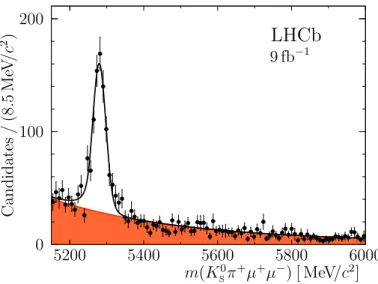
9 fb−1 1Figure 1: Distribution of the KS0π+µ+µ− invariant mass. The black points represent the full
data set, while the solid curve shows the fit result. The background component is represented by the orange shaded area.
as a proxy for background. The variables include kinematical and topological properties of the final state or intermediate particles, the quality of the vertex of the B+ candidate, and an isolation criterion related to the asymmetry in pT between all tracks inside a
cone around the flight directions of the B+ candidates and the tracks associated to the
B+ decay products [67]. Figure 1 shows the B+-candidate invariant mass distribution,
m(K0
Sπ+µ+µ−), for all the selected data. A fit model with a double-sided Crystal Ball
function for the signal and an exponential function for the background component is overlaid. The number of B+→ K∗+µ+µ−signal candidates from this fit is 737± 34, where
the uncertainty is statistical only.
Ignoring the natural width of the K∗+ meson, the decay B+→ K∗+µ+µ− can be fully
described by four variables: q2 and the set of three angles ~Ω = (θ
`, θK, φ). The angle
between the µ+ (µ−) and the direction opposite to that of the B+ (B−) in the rest frame
of the dimuon system is denoted θ`. The angle between the direction of the KS0 and the
B+ (B−) in the rest frame of the K∗+ (K∗−) system is denoted θ
K. The angle φ is the
angle between the plane defined by the momenta of the muon pair and the plane defined by the kaon and pion momenta in the B+ (B−) rest frame. A full description of the
angular basis is given in Ref. [44].
Averaging over B+ and B− decays, with rates respectively denoted Γ and ¯Γ, the
differential decay rate of the B+→ K∗+µ+µ− decay with the K0
Sπ+ system in a P-wave
1 d(Γ + ¯Γ)/dq2 d4(Γ + ¯Γ) dq2d~Ω P = 9 32π h 3 4(1− FL) sin 2θ K + FLcos2θK +14(1− FL) sin2θKcos 2θ`
−FLcos2θKcos 2θ`+ S3sin2θKsin2θ`cos 2φ
+S4sin 2θKsin 2θ`cos φ + S5sin 2θKsin θ`cos φ
+43AFBsin2θKcos θ`+ S7sin 2θKsin θ`sin φ
+S8sin 2θKsin 2θ`sin φ + S9sin2θKsin2θ`sin 2φ
i ,
(1)
where FL is the fraction of the longitudinally polarised K∗+ mesons, AFB is the
forward-backward asymmetry of the dimuon system and Si are other CP -averaged observables [7].
The K0
Sπ+system can also be in an S-wave configuration, which modifies the differential
decay rate to 1 d(Γ + ¯Γ)/dq2 d4(Γ + ¯Γ) dq2d~Ω P+S = (1− FS) 1 d(Γ + ¯Γ)/dq2 d4(Γ + ¯Γ) dq2d~Ω P + 3 16πFSsin 2θ l + 9 32π(S11+ S13cos 2θl) cos θK + 9
32π(S14sin 2θl+ S15sin θl) sin θKcos φ
+ 9
32π(S16sin θl+ S17sin 2θl) sin θKsin φ , (2)
where FS denotes the S-wave fraction and the coefficients S11, S13–S17 arise from
in-terference between the S- and P-wave amplitudes. Throughout this letter, FS and the
interference coefficients are treated as nuisance parameters. In addition to the observable basis comprising FL, AFB and S3–S9, a basis with so-called optimised observables, denoted
Pi(0), for which the leading form-factor uncertainties cancel [68], is used. The notation for the Pi(0) observables is defined in Ref. [43].
Due to the limited number of signal candidates, the observables cannot all be measured simultaneously. A folding procedure is therefore employed that uses symmetries of the differential decay rate in the angles to cancel some observables, reducing the number of free parameters in the fit. By performing different folds, all angular observables can be studied, without any loss in precision. Five different folds are used to study the observables AFB
and S9 (P2 and P3), S4 (P40), S5 (P50), S7 (P60) and S8 (P80), respectively. The observables
FL and S3 (P1) are measured in each fold. This procedure is detailed in Ref. [69] and was
previously used in Refs. [8–10, 43, 44]. The values of FL and S3 (P1) are taken from the
same fold that is used to extract the value of S8 (P80), as the number of free parameters in
the fit is the smallest in this fold.
The angular observables are extracted using an unbinned maximum-likelihood fit to the B+ candidate mass and the three decay angles in intervals of q2. The eight narrow and two
wide q2 intervals are identical to those in Refs. [7, 12]. The angular distributions are fitted
with the function described in Eq. (2) for the signal, and with second-order polynomials in cos θK and cos θ` for the background. The background in the φ angle is uniform. No
significant correlation is observed between the angular background distributions in the B+ candidate mass sidebands, justifying a factorisation of the background description in
the three decay angles.
The reconstruction and selection efficiency varies over the angular and q2 phase space.
This acceptance effect is parametrised before folding using the sum over the product of four one-dimensional Legendre polynomials, each depending on one angle or q2. This
is analogous to the procedure used in Ref. [12]. The effect is corrected using weights derived from simulation. The weight then corresponds to the inverse of the efficiency. No dependence of the acceptance effect on the K∗+ candidate mass is observed.
Given the low signal yield and narrow q2 intervals, the S-wave fraction FS cannot
be determined with sufficient precision to guarantee unbiased results for the P-wave angular observables. Therefore, a two-dimensional unbinned maximum-likelihood fit to m(KS0π+µ+µ−) and the K∗+ candidate mass m(KS0π+) is first performed in three q2 intervals: 1.1–8.0, 11.0–12.5 and 15.0–19.0 GeV2/c4. The m(K0
Sπ+µ+µ−) distribution is
fitted using the signal and background model described above. The K∗+ candidate mass is fitted using a relativistic Breit-Wigner function to describe the P-wave component, the LASS parametrisation to describe the S-wave component [70] and a linear function to describe the combinatorial background. S- and P-wave interference terms are neglected in this treatment. The value of FS in the default narrow q2 intervals is then computed by
multiplying the value of FS in the broad intervals with the ratio between FL in the narrow
and broad intervals. This procedure assumes a similar q2 dependence of the longitudinal
component of the P wave and the S wave and is broadly compatible with the results from Ref. [5]. Given the weak dependence of the P-wave observables on the value of FS,
this procedure ensures unbiased results without relying on values of FS from an external
measurement. Pseudoexperiments indicate that determining FS in this manner induces
at most a bias of 13% of the statistical uncertainty on the angular observables. This is treated as a systematic uncertainty. All values of FS are measured to be positive and
compatible with the results in Ref. [5].
Fitting the folded data set only provides statistical correlations between observables measured in the same fold. In order to obtain the correlations between all observables, the bootstrapping technique [71] is used to produce a large number of pseudodata sets. The measurement of the observables in each fold of these pseudodata sets enables computing the correlations between observables in different folds. The statistical precision of the elements of the correlation matrix is determined to be around 0.11. In order to ensure correct coverage in the presence of physical boundaries of the observables, the statistical uncertainty for each observable in each q2 interval for the signal channel is evaluated using
the Feldman-Cousins technique [72].
The full analysis procedure with acceptance correction, extraction of FS and extraction
of the angular observables, is tested on a sample of B+→ J/ψK∗+ decays with the same
selection as applied to the signal channel, but requiring the dimuon invariant mass squared to be in the range 8.68–10.09 GeV2/c4. The results are found to be in good agreement
with previous measurements from the BaBar [73], Belle [74] and LHCb [75] experiments. Several sources of systematic uncertainties are considered and their sizes are estimated using pseudoexperiments. Various contributions to the overall systematic uncertainty
are related to the correction of acceptance effects. They include the limited size of the simulation sample and the parametrisation of the acceptance function. Other systematic uncertainties are related to the correction of differences between data and simulation, the model of the B+ candidate mass distribution and angular background, the impact of
the B0→ K0
Sµ+µ− veto on the mass distribution of the combinatorial background, the
angular resolution and the effect of constraining the value of FS with a two-dimensional fit.
Pseudoexperiments are used to assess a possible bias introduced by the fit procedure. The pseudodata samples are generated based on the result of the fit to data or on the predictions from either the SM or a new physics scenario favoured by the LHCb measurement from Ref. [12] with the real part of the Wilson coefficient C9 shifted by −1 with respect to SM
predictions. Here, C9 is the strength of the vector coupling in an effective field theory of b
quark to s quark transitions. The largest bias observed is 33% of the statistical uncertainty for S4 in the q2 interval 4.0–6.0 GeV2/c4. Given that the biases can depend on the values
of the observables themselves, the largest biases observed among the three pseudodata samples are taken as systematic uncertainties. The potential exchange of the π+ mesons
from the decays of the K∗+ and KS0 candidates and the angular background description differing between the upper and lower mass sidebands are both considered as further sources of systematic uncertainty. Both effects are found to be negligible. All systematic uncertainties are added in quadrature and their total size is reported together with the numerical results of the observables in Sec. 2 of the Supplemental Material. A summary of the contributions from the various sources is given in Table 23 of the Supplemental Material. The statistical uncertainty dominates for all q2 intervals and all observables,
which implies that correlations with the results from Ref. [12] are negligible.
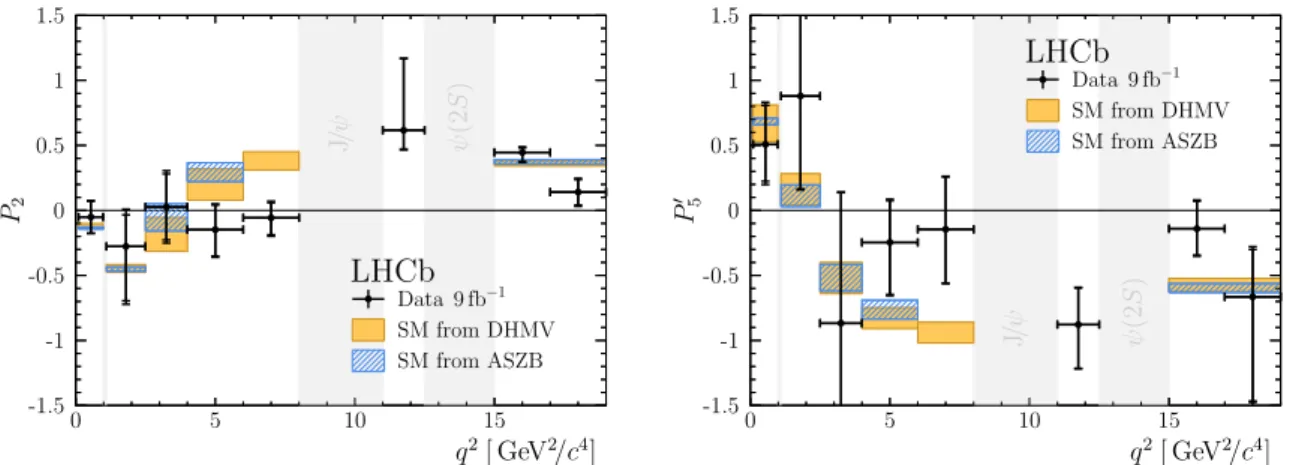
The results of the angular fits for the observables P2 = 23AFB/(1− FL) and
P0
5 = S5/pFL(1− FL) are shown in Fig. 2. They are compared with the two SM
pre-dictions taken from Ref. [76] with hadronic form factors from Refs. [77–79], and from Refs. [80, 81] with hadronic form factors from Ref. [82]. The rest of the observables are presented in Figs. 3 and 4 in the Supplemental Material to this letter. The numerical results of the angular fits to the data are presented in Tables 1 and 2, where values for the two wide q2 intervals are also given. The correlations are given in Tables 3–12 and
13–22 for the Si and Pi(0) observables, respectively.
The majority of observables show good agreement with the SM predictions, FL and
AFB agree well with the measurements in Ref. [13]. The largest local discrepancy is in the
measurement of P2 in the 6.0–8.0 GeV2/c4 interval, where a deviation of 3.0σ with respect
to the SM prediction is observed. The pattern of deviations from the SM predictions in the observables S5 (P50) and AFB (P2) broadly agrees with the deviations observed in the
B0→ K∗0µ+µ− channel.
The Flavio package [83] (version 2.0.0) is used to perform a fit to the angular observables varying the parameter Re(C9), which is motivated by Refs. [7, 12]. In order
to minimise the theoretical uncertainties related to contributions from virtual charm-quark loops [82] and broad charmonium resonances [84–86], the narrow q2 intervals up
to 6.0 GeV2/c4 plus the wide q2 interval 15.0 < q2 < 19.0 GeV2/c4 are included in the fit.
The default Flavio SM nuisance parameters are used, including form-factor parameters and subleading corrections to account for long-distance QCD interference effects with the charmonium decay modes [76, 77]. The best-fit point results in a shift with respect to the SM value of Re(C9) of −1.9 and gives a tension with the SM of 3.1σ. However,
q2[ GeV2/c4] 0 5 10 15 P2 -1.5 -1 -0.5 0 0.5 1 1.5 J/ ψ ψ (2 S ) Data 9 fb−1 SM from DHMV SM from ASZB LHCb 1 q2[ GeV2/c4] 0 5 10 15 P 0 5 -1.5 -1 -0.5 0 0.5 1 1.5 J/ ψ ψ (2 S ) Data 9 fb−1 SM from DHMV SM from ASZB LHCb 1
Figure 2: The CP -averaged observables (left) P2 and (right) P50 in intervals of q2. The first
(second) error bars represent the statistical (total) uncertainties. The theoretical predictions in blue are based on Ref. [76] with hadronic form factors taken from Refs. [77–79] and are obtained with the Flavio software package [83] (version 2.0.0). The theoretical predictions in orange are based on Refs. [80, 81] with hadronic form factors from Ref. [82]. The grey bands indicate the regions of excluded φ(1020), J/ψ and ψ(2S) resonances.
varied and the handling of the SM nuisance parameters.
In summary, using the complete pp data set collected with the LHCb experiment in Runs 1 and 2, the full set of angular observables for the decay B+→ K∗+µ+µ− is
measured for the first time. The results confirm the global tension with respect to the SM predictions previously reported in the decay B0→ K∗0µ+µ−.
Acknowledgements
We express our gratitude to our colleagues in the CERN accelerator departments for the excellent performance of the LHC. We thank the technical and administrative staff at the LHCb institutes. We acknowledge support from CERN and from the national agencies: CAPES, CNPq, FAPERJ and FINEP (Brazil); MOST and NSFC (China); CNRS/IN2P3 (France); BMBF, DFG and MPG (Germany); INFN (Italy); NWO (Netherlands); MNiSW and NCN (Poland); MEN/IFA (Romania); MSHE (Russia); MICINN (Spain); SNSF and SER (Switzerland); NASU (Ukraine); STFC (United Kingdom); DOE NP and NSF (USA). We acknowledge the computing resources that are provided by CERN, IN2P3 (France), KIT and DESY (Germany), INFN (Italy), SURF (Netherlands), PIC (Spain), GridPP (United Kingdom), RRCKI and Yandex LLC (Russia), CSCS (Switzerland), IFIN-HH (Romania), CBPF (Brazil), PL-GRID (Poland) and OSC (USA). We are indebted to the communities behind the multiple open-source software packages on which we depend. Individual groups or members have received support from AvH Foundation (Germany); EPLANET, Marie Sk lodowska-Curie Actions and ERC (European Union); A*MIDEX, ANR, Labex P2IO and OCEVU, and R´egion Auvergne-Rhˆone-Alpes (France); Key Research Program of Frontier Sciences of CAS, CAS PIFI, CAS CCEPP, Fundamental Research Funds for the Central Universities, and Sci. & Tech. Program of Guangzhou (China); RFBR, RSF and Yandex LLC (Russia); GVA, XuntaGal and GENCAT (Spain);
Supplemental Material
This supplemental material includes additional information to that already provided in the main letter.
The full set of results for both sets of angular observables is presented in graphical form in Sec. 1 and in tabular form in Sec. 2. The correlations between the angular observables are given in Sec. 3 and Sec. 4 for Si and Pi(0) observables, respectively. A summary of the
systematic uncertainties is given in Sec. 5. The signal yields in each q2 interval are given
in Table 24. The projections of the data in m(K0
Sπ+µ+µ−), cos θK, cos θ` and φ using the
angular fold with the transformation φ→ φ + π, for φ < 0, are given in Figs. 5 - 8 along with the fitted probability density functions.
1
Graphical results for the S
iand P
(0)
q2[ GeV2/c4] 0 5 10 15 FL 0 0.5 1 J/ ψ ψ (2 S ) Data 9 fb−1 SM from ASZB LHCb 1 q2[ GeV2/c4] 0 5 10 15 S3 -1 -0.5 0 0.5 1 J/ ψ ψ (2 S ) Data 9 fb−1 SM from ASZB LHCb 1 q2[ GeV2/c4] 0 5 10 15 S4 -1 -0.5 0 0.5 1 J/ ψ ψ (2 S ) Data 9 fb−1 SM from ASZB LHCb 1 q2[ GeV2/c4] 0 5 10 15 S5 -1 -0.5 0 0.5 1 J/ ψ ψ (2 S ) Data 9 fb−1 SM from ASZB LHCb 1 q2[ GeV2/c4] 0 5 10 15 AFB -1 -0.5 0 0.5 1 J/ ψ ψ (2 S ) Data 9 fb−1 SM from ASZB LHCb 1 q2[ GeV2/c4] 0 5 10 15 S7 -1 -0.5 0 0.5 1 J/ ψ ψ (2 S ) Data 9 fb−1 SM from ASZB LHCb 1 q2[ GeV2/c4] 0 5 10 15 S8 -1 -0.5 0 0.5 1 J/ ψ ψ (2 S ) Data 9 fb−1 SM from ASZB LHCb 1 q2[ GeV2/c4] 0 5 10 15 S9 -1 -0.5 0 0.5 1 J/ ψ ψ (2 S ) Data 9 fb−1 SM from ASZB LHCb 1
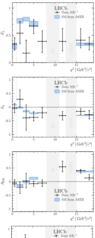
Figure 3: The CP -averaged observables FL, AFB and S3–S9 versus q2. The first (second) error
bars represent the statistical (total) uncertainties. The theoretical predictions are based on Refs. [76–79]. The grey bands indicate regions of excluded resonances.
q2[ GeV2/c4] 0 5 10 15 FL 0 0.5 1 J/ ψ ψ (2 S ) Data 9 fb−1 SM from ASZB LHCb 1 q2[ GeV2/c4] 0 5 10 15 P1 -1.5 -1 -0.5 0 0.5 1 1.5 J/ ψ ψ (2 S ) Data 9 fb−1 SM from DHMV SM from ASZB LHCb 1 q2[ GeV2/c4] 0 5 10 15 P2 -1.5 -1 -0.5 0 0.5 1 1.5 J/ ψ ψ (2 S ) Data 9 fb−1 SM from DHMV SM from ASZB LHCb 1 q2[ GeV2/c4] 0 5 10 15 P3 -1.5 -1 -0.5 0 0.5 1 1.5 J/ ψ ψ (2 S ) Data 9 fb−1 SM from DHMV SM from ASZB LHCb 1 q2[ GeV2/c4] 0 5 10 15 P 0 4 -1.5 -1 -0.5 0 0.5 1 1.5 J/ ψ ψ (2 S ) Data 9 fb−1 SM from DHMV SM from ASZB LHCb 1 q2[ GeV2/c4] 0 5 10 15 P 0 5 -1.5 -1 -0.5 0 0.5 1 1.5 J/ ψ ψ (2 S ) Data 9 fb−1 SM from DHMV SM from ASZB LHCb 1 q2[ GeV2/c4] 0 5 10 15 P 0 6 -1.5 -1 -0.5 0 0.5 1 1.5 J/ ψ ψ (2 S ) Data 9 fb−1 SM from DHMV SM from ASZB LHCb 1 q2[ GeV2/c4] 0 5 10 15 P 0 8 -1.5 -1 -0.5 0 0.5 1 1.5 J/ ψ ψ (2 S ) Data 9 fb−1 SM from DHMV SM from ASZB LHCb 1
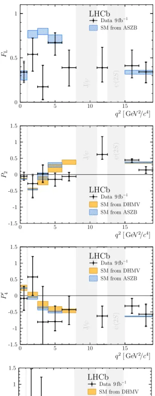
Figure 4: The optimised observables P1 to P80 versus q2. The first (second) error bars represent
the statistical (total) uncertainties. The theoretical predictions are based on Refs. [80–82] (orange) and on Refs. [76–79] (blue). The grey bands indicate regions of excluded resonances.
2
Tabular results for the S
iand P
i(0)observables
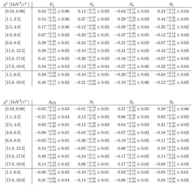
Table 1: Results for the CP -averaged observables FL, AFB and S3–S9. The first uncertainties
are statistical and the second systematic.
q2 [ GeV2 /c4] F L S3 S4 S5 [0.10, 0.98] 0.34+0.10 −0.10± 0.06 0.14 +0.15 −0.14± 0.02 −0.04 +0.17 −0.16± 0.04 0.24 +0.12 −0.15± 0.04 [1.1, 2.5] 0.54+0.21 −0.18± 0.06 0.37+0.97−0.41± 0.03 0.29+0.34−0.27± 0.03 0.44+0.38−0.32± 0.05 [2.5, 4.0] 0.17+0.23 −0.32± 0.06 −0.12+0.66−0.39± 0.02 −0.39+0.48−0.45± 0.04 −0.35+0.41−0.31± 0.02 [4.0, 6.0] 0.67+0.12−0.14± 0.02 −0.20 +0.16 −0.19± 0.01 −0.37 +0.20 −0.13± 0.05 −0.12 +0.14 −0.19± 0.03 [6.0, 8.0] 0.39+0.20−0.21± 0.01 −0.24 +0.18 −0.17± 0.02 −0.21 +0.20 −0.18± 0.02 −0.07 +0.16 −0.20± 0.02 [11.0, 12.5] 0.39+0.24−0.17± 0.02 −0.10 +0.13 −0.13± 0.02 −0.31 +0.14 −0.17± 0.02 −0.43 +0.14 −0.16± 0.02 [15.0, 17.0] 0.41+0.21−0.14± 0.02 −0.26 +0.12 −0.11± 0.03 −0.16 +0.10 −0.11± 0.02 −0.07 +0.10 −0.10± 0.03 [17.0, 19.0] 0.34+0.12 −0.11± 0.03 −0.13 +0.20 −0.17± 0.04 −0.27 +0.14 −0.15± 0.06 −0.32 +0.16 −0.34± 0.04 [1.1, 6.0] 0.59+0.09 −0.09± 0.03 −0.10+0.11−0.11± 0.01 −0.20+0.13−0.14± 0.03 −0.04+0.12−0.12± 0.02 [15.0, 19.0] 0.40+0.13−0.11± 0.03 −0.21 +0.09 −0.09± 0.03 −0.19 +0.10 −0.13± 0.06 −0.12 +0.07 −0.07± 0.02 q2 [ GeV2/c4] AFB S7 S8 S9 [0.10, 0.98] −0.05+0.12 −0.12± 0.03 −0.01+0.19−0.17± 0.01 0.21+0.22−0.20± 0.05 0.28+0.15−0.12± 0.06 [1.1, 2.5] −0.21+0.19−0.23± 0.04 0.15 +0.32 −0.72± 0.02 0.06 +0.40 −0.37± 0.04 0.05 +0.37 −0.30± 0.02 [2.5, 4.0] 0.03+0.28−0.26± 0.01 −0.15 +0.49 −0.69± 0.03 0.04 +0.75 −0.58± 0.03 0.31 +0.39 −0.36± 0.02 [4.0, 6.0] −0.08+0.09 −0.10± 0.01 −0.04 +0.18 −0.20± 0.01 −0.07 +0.21 −0.22± 0.03 −0.18 +0.22 −0.33± 0.02 [6.0, 8.0] −0.05+0.11 −0.12± 0.01 −0.36 +0.18 −0.15± 0.02 −0.19 +0.18 −0.16± 0.02 −0.11 +0.21 −0.20± 0.02 [11.0, 12.5] 0.54+0.21−0.18± 0.05 −0.05 +0.14 −0.14± 0.01 0.06 +0.14 −0.14± 0.01 0.19 +0.24 −0.19± 0.03 [15.0, 17.0] 0.40+0.04 −0.09± 0.01 −0.24 +0.11 −0.11± 0.02 −0.17 +0.12 −0.11± 0.02 0.14 +0.12 −0.09± 0.02 [17.0, 19.0] 0.14+0.12 −0.07± 0.02 0.06 +0.16 −0.16± 0.01 0.17 +0.18 −0.16± 0.02 −0.08 +0.15 −0.15± 0.02 [1.1, 6.0] −0.08+0.07 −0.08± 0.02 −0.10 +0.11 −0.13± 0.01 0.02 +0.13 −0.14± 0.02 −0.05 +0.11 −0.12± 0.01 [15.0, 19.0] 0.31+0.06−0.06± 0.04 −0.14 +0.08 −0.09± 0.01 −0.06 +0.09 −0.09± 0.01 0.04 +0.08 −0.06± 0.02
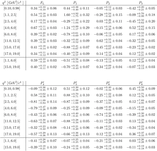
Table 2: Results for the optimised observables FL and P1–P80. The first uncertainties are
statistical and the second systematic.
q2 [ GeV2/c4] F L P1 P2 P3 [0.10, 0.98] 0.34+0.10 −0.10± 0.06 0.44 +0.38 −0.40± 0.11 −0.05 +0.12 −0.12± 0.03 −0.42 +0.20 −0.21± 0.05 [1.1, 2.5] 0.54+0.18 −0.19± 0.03 1.60 +4.92 −1.75± 0.32 −0.28 +0.24 −0.42± 0.15 −0.09 +0.70 −0.99± 0.18 [2.5, 4.0] 0.17+0.24 −0.14± 0.04 −0.29 +1.43 −1.04± 0.22 0.03 +0.26 −0.25± 0.11 −0.45 +0.50 −0.62± 0.20 [4.0, 6.0] 0.67+0.11 −0.14± 0.03 −1.24 +0.99 −1.17± 0.29 −0.15 +0.19 −0.20± 0.06 0.52 +0.82 −0.62± 0.15 [6.0, 8.0] 0.39+0.20 −0.21± 0.02 −0.78+0.61−0.69± 0.10 −0.06+0.12−0.13± 0.05 0.17+0.33−0.31± 0.06 [11.0, 12.5] 0.39+0.23 −0.16± 0.03 −0.32+0.44−0.52± 0.09 0.62+0.55−0.14± 0.04 −0.32+0.29−0.65± 0.05 [15.0, 17.0] 0.41+0.18−0.14± 0.02 −0.88 +0.41 −0.67± 0.07 0.45 +0.03 −0.07± 0.03 −0.23 +0.16 −0.20± 0.02 [17.0, 19.0] 0.34+0.11−0.12± 0.04 −0.40 +0.58 −0.57± 0.09 0.14 +0.10 −0.10± 0.04 0.12 +0.21 −0.21± 0.02 [1.1, 6.0] 0.59+0.10 −0.10± 0.03 −0.51 +0.56 −0.54± 0.08 −0.13 +0.13 −0.13± 0.05 0.12 +0.27 −0.28± 0.04 [15.0, 19.0] 0.40+0.13 −0.11± 0.02 −0.70 +0.35 −0.43± 0.07 0.34 +0.09 −0.07± 0.04 −0.07 +0.12 −0.13± 0.03 q2 [ GeV2/c4] P0 4 P50 P60 P80 [0.10, 0.98] −0.09+0.36 −0.35± 0.12 0.51 +0.30 −0.28± 0.12 −0.02 +0.40 −0.34± 0.06 0.45 +0.50 −0.39± 0.09 [1.1, 2.5] 0.58+0.62 −0.56± 0.11 0.88 +0.70 −0.71± 0.10 0.25 +1.22 −1.32± 0.08 0.12 +0.75 −0.76± 0.05 [2.5, 4.0] −0.81+1.09 −0.84± 0.14 −0.87+1.00−1.68± 0.09 −0.37+1.59−3.91± 0.05 0.12+7.89−4.95± 0.07 [4.0, 6.0] −0.79+0.47 −0.28± 0.09 −0.25+0.32−0.40± 0.09 −0.09+0.40−0.41± 0.05 −0.15+0.44−0.48± 0.05 [6.0, 8.0] −0.43+0.41−0.45± 0.06 −0.15 +0.40 −0.41± 0.06 −0.74 +0.29 −0.40± 0.03 −0.39 +0.30 −0.39± 0.02 [11.0, 12.5] −0.63+0.30 −0.34± 0.07 −0.88 +0.28 −0.34± 0.05 −0.11 +0.28 −0.29± 0.03 0.13 +0.29 −0.30± 0.04 [15.0, 17.0] −0.32+0.23 −0.22± 0.08 −0.14 +0.21 −0.20± 0.06 −0.48 +0.21 −0.21± 0.02 −0.34 +0.23 −0.22± 0.04 [17.0, 19.0] −0.57+0.29 −0.36± 0.13 −0.66 +0.36 −0.80± 0.13 0.12 +0.33 −0.33± 0.04 0.36 +0.37 −0.33± 0.07 [1.1, 6.0] −0.41+0.28 −0.28± 0.07 −0.07+0.25−0.25± 0.04 −0.21+0.23−0.23± 0.04 0.03+0.26−0.28± 0.06 [15.0, 19.0] −0.39+0.18 −0.21± 0.10 −0.24+0.16−0.16± 0.05 −0.28+0.19−0.14± 0.03 −0.11+0.19−0.18± 0.03
3
Correlation matrices for the S
iobservables
Correlation matrices between the CP -averaged observables FL, AFB and S3–S9 in the
different q2 intervals are provided in Tables 3–12. Correlations between observables
measured with different folds are obtained using the bootstrapping technique [71]. The different q2 intervals are statistically independent.
Table 3: Correlation matrix for the CP -averaged observables FL, AFB and S3–S9 from the
maximum-likelihood fit in the interval 0.10 < q2 <0.98 GeV2/c4.
FL S3 S4 S5 AFB S7 S8 S9 FL 1 0.04 −0.01 0.03 0.04 0.12 −0.00 −0.11 S3 1 −0.02 0.12 −0.02 0.02 0.06 0.02 S4 1 −0.27 −0.09 −0.25 0.24 −0.06 S5 1 0.10 0.22 −0.18 0.06 AFB 1 0.19 −0.27 −0.06 S7 1 −0.35 0.22 S8 1 −0.08 S9 1
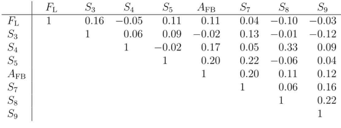
Table 4: Correlation matrix for the CP -averaged observables FL, AFB and S3–S9 from the
maximum-likelihood fit in the interval 1.1 < q2<2.5 GeV2/c4.
FL S3 S4 S5 AFB S7 S8 S9 FL 1 0.16 −0.05 0.11 0.11 0.04 −0.10 −0.03 S3 1 0.06 0.09 −0.02 0.13 −0.01 −0.12 S4 1 −0.02 0.17 0.05 0.33 0.09 S5 1 0.20 0.22 −0.06 0.04 AFB 1 0.20 0.11 0.12 S7 1 0.06 0.16 S8 1 0.22 S9 1
Table 5: Correlation matrix for the CP -averaged observables FL, AFB and S3–S9 from the
maximum-likelihood fit in the interval 2.5 < q2<4.0 GeV2/c4.
FL S3 S4 S5 AFB S7 S8 S9 FL 1 0.02 −0.01 0.06 −0.08 −0.02 −0.07 0.04 S3 1 0.02 −0.06 −0.01 −0.03 0.07 0.02 S4 1 0.00 −0.06 0.10 −0.05 −0.00 S5 1 0.01 −0.07 0.00 −0.11 AFB 1 0.05 0.06 −0.16 S7 1 0.26 −0.14 S8 1 −0.09 S9 1
Table 6: Correlation matrix for the CP -averaged observables FL, AFB and S3–S9 from the
maximum-likelihood fit in the interval 4.0 < q2<6.0 GeV2/c4.
FL S3 S4 S5 AFB S7 S8 S9 FL 1 0.20 −0.09 −0.09 0.07 0.01 0.16 −0.03 S3 1 −0.08 −0.10 0.03 0.11 0.17 0.03 S4 1 −0.08 −0.15 0.07 −0.04 0.05 S5 1 −0.17 −0.02 0.09 −0.02 AFB 1 −0.04 −0.03 −0.01 S7 1 0.09 0.09 S8 1 −0.08 S9 1
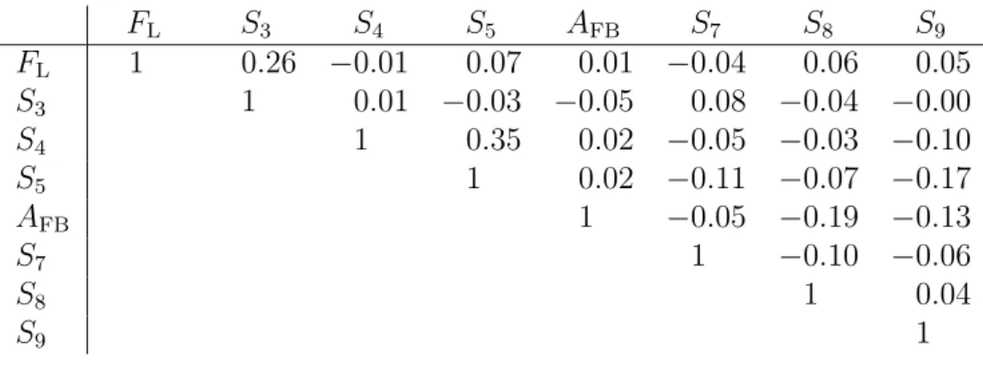
Table 7: Correlation matrix for the CP -averaged observables FL, AFB and S3–S9 from the
maximum-likelihood fit in the interval 6.0 < q2<8.0 GeV2/c4.
FL S3 S4 S5 AFB S7 S8 S9 FL 1 0.26 −0.01 0.07 0.01 −0.04 0.06 0.05 S3 1 0.01 −0.03 −0.05 0.08 −0.04 −0.00 S4 1 0.35 0.02 −0.05 −0.03 −0.10 S5 1 0.02 −0.11 −0.07 −0.17 AFB 1 −0.05 −0.19 −0.13 S7 1 −0.10 −0.06 S8 1 0.04 S9 1
Table 8: Correlation matrix for the CP -averaged observables FL, AFB and S3–S9 from the
maximum-likelihood fit in the interval 11.0 < q2 <12.5 GeV2/c4.
FL S3 S4 S5 AFB S7 S8 S9 FL 1 0.09 0.03 0.09 −0.44 −0.09 −0.13 −0.08 S3 1 −0.08 −0.13 −0.08 −0.04 −0.04 −0.19 S4 1 0.08 0.06 −0.05 −0.09 0.12 S5 1 −0.30 0.05 −0.04 −0.10 AFB 1 0.10 0.11 0.15 S7 1 0.05 −0.07 S8 1 −0.07 S9 1
Table 9: Correlation matrix for the CP -averaged observables FL, AFB and S3–S9 from the
maximum-likelihood fit in the interval 15.0 < q2 <17.0 GeV2/c4.
FL S3 S4 S5 AFB S7 S8 S9 FL 1 0.19 0.04 0.07 −0.28 −0.06 −0.13 −0.07 S3 1 −0.09 −0.06 0.04 0.01 −0.06 0.01 S4 1 0.27 0.07 0.10 0.06 0.14 S5 1 −0.15 0.09 −0.06 −0.13 AFB 1 0.07 −0.02 0.16 S7 1 0.23 0.02 S8 1 0.00 S9 1
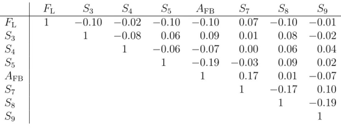
Table 10: Correlation matrix for the CP -averaged observables FL, AFB and S3–S9 from the
maximum-likelihood fit in the interval 17.0 < q2 <19.0 GeV2/c4.
FL S3 S4 S5 AFB S7 S8 S9 FL 1 −0.10 −0.02 −0.10 −0.10 0.07 −0.10 −0.01 S3 1 −0.08 0.06 0.09 0.01 0.08 −0.02 S4 1 −0.06 −0.07 0.00 0.06 0.04 S5 1 −0.19 −0.03 0.09 0.02 AFB 1 0.17 0.01 −0.07 S7 1 −0.17 0.10 S8 1 −0.19 S9 1
Table 11: Correlation matrix for the CP -averaged observables FL, AFB and S3–S9 from the
maximum-likelihood fit in the interval 1.1 < q2<6.0 GeV2/c4.
FL S3 S4 S5 AFB S7 S8 S9 FL 1 0.17 −0.00 −0.02 0.01 0.04 0.08 0.06 S3 1 −0.01 −0.02 −0.02 0.04 −0.03 −0.05 S4 1 −0.03 0.06 −0.02 0.19 −0.01 S5 1 0.01 0.14 0.04 0.04 AFB 1 −0.05 0.04 0.05 S7 1 0.17 −0.02 S8 1 −0.01 S9 1
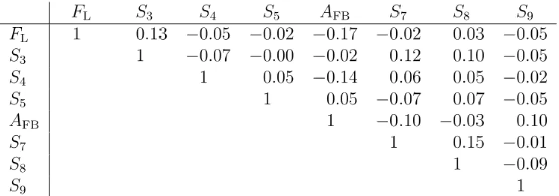
Table 12: Correlation matrix for the CP -averaged observables FL, AFB and S3–S9 from the
maximum-likelihood fit in the interval 15.0 < q2 <19.0 GeV2/c4.
FL S3 S4 S5 AFB S7 S8 S9 FL 1 0.13 −0.05 −0.02 −0.17 −0.02 0.03 −0.05 S3 1 −0.07 −0.00 −0.02 0.12 0.10 −0.05 S4 1 0.05 −0.14 0.06 0.05 −0.02 S5 1 0.05 −0.07 0.07 −0.05 AFB 1 −0.10 −0.03 0.10 S7 1 0.15 −0.01 S8 1 −0.09 S9 1
4
Correlation matrices for the P
i(0)observables
Correlation matrices between the CP -averaged observables Pi in the different q2 intervals
are provided in Tables 13–22. Correlations between observables measured with different folds are obtained using using the bootstrapping technique [71]. The different q2 intervals
are statistically independent.
Table 13: Correlation matrix for the CP -averaged observables FL and Pi(0) from the
maximum-likelihood fit in the interval 0.10 < q2<0.98 GeV2/c4.
FL P1 P2 P3 P40 P50 P60 P80 FL 1 −0.14 0.02 −0.18 −0.03 0.00 0.12 −0.01 P1 1 −0.00 −0.01 −0.03 0.17 0.01 0.03 P2 1 0.02 −0.08 0.09 0.19 −0.24 P3 1 0.06 −0.03 −0.21 0.04 P0 4 1 −0.22 −0.23 0.15 P0 5 1 0.18 −0.18 P60 1 −0.25 P0 8 1
Table 14: Correlation matrix for the CP -averaged observables FL and Pi(0) from the
maximum-likelihood fit in the interval 1.1 < q2 <2.5 GeV2/c4.
FL P1 P2 P3 P40 P50 P60 P80 FL 1 0.03 0.02 −0.01 −0.06 −0.01 0.05 −0.08 P1 1 −0.05 −0.01 0.06 −0.09 −0.03 0.04 P2 1 −0.05 0.15 0.12 0.10 0.13 P3 1 −0.08 −0.07 −0.02 −0.13 P40 1 0.03 −0.01 0.22 P0 5 1 0.09 −0.08 P0 6 1 −0.01 P80 1
Table 15: Correlation matrix for the CP -averaged observables FL and Pi(0) from the
maximum-likelihood fit in the interval 2.5 < q2 <4.0 GeV2/c4.
FL P1 P2 P3 P40 P50 P60 P80 FL 1 0.00 0.00 0.02 −0.02 −0.03 −0.06 −0.03 P1 1 0.00 0.04 0.04 0.00 −0.04 −0.06 P2 1 0.07 −0.01 0.04 0.04 −0.03 P3 1 −0.03 0.02 0.06 −0.01 P40 1 0.07 0.06 0.08 P0 5 1 −0.02 −0.09 P0 6 1 0.21 P80 1
Table 16: Correlation matrix for the CP -averaged observables FL and Pi(0) from the
maximum-likelihood fit in the interval 4.0 < q2 <6.0 GeV2/c4.
FL P1 P2 P3 P40 P50 P60 P80 FL 1 0.16 −0.10 0.02 −0.02 −0.08 0.02 0.08 P1 1 −0.03 0.02 −0.08 0.03 0.03 0.08 P2 1 0.04 −0.12 −0.14 −0.03 −0.05 P3 1 −0.02 −0.02 −0.05 0.09 P40 1 −0.11 −0.01 −0.10 P0 5 1 −0.04 0.07 P0 6 1 0.05 P80 1
Table 17: Correlation matrix for the CP -averaged observables FL and Pi(0) from the
maximum-likelihood fit in the interval 6.0 < q2 <8.0 GeV2/c4.
FL P1 P2 P3 P40 P50 P60 P80 FL 1 0.11 −0.10 0.01 −0.03 0.05 −0.05 −0.00 P1 1 −0.04 0.01 0.01 −0.02 0.02 −0.06 P2 1 0.12 −0.01 0.02 −0.05 −0.17 P3 1 0.04 0.12 0.00 −0.04 P40 1 0.25 −0.03 −0.01 P0 5 1 −0.08 −0.06 P0 6 1 −0.05 P80 1
Table 18: Correlation matrix for the CP -averaged observables FL and Pi(0) from the
maximum-likelihood fit in the interval 11.0 < q2<12.5 GeV2/c4.
FL P1 P2 P3 P40 P50 P60 P80 FL 1 −0.05 0.35 −0.09 0.00 0.04 −0.06 −0.14 P1 1 −0.05 0.17 −0.09 −0.14 −0.03 −0.02 P2 1 −0.15 0.12 −0.14 −0.00 0.07 P3 1 −0.09 0.06 0.07 0.09 P40 1 0.04 −0.03 −0.10 P0 5 1 0.05 −0.01 P0 6 1 0.06 P80 1
Table 19: Correlation matrix for the CP -averaged observables FL and Pi(0) from the
maximum-likelihood fit in the interval 15.0 < q2<17.0 GeV2/c4.
FL P1 P2 P3 P40 P50 P60 P80 FL 1 0.07 0.15 −0.09 0.08 0.09 0.00 −0.09 P1 1 0.01 −0.05 0.00 −0.01 −0.00 −0.06 P2 1 −0.23 0.10 −0.06 0.07 −0.03 P3 1 −0.15 0.10 −0.03 0.02 P40 1 0.27 0.09 0.05 P0 5 1 0.09 −0.07 P0 6 1 0.21 P80 1
Table 20: Correlation matrix for the CP -averaged observables FL and Pi(0) from the
maximum-likelihood fit in the interval 17.0 < q2<19.0 GeV2/c4.
FL P1 P2 P3 P40 P50 P60 P80 FL 1 −0.10 0.09 0.07 0.02 −0.10 0.06 −0.08 P1 1 0.06 0.04 −0.10 0.02 −0.01 0.06 P2 1 0.07 −0.07 −0.16 0.13 −0.00 P3 1 −0.08 0.03 −0.08 0.17 P40 1 −0.08 −0.03 0.05 P0 5 1 0.00 0.08 P0 6 1 −0.12 P80 1
Table 21: Correlation matrix for the CP -averaged observables FL and Pi(0) from the
maximum-likelihood fit in the interval 1.1 < q2 <6.0 GeV2/c4.
FL P1 P2 P3 P40 P50 P60 P80 FL 1 0.11 −0.19 0.01 −0.01 −0.02 0.02 0.08 P1 1 −0.05 0.07 0.01 −0.01 0.00 −0.04 P2 1 −0.06 0.04 0.00 −0.05 0.01 P3 1 0.01 −0.04 0.01 0.01 P0 4 1 −0.03 −0.02 0.18 P50 1 0.14 0.04 P0 6 1 0.17 P0 8 1
Table 22: Correlation matrix for the CP -averaged observables FL and Pi(0) from the
maximum-likelihood fit in the interval 15.0 < q2<19.0 GeV2/c4.
FL P1 P2 P3 P40 P50 P60 P80 FL 1 −0.00 0.03 −0.01 0.00 0.01 0.03 0.05 P1 1 0.01 0.04 −0.06 0.04 0.03 0.08 P2 1 −0.07 −0.13 −0.00 −0.12 −0.03 P3 1 0.03 0.04 0.02 0.08 P0 4 1 −0.00 0.12 0.04 P0 5 1 −0.09 0.07 P60 1 0.17 P0 8 1
5
Systematic uncertainties
The systematic uncertainties are determined for each observable in each q2 interval.
Table 23 summarises the sizes of the systematic effects by giving the maximum value for each systematic uncertainty studied.
The larger systematic uncertainties of the Pi(0) observables compared to the Si
observ-ables arise due to an additional scale factor in the definition of the Pi(0) observables, which depends on the value of FL for a given q2 interval.
Table 23: Maximum values for each source of systematic uncertainty.
Source FL AFB S3–S9 P1 P2–P80
Size of the simulation sample < 0.03 < 0.03 < 0.04 < 0.06 < 0.08 Data-simulation differences < 0.04 < 0.01 < 0.04 < 0.13 < 0.17 Acceptance polynomial order < 0.05 < 0.04 < 0.06 < 0.09 < 0.10 S-wave fraction constraint < 0.05 < 0.02 < 0.03 < 0.13 < 0.14
m(K0
Sπ+µ+µ−) model < 0.01 < 0.01 < 0.01 < 0.06 < 0.02
Peaking background veto < 0.01 < 0.01 < 0.01 < 0.07 < 0.04 Angular resolution < 0.01 < 0.01 < 0.01 < 0.01 < 0.01 Background model < 0.01 < 0.01 < 0.02 < 0.06 < 0.12 Trigger simulation < 0.01 < 0.01 < 0.01 < 0.03 < 0.03 Fit bias at best-fit values < 0.04 < 0.05 < 0.05 < 0.28 < 0.13
6
Yields of signal candidates per q
2interval
Table 24: Yields of signal candidates in the ten q2 intervals. They are obtained from extended
maximum-likelihood fits to the m(KS0π+µ+µ−) distribution. The total number corresponds to
the sum of the eight nominal q2 intervals.
q2 [ GeV2 /c4 ] Signal yield [0.1, 0.98] 102± 12 [1.1, 2.5] 49± 10 [2.5, 4.0] 42± 10 [4.0, 6.0] 109± 13 [6.0, 8.0] 105± 14 [11.0, 12.5] 111± 13 [15.0, 17.0] 144± 13 [17.0, 19.0] 76± 10 [1.1, 6.0] 200± 19 [15.0, 19.0] 220± 17 Total 737± 34
7
Projections of data and fit model
m(K0 Sπ +µ+µ−) [ MeV/c2] 5200 5400 5600 5800 6000 Candidates / (17 Me V /c 2) 0 20 40 LHCb 9 fb −1 0.10 < q2< 0.98 GeV2/c4 1 m(K0 Sπ +µ+µ−) [ MeV/c2] 5200 5400 5600 5800 6000 Candidates / (17 Me V /c 2) 0 10 20 LHCb 9 fb−1 1.10 < q2< 2.50 GeV2/c4 1 m(K0 Sπ +µ+µ−) [ MeV/c2] 5200 5400 5600 5800 6000 Candidates / (17 Me V /c 2) 0 10 20 LHCb 9 fb−1 2.50 < q2< 4.00 GeV2/c4 1 m(K0 Sπ +µ+µ−) [ MeV/c2] 5200 5400 5600 5800 6000 Candidates / (17 Me V /c 2) 0 20 40 LHCb 9 fb−1 4.00 < q2< 6.00 GeV2/c4 1 m(K0 Sπ +µ+µ−) [ MeV/c2] 5200 5400 5600 5800 6000 Candidates / (17 Me V /c 2) 0 20 40 60 LHCb 9 fb−1 6.00 < q2< 8.00 GeV2/c4 1 m(K0 Sπ +µ+µ−) [ MeV/c2] 5200 5400 5600 5800 6000 Candidates / (17 Me V /c 2) 0 20 40 60 LHCb 9 fb−1 11.00 < q2< 12.50 GeV2/c4 1 m(K0 Sπ +µ+µ−) [ MeV/c2] 5200 5400 5600 5800 6000 Candidates / (17 Me V /c 2) 0 20 40 60 15.00 < qLHCb 9 fb2< 17.00 GeV−1 2/c4 1 m(K0 Sπ +µ+µ−) [ MeV/c2] 5200 5400 5600 5800 6000 Candidates / (17 Me V /c 2) 0 10 20 30 17.00 < qLHCb 9 fb2< 19.00 GeV−1 2/c4 1 m(K0 Sπ +µ+µ−) [ MeV/c2] 5200 5400 5600 5800 6000 Candidates / (17 Me V /c 2) 0 50 100 LHCb 9 fb−1 1.10 < q2< 6.00 GeV2/c4 1 m(K0 Sπ +µ+µ−) [ MeV/c2] 5200 5400 5600 5800 6000 Candidates / (17 Me V /c 2) 0 50 100 LHCb 9 fb−1 15.00 < q2< 19.00 GeV2/c4 1Figure 5: Projections for the invariant mass m(KS0π+µ+µ−) in the ten q2 intervals. The black
points represent the data, while the solid curve shows the fit result. The background component is represented by the orange shaded area.
cos θK -1 -0.5 0 0.5 1 W eigh ted candidates / 0. 1 0 10 20 30 LHCb 9 fb−1 0.10 < q2< 0.98 GeV2/c4 1 cos θK -1 -0.5 0 0.5 1 W eigh ted candidates / 0. 1 0 5 10 15 20 LHCb 9 fb−1 1.10 < q2< 2.50 GeV2/c4 1 cos θK -1 -0.5 0 0.5 1 W eigh ted candidates / 0. 1 0 5 10 15 20 LHCb 9 fb−1 2.50 < q2< 4.00 GeV2/c4 1 cos θK -1 -0.5 0 0.5 1 W eigh ted candidates / 0. 1 0 10 20 30 LHCb 9 fb−1 4.00 < q2< 6.00 GeV2/c4 1 cos θK -1 -0.5 0 0.5 1 W eigh ted candidates / 0. 1 0 10 20 30 LHCb 9 fb−1 6.00 < q2< 8.00 GeV2/c4 1 cos θK -1 -0.5 0 0.5 1 W eigh ted candidates / 0. 1 0 10 20 30 LHCb 9 fb−1 11.00 < q2< 12.50 GeV2/c4 1 cos θK -1 -0.5 0 0.5 1 W eigh ted candidates / 0. 1 0 10 20 LHCb 9 fb −1 15.00 < q2< 17.00 GeV2/c4 1 cos θK -1 -0.5 0 0.5 1 W eigh ted candidates / 0. 1 0 5 10 15 LHCb 9 fb−1 17.00 < q2< 19.00 GeV2/c4 1 cos θK -1 -0.5 0 0.5 1 W eigh ted candidates / 0. 1 0 20 40 LHCb 9 fb −1 1.10 < q2< 6.00 GeV2/c4 1 cos θK -1 -0.5 0 0.5 1 W eigh ted candidates / 0. 1 0 10 20 30 LHCb 9 fb−1 15.00 < q2< 19.00 GeV2/c4 1
Figure 6: Projections for the angle cos θK in the ten q2 intervals. The black points represent the
data, while the solid curve shows the fit result. The background component is represented by
the orange shaded area. The invariant mass m(KS0π+µ+µ−) is required to be within 50 MeV/c2
cos θ` -1 -0.5 0 0.5 1 W eigh ted candidates / 0. 1 0 10 20 30 LHCb 9 fb−1 0.10 < q2< 0.98 GeV2/c4 1 cos θ` -1 -0.5 0 0.5 1 W eigh ted candidates / 0. 1 0 5 10 15 20 LHCb 9 fb−1 1.10 < q2< 2.50 GeV2/c4 1 cos θ` -1 -0.5 0 0.5 1 W eigh ted candidates / 0. 1 0 5 10 15 20 LHCb 9 fb−1 2.50 < q2< 4.00 GeV2/c4 1 cos θ` -1 -0.5 0 0.5 1 W eigh ted candidates / 0. 1 0 10 20 30 LHCb 9 fb−1 4.00 < q2< 6.00 GeV2/c4 1 cos θ` -1 -0.5 0 0.5 1 W eigh ted candidates / 0. 1 0 10 20 30 LHCb 9 fb−1 6.00 < q2< 8.00 GeV2/c4 1 cos θ` -1 -0.5 0 0.5 1 W eigh ted candidates / 0. 1 0 10 20 30 LHCb 9 fb−1 11.00 < q2< 12.50 GeV2/c4 1 cos θ` -1 -0.5 0 0.5 1 W eigh ted candidates / 0. 1 0 10 20 LHCb 9 fb −1 15.00 < q2< 17.00 GeV2/c4 1 cos θ` -1 -0.5 0 0.5 1 W eigh ted candidates / 0. 1 0 5 10 15 LHCb 9 fb−1 17.00 < q2< 19.00 GeV2/c4 1 cos θ` -1 -0.5 0 0.5 1 W eigh ted candidates / 0. 1 0 20 40 LHCb 9 fb −1 1.10 < q2< 6.00 GeV2/c4 1 cos θ` -1 -0.5 0 0.5 1 W eigh ted candidates / 0. 1 0 10 20 30 LHCb 9 fb−1 15.00 < q2< 19.00 GeV2/c4 1
Figure 7: Projections for the angle cos θ` in the ten q2 intervals. The black points represent the
data, while the solid curve shows the fit result. The background component is represented by
the orange shaded area. The invariant mass m(KS0π+µ+µ−) is required to be within 50 MeV/c2
φ [ rad] 0 π 2 π W eigh ted candidates / π 10 rad 0 20 40 60 LHCb 9 fb−1 0.10 < q2< 0.98 GeV2/c4 1 φ [ rad] 0 π 2 π W eigh ted candidates / π 10 rad 0 10 20 30 40 LHCb 9 fb−1 1.10 < q2< 2.50 GeV2/c4 1 φ [ rad] 0 π 2 π W eigh ted candidates / π 10 rad 0 10 20 30 40 LHCb 9 fb−1 2.50 < q2< 4.00 GeV2/c4 1 φ [ rad] 0 π 2 π W eigh ted candidates / π 10 rad 0 20 40 60 LHCb 9 fb−1 4.00 < q2< 6.00 GeV2/c4 1 φ [ rad] 0 π 2 π W eigh ted candidates / π 10 rad 0 20 40 60 LHCb 9 fb−1 6.00 < q2< 8.00 GeV2/c4 1 φ [ rad] 0 π 2 π W eigh ted candidates / π 10 rad 0 20 40 60 LHCb 9 fb−1 11.00 < q2< 12.50 GeV2/c4 1 φ [ rad] 0 π 2 π W eigh ted candidates / π 10 rad 0 20 40 LHCb 9 fb −1 15.00 < q2< 17.00 GeV2/c4 1 φ [ rad] 0 π 2 π W eigh ted candidates / π 10 rad 0 10 20 30 LHCb 9 fb−1 17.00 < q2< 19.00 GeV2/c4 1 φ [ rad] 0 π 2 π W eigh ted candidates / π 10 rad 0 50 100 LHCb 9 fb−1 1.10 < q2< 6.00 GeV2/c4 1 φ [ rad] 0 π 2 π W eigh ted candidates / π 10 rad 0 20 40 60 LHCb 9 fb−1 15.00 < q2< 19.00 GeV2/c4 1
Figure 8: Projections for the angle φ in the ten q2 intervals. The black points represent the
data, while the solid curve shows the fit result. The background component is represented by
the orange shaded area. The invariant mass m(KS0π+µ+µ−) is required to be within 50 MeV/c2
References
[1] BaBar collaboration, B. Aubert et al., Measurements of branching fractions, rate asym-metries, and angular distributions in the rare decays B → K`+`− and B → K∗`+`−,
Phys. Rev. D73 (2006) 092001, arXiv:hep-ex/0604007.
[2] LHCb collaboration, R. Aaij et al., Differential branching fractions and isospin asymmetries of B→ K(∗)µ+µ− decays, JHEP 06 (2014) 133, arXiv:1403.8044.
[3] LHCb collaboration, R. Aaij et al., Differential branching fraction and angular analysis of Λ0
b→ Λµ+µ− decays, JHEP 06 (2015) 115, Erratum ibid. 09 (2018) 145,
arXiv:1503.07138.
[4] LHCb collaboration, R. Aaij et al., Angular analysis and differential branching fraction of the decay B0
s→ φµ+µ−, JHEP 09 (2015) 179, arXiv:1506.08777.
[5] LHCb collaboration, R. Aaij et al., Measurements of the S-wave fraction in B0→ K+π−µ+µ− decays and theB0→ K∗(892)0µ+µ− differential branching fraction,
JHEP 11 (2016) 047, Erratum ibid. 04 (2017) 142, arXiv:1606.04731.
[6] CDF collaboration, T. Aaltonen et al., Measurements of the angular distribu-tions in the decays B → K(∗)µ+µ− at CDF, Phys. Rev. Lett. 108 (2012) 081807,
arXiv:1108.0695.
[7] LHCb collaboration, R. Aaij et al., Angular analysis of the B0→ K∗0µ+µ− decay
using 3 fb−1 of integrated luminosity, JHEP 02 (2016) 104, arXiv:1512.04442. [8] Belle collaboration, S. Wehle et al., Lepton-flavor-dependent angular analysis of
B → K∗`+`−, Phys. Rev. Lett. 118 (2017) 111801, arXiv:1612.05014.
[9] CMS collaboration, A. M. Sirunyan et al., Measurement of angular parameters from the decay B0→ K∗0µ+µ− in proton-proton collisions at √s = 8 TeV, Phys. Lett.
B781 (2018) 517, arXiv:1710.02846.
[10] ATLAS collaboration, M. Aaboud et al., Angular analysis of B0
d → K∗µ+µ− decays
in pp collisions at √s = 8 TeV with the ATLAS detector, JHEP 10 (2018) 047, arXiv:1805.04000.
[11] LHCb collaboration, R. Aaij et al., Angular moments of the decay Λ0
b→ Λµ+µ− at
low hadronic recoil, JHEP 09 (2018) 146, arXiv:1808.00264.
[12] LHCb collaboration, R. Aaij et al., Measurement of CP -averaged observables in the B0→ K∗0µ+µ− decay, Phys. Rev. Lett. 125 (2020) 011802, arXiv:2003.04831.
[13] CMS collaboration, A. M. Sirunyan et al., Angular analysis of the decay B+ →
K∗(892)+µ+µ− in proton-proton collisions at √s = 8 TeV, arXiv:2010.13968.
[14] BaBar collaboration, J. P. Lees et al., Measurement of branching fractions and rate asymmetries in the rare decays B → K(∗)`+`−, Phys. Rev. D86 (2012) 032012,
[15] LHCb collaboration, R. Aaij et al., Test of lepton universality with B0→ K∗0`+`−
decays, JHEP 08 (2017) 055, arXiv:1705.05802.
[16] LHCb collaboration, R. Aaij et al., Search for lepton-universality violation in B+→ K+`+`− decays, Phys. Rev. Lett. 122 (2019) 191801, arXiv:1903.09252.
[17] Belle collaboration, S. Choudhury et al., Test of lepton flavor universality and search for lepton flavor violation in B → K`` decays, arXiv:1908.01848, submitted to JHEP.
[18] Belle collaboration, S. Wehle et al., Test of lepton-flavor universality in B → K∗`+`−
decays at belle, arXiv:1904.02440, submitted to Phys. Rev. Lett.
[19] W. Altmannshofer, S. Gori, M. Pospelov, and I. Yavin, Quark flavor transitions in Lµ− Lτ models, Phys. Rev. D89 (2014) 095033, arXiv:1403.1269.
[20] G. Hiller and M. Schmaltz, RK and futureb→ s`` physics beyond the standard model
opportunities, Phys. Rev. D90 (2014) 054014, arXiv:1408.1627.
[21] B. Gripaios, M. Nardecchia, and S. A. Renner, Composite leptoquarks and anomalies in B-meson decays, JHEP 05 (2015) 006, arXiv:1412.1791.
[22] I. de Medeiros Varzielas and G. Hiller, Clues for flavor from rare lepton and quark decays, JHEP 06 (2015) 072, arXiv:1503.01084.
[23] A. Crivellin, G. D’Ambrosio, and J. Heeck, Explaining h → µ±τ∓, B → K∗µ+µ−
and B → Kµ+µ−/B → Ke+e− in a two-Higgs-doublet model with gauged L
µ− Lτ,
Phys. Rev. Lett. 114 (2015) 151801, arXiv:1501.00993.
[24] A. Celis, J. Fuentes-Mart´ın, M. Jung, and H. Serˆodio, Family nonuniversal Z0
models with protected flavor-changing interactions, Phys. Rev. D92 (2015) 015007, arXiv:1505.03079.
[25] A. Falkowski, M. Nardecchia, and R. Ziegler, Lepton flavor non-universality in B-meson decays from a U (2) flavor model, JHEP 11 (2015) 173, arXiv:1509.01249. [26] R. Barbieri, C. W. Murphy, and F. Senia, B-decay anomalies in a composite leptoquark
model, Eur. Phys. J. C77 (2017) 8, arXiv:1611.04930.
[27] A. Crivellin, D. M¨uller, and T. Ota, Simultaneous explanation of R(D(∗)) and b→ sµ+µ−: the last scalar leptoquarks standing, JHEP 09 (2017) 040,
arXiv:1703.09226.
[28] F. Sala and D. M. Straub, A new light particle in B decays?, Phys. Lett. B774 (2017) 205, arXiv:1704.06188.
[29] P. Ko, Y. Omura, Y. Shigekami, and C. Yu, LHCb anomaly and B physics in flavored Z0 models with flavored Higgs doublets, Phys. Rev. D95 (2017) 115040, arXiv:1702.08666.
[30] J.-H. Sheng, R.-M. Wang, and Y.-D. Yang, Scalar leptoquark effects in the lepton flavor violating exclusive b → s`−i `+j decays, Int. J. Theor. Phys. 58 (2019) 480,
[31] G. Hiller, D. Loose, and I. Ni˘sand˘zi´c, Flavorful leptoquarks at hadron colliders, Phys. Rev. D97 (2018) 075004, arXiv:1801.09399.
[32] M. Alguer´o et al., Emerging patterns of new physics with and without Lepton flavour universal contributions, Eur. Phys. J. C79 (2019) 714, arXiv:1903.09578.
[33] J. Aebischer et al., B-decay discrepancies after Moriond 2019, Eur. Phys. J. C80 (2020) 252, arXiv:1903.10434.
[34] A. Arbey et al., Update on the b→ s anomalies, Phys. Rev. D100 (2019) 015045, arXiv:1904.08399.
[35] M. Ciuchini et al., New physics in b→ s`+`− confronts new data on lepton universality,
Eur. Phys. J. C79 (2019) 719, arXiv:1903.09632.
[36] K. Kowalska, D. Kumar, and E. M. Sessolo, Implications for new physics in b→ sµµ transitions after recent measurements by Belle and LHCb, Eur. Phys. J. C79 (2019) 840, arXiv:1903.10932.
[37] A. K. Alok, A. Dighe, S. Gangal, and D. Kumar, Continuing search for new physics in b → sµµ decays: Two operators at a time, JHEP 06 (2019) 089, arXiv:1903.09617. [38] S. J¨ager and J. Martin Camalich, Reassessing the discovery potential of the
B → K∗`+`− decays in the large-recoil region: SM challenges and BSM
opportu-nities, Phys. Rev. D93 (2016) 014028, arXiv:1412.3183.
[39] J. Lyon and R. Zwicky, Resonances gone topsy turvy - the charm of QCD or new physics in b→ s`+`−?, arXiv:1406.0566.
[40] M. Ciuchini et al., B → K∗`+`− decays at large recoil in the Standard Model: a
theoretical reappraisal, JHEP 06 (2016) 116, arXiv:1512.07157.
[41] C. Bobeth, M. Chrzaszcz, D. van Dyk, and J. Virto, Long-distance effects in B → K∗``
from analyticity, Eur. Phys. J. C78 (2018) 451, arXiv:1707.07305.
[42] N. Gubernari, D. van Dyk, and J. Virto, Non-local matrix elements in B(s) →
{K(∗), φ}`+`−, JHEP 02 (2021) 088, arXiv:2011.09813.
[43] LHCb collaboration, R. Aaij et al., Measurement of form-factor-independent observables in the decay B0→ K∗0µ+µ−, Phys. Rev. Lett. 111 (2013) 191801,
arXiv:1308.1707.
[44] LHCb collaboration, R. Aaij et al., Differential branching fraction and angular analysis of the decay B0→ K∗0µ+µ−, JHEP 08 (2013) 131, arXiv:1304.6325.
[45] P. Ball, G. W. Jones, and R. Zwicky, B → V γ beyond QCD factorization, Phys. Rev. D75 (2007) 054004, arXiv:hep-ph/0612081v3.
[46] Belle collaboration, T. Horiguchi et al., Evidence for Isospin Violation and Measure-ment of CP Asymmetries in B → K∗(892)γ, Phys. Rev. Lett. 119 (2017) 191802,
[47] LHCb collaboration, A. A. Alves Jr. et al., The LHCb detector at the LHC, JINST 3 (2008) S08005.
[48] LHCb collaboration, R. Aaij et al., LHCb detector performance, Int. J. Mod. Phys. A30 (2015) 1530022, arXiv:1412.6352.
[49] R. Aaij et al., Performance of the LHCb Vertex Locator, JINST 9 (2014) P09007, arXiv:1405.7808.
[50] R. Arink et al., Performance of the LHCb Outer Tracker, JINST 9 (2014) P01002, arXiv:1311.3893.
[51] P. d’Argent et al., Improved performance of the LHCb Outer Tracker in LHC Run 2, JINST 12 (2017) P11016, arXiv:1708.00819.
[52] M. Adinolfi et al., Performance of the LHCb RICH detector at the LHC, Eur. Phys. J. C73 (2013) 2431, arXiv:1211.6759.
[53] A. A. Alves Jr. et al., Performance of the LHCb muon system, JINST 8 (2013) P02022, arXiv:1211.1346.
[54] R. Aaij et al., The LHCb trigger and its performance in 2011, JINST 8 (2013) P04022, arXiv:1211.3055.
[55] R. Aaij et al., Performance of the LHCb trigger and full real-time reconstruction in Run 2 of the LHC, JINST 14 (2019) P04013, arXiv:1812.10790.
[56] T. Sj¨ostrand, S. Mrenna, and P. Skands, A brief introduction to PYTHIA 8.1, Comput. Phys. Commun. 178 (2008) 852, arXiv:0710.3820; T. Sj¨ostrand, S. Mrenna, and P. Skands, PYTHIA 6.4 physics and manual, JHEP 05 (2006) 026, arXiv:hep-ph/0603175.
[57] I. Belyaev et al., Handling of the generation of primary events in Gauss, the LHCb simulation framework, J. Phys. Conf. Ser. 331 (2011) 032047.
[58] D. J. Lange, The EvtGen particle decay simulation package, Nucl. Instrum. Meth. A462 (2001) 152.
[59] P. Golonka and Z. Was, PHOTOS Monte Carlo: A precision tool for QED corrections in Z and W decays, Eur. Phys. J. C45 (2006) 97, arXiv:hep-ph/0506026.
[60] Geant4 collaboration, J. Allison et al., Geant4 developments and applications, IEEE Trans. Nucl. Sci. 53 (2006) 270; Geant4 collaboration, S. Agostinelli et al., Geant4: A simulation toolkit, Nucl. Instrum. Meth. A506 (2003) 250.
[61] M. Clemencic et al., The LHCb simulation application, Gauss: Design, evolution and experience, J. Phys. Conf. Ser. 331 (2011) 032023.
[62] Particle Data Group, P. A. Zyla et al., Review of Particle Physics, PTEP 2020 (2020) 083C01.
[63] W. D. Hulsbergen, Decay chain fitting with a Kalman filter, Nucl. Instrum. Meth. A552 (2005) 566, arXiv:physics/0503191.
[64] L. Breiman, J. H. Friedman, R. A. Olshen, and C. J. Stone, Classification and regression trees, Wadsworth international group, Belmont, California, USA, 1984. [65] Y. Freund and R. E. Schapire, A decision-theoretic generalization of on-line learning
and an application to boosting, J. Comput. Syst. Sci. 55 (1997) 119.
[66] H. Voss, A. Hoecker, J. Stelzer, and F. Tegenfeldt, TMVA - Toolkit for Multivariate Data Analysis with ROOT, PoS ACAT (2007) 040.
[67] LHCb collaboration, R. Aaij et al., Measurement of the branching fraction and CP asymmetry inB+→ J/ψρ+ decays, Eur. Phys. J. C79 (2019) 537, arXiv:1812.07041.
[68] S. Descotes-Genon, J. Matias, M. Ramon, and J. Virto, Implications from clean observables for the binned analysis of B → K∗µ+µ− at large recoil, JHEP 01 (2013)
048, arXiv:1207.2753.
[69] M. De Cian, Track Reconstruction Efficiency and Analysis of B0 → K∗0µ+µ− at the
LHCb Experiment, PhD thesis, University of Zurich, 2013, CERN-THESIS-2013-145. [70] D. Aston et al., A Study of K−π+ scattering in the reaction K−π+ → K−π+n at
11 GeV/c, Nucl. Phys. B296 (1988) 493.
[71] B. Efron, Bootstrap methods: Another look at the jackknife, Ann. Statist. 7 (1979) 1. [72] G. J. Feldman and R. D. Cousins, Unified approach to the classical statistical analysis
of small signals, Phys. Rev. D57 (1998) 3873, arXiv:physics/9711021.
[73] BaBar collaboration, B. Aubert et al., Measurement of decay amplitudes of B → J/ψK∗, ψ(2S)K∗, and χc1K∗ with an angular analysis, Phys. Rev. D76 (2007)
031102, arXiv:0704.0522.
[74] Belle collaboration, R. Itoh et al., Studies of CP violation in B → J/ψK∗ decays,
Phys. Rev. Lett. 95 (2005) 091601, arXiv:hep-ex/0504030.
[75] LHCb collaboration, R. Aaij et al., Measurement of the polarization amplitudes in B0→ J/ψK∗(892)0 decays, Phys. Rev. D88 (2013) 052002, arXiv:1307.2782.
[76] W. Altmannshofer and D. M. Straub, New physics in b→ s transitions after LHC run 1, Eur. Phys. J. C75 (2015) 382, arXiv:1411.3161.
[77] A. Bharucha, D. M. Straub, and R. Zwicky, B → V `+`− in the Standard Model from
light-cone sum rules, JHEP 08 (2016) 098, arXiv:1503.05534.
[78] R. R. Horgan, Z. Liu, S. Meinel, and M. Wingate, Lattice QCD calculation of form factors describing the rare decays B → K∗`+`− and B
s→ φ`+`−, Phys. Rev. D89
(2014) 094501, arXiv:1310.3722.
[79] R. R. Horgan, Z. Liu, S. Meinel, and M. Wingate, Rare B decays using lattice QCD form factors, PoS LATTICE2014 (2015) 372, arXiv:1501.00367.
[80] S. Descotes-Genon, L. Hofer, J. Matias, and J. Virto, Global analysis of b → s`` anomalies, JHEP 06 (2016) 92, arXiv:1510.04239.
[81] B. Capdevila et al., Patterns of new physics in b→ s`+`− transitions in the light of
recent data, JHEP 01 (2018) 93, arXiv:1704.05340.
[82] A. Khodjamirian, T. Mannel, A. A. Pivovarov, and Y.-M. Wang, Charm-loop effect in B → K(∗)`+`− and B → K∗γ, JHEP 09 (2010) 089, arXiv:1006.4945.
[83] D. M. Straub, Flavio: A python package for flavour and precision phenomenology in the Standard Model and beyond, arXiv:1810.08132.
[84] B. Grinstein and D. Pirjol, Exclusive rare B → K∗`+`− decays at low recoil:
Control-ling the long-distance effects, Phys. Rev. D70 (2004) 114005, arXiv:hep-ph/0404250. [85] M. Beylich, G. Buchalla, and T. Feldmann, Theory of B → K(∗)`+`−decays at highq2:
OPE and quark-hadron duality, Eur. Phys. J. C71 (2011) 1635, arXiv:1101.5118. [86] S. Braß, G. Hiller, and I. Nisandzic, Zooming in on B → K∗`` decays at low recoil,