Publisher’s version / Version de l'éditeur:
Vous avez des questions? Nous pouvons vous aider. Pour communiquer directement avec un auteur, consultez la
première page de la revue dans laquelle son article a été publié afin de trouver ses coordonnées. Si vous n’arrivez pas à les repérer, communiquez avec nous à [email protected].
Questions? Contact the NRC Publications Archive team at
[email protected]. If you wish to email the authors directly, please see the first page of the publication for their contact information.
https://publications-cnrc.canada.ca/fra/droits
L’accès à ce site Web et l’utilisation de son contenu sont assujettis aux conditions présentées dans le site LISEZ CES CONDITIONS ATTENTIVEMENT AVANT D’UTILISER CE SITE WEB.
24th IAHR International Symposium on Ice, pp. 85-92, 2018-06-09
READ THESE TERMS AND CONDITIONS CAREFULLY BEFORE USING THIS WEBSITE.
https://nrc-publications.canada.ca/eng/copyright
NRC Publications Archive Record / Notice des Archives des publications du CNRC : https://nrc-publications.canada.ca/eng/view/object/?id=fce1c616-994a-4f9f-8634-6d20be17c19d https://publications-cnrc.canada.ca/fra/voir/objet/?id=fce1c616-994a-4f9f-8634-6d20be17c19d
NRC Publications Archive
Archives des publications du CNRC
This publication could be one of several versions: author’s original, accepted manuscript or the publisher’s version. / La version de cette publication peut être l’une des suivantes : la version prépublication de l’auteur, la version acceptée du manuscrit ou la version de l’éditeur.
Access and use of this website and the material on it are subject to the Terms and Conditions set forth at
Predicting ice thickness for engineering applications
24
thIAHR International Symposium on Ice
Vladivostok, Russia, June 4 to 9, 2018
Predicting Ice Thickness for Engineering Applications
Robert Frederking
National Research Council Canada Ottawa, Ontario K1A 0R6 Canada [email protected]
Many engineering problems require an estimate of ice thickness, either the maximum likely thickness or the thickness at some time during the winter. This can be for estimating ice forces on an offshore structure in the sea or a bridge pier in a river. Operation of icebreaking ships requires knowledge of ice thickness to establish the viability of transit to northern ports. Similarly, over-ice transportation on seas, lakes or rives depends on a knowledge of ice thickness. At some locations historical records can be used to estimate ice thicknesses, but with changing climate historical records have limited applicability. Having means for predicting ice growth during a winter is a helpful tool. In high Arctic regions it is assumed the primary factors affecting ice growth are air temperature and snow depth. Assessment of the equations against data from Arctic weather stations indicates that the incorporation of snow depth in terms of a mean annual snow depth is a simple means for improving their predictive capability. Modified equations including mean annual snow depth and freezing degree days as input parameters are proposed and tested against available data at two locations in the Canadian High Arctic; Resolute Bay in a marine coastal environment and Baker lake in an inland freshwater lake. These modified prediction equations are proposed for general application in the Arctic.
1. Introduction
An estimate of ice thickness is required for many engineering problems, either the maximum likely thickness over a winter or the thickness at some time during the winter. Having means for predicting ice growth during a winter is a useful tool.
Ice growth has been a classic problem in ice engineering. It was treated in the early literature (Stefan, 1891) in which a mathematical model of sea ice growth was developed and compared with measurement data from the Arctic. Many aspects of the physical processes involved in ice growth are known, as well as mathematical solutions. The challenge was and remains to make reasonable assumptions allowing an appropriate degree in simplification for the solution. Modern reviews of growth process of sea ice can be found in Leppäranta (1993) and freshwater ice in Ashton (2011) also have helpful discussions of simplifications. It has already been pointed out that many factors influence ice growth but two climatic factors, air temperature and precipitation in the form of snow generally are the most important, and information on them is generally available. There are differences between sea ice and fresh water ice growth. This paper will present simple and practical methods for predicting ice thickness based on the input data available. Assumptions and limitations will be spelled out. The methods will be illustrated with two examples, one for a sea ice marine site and the other for a freshwater lake.
2. Ice Growth
The ice growth process can be described as vertical heat conduction through a composite slab (ice and snow cover) with a phase change (freezing) at the bottom surface. Heat flux from the ocean beneath the ice cover, the influence of a snow cover, radiation to the ice surface or heat transfer from the ice surface to the atmosphere will be ignored. To grow an incremental thickness of ice ∆h on the bottom surface of an ice cover, the latent heat of fusion so released has to be conducted through the ice sheet, away from the ice-water interface. The latent heat of this incremental thickness is given by λ ρ ∆h where λ is the latent heat of fusion of ice and ρ is the density of the ice. The amount of heat that can be conducted through the ice sheet is a function of conductivity of the ice sheet, ki, the temperature gradient through the ice sheet, ∆T/h, and the
time, ∆t. The ice sheet thickness is h, ∆T is the difference between the temperature at the top of the ice sheet Ts, usually takes as air temperature, and the temperature at the bottom, Tm, actually
the freezing point of water. The balance between these two energy fluxes is given by
λ ρ ∆h = ki∆t ∆T/h [1]
reformulating [1], integrating and solving for, h, the amount of ice grown over time ∫∂t is
h = {2(ki / λ ρ) ∫(Ts - Tm) ∂t}1/2 [2]
The term ∫(Ts - Tm) ∂t, with Ts the mean daily air temperature, time unit of days selected and
summed over the time interval of interest, is accumulated freezing-degree-days, S.
Substituting S into equation [2] and substituting usual properties for thermal and physical properties of ice we obtain the simple approximation of Stefan
h = 0.035 (S)1/2 [4]
where h is in units of meters and S is °C-day. While the sign of S is negative, practice is to make it make positive in applications. Experience has shown that actual ice thicknesses are less than those predicted by equation [4]. Michel (1971) suggested a local conditions coefficient α that could be applied to equation [4] to make it more useful for engineering applications.
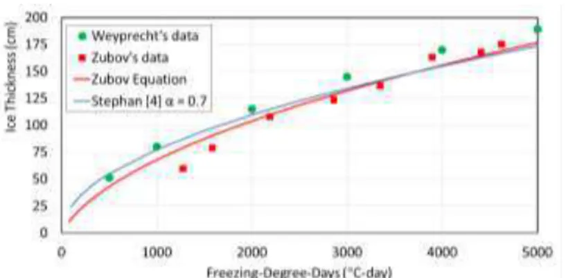
Sea ice growth in Arctic regions occurs under different conditions due to the high latitude; limited solar radiation during the principle growth period. Zubov (1945), made extensive measurements of ice thickness and climate in the Russian Arctic. Using his own measurements and noting those of Weyprecht (1879), also made in the Arctic, he proposed an empirical expression for predicting sea ice thickness
h2 + 50h = 8 S [5]
In Zubov’s equation S is in units ºC-day and ice thickness h, cm. Zubov’s and Weyprecht’s data, together with Zubov’s equation [5], and a modification of Stefan [4] with α = 0.7 are plotted in Figure 1. The Zubov equation [5] is a good fit to the data. The Stefan equation, adjusted by applying a local conditions coefficient, α = 0.7, provides a reasonable comparison to the data, but it tended to over-predict for thin ice and under-predict for thick ice.
While much focus has been on the ice properties and coefficients that go into equation [4], the accumulated freezing-degree-day term, S, also bears attention. Note: freezing-degree-day will be abbreviated f-d-d hereafter. Establishing the start for the accumulation of f-d-d is a question. In this paper the start is the day after which the accumulated f-d-d, as defined by S in equation [3] is consistently negative. At some locations the water may still be cooling at this time. Where it is available, counting from freeze-up is more representative. This is a more critical issue when predicting ice thickness during the early part of the winter than the maximum ice thickness. Other investigators have looked into developing improved practical equations for predicting ice thickness from general environmental conditions. Sinha and Nakawo (1981) used detailed high-quality ice, snow and climatological measurements from Eclipse Sound in the Canadian High Arctic, to develop and test an ice thickness prediction model suitable for the conditions of the high Arctic. The equation developed was similar in form to Zubov’s
h2 + 2 (ki / ks) hs h = 2 (ki / λ ρ) S [6]
They had frequent measurements of ice thickness, salinity, temperature profiles, snow thickness and density, as well as daily air temperatures. Using mean annual snow thickness and density, plus properties of sea ice from the literature, equation [6] made good predictions of ice thickness throughout the two winters for which they had data to test it. Note, that care always has to be paid to consistent units on both sides of the equation.
The draft of the new edition of ISO 19906 Arctic offshore structures (ISO, 2017) has an equation for predicting sea ice growth
h2− ho2 + m (h − ho) = ω S [7]
where h is the current ice thickness, ho an initial ice thickness, and S in this case is the
accumulated f-d-d between when ho was determined and the time when the current ice thickness
h is to be determined. The physical parameters of equation [7] are defined as m = 2 (ki / ks) hs and
ω = β 2 ki / λ ρ, essentially the same as in equation [6]. The only exception is the introduction of
β, an empirical factor introduced to take into account local conditions, but not necessarily the
same as α in equation [4]. If ho is set to 0 it is seen that the ISO equation [7] is identical to the
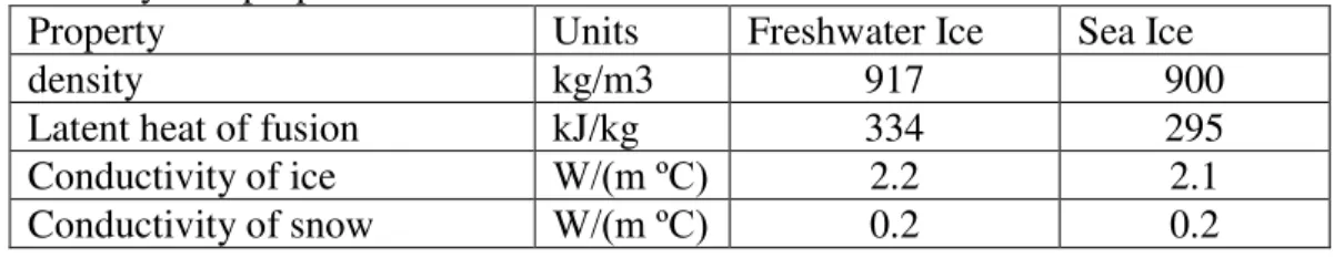
Sinha and Nakawo (1981) equation [6]. Some typical values of ice and snow physical properties are listed in Table 1. It should be noted these properties are all temperature and salinity dependent, some to a greater extent than others. For example, the latent heat of fusion of sea ice is quite dependent on its temperature and salinity. Similarly the conductivity of snow is very dependent on its density. Weeks (2010) provides a good review of snow and sea ice properties, including their temperature, salinity and density dependence.
Table 1. Physical properties of ice and snow.
Property Units Freshwater Ice Sea Ice
density kg/m3 917 900
Latent heat of fusion kJ/kg 334 295 Conductivity of ice W/(m ºC) 2.2 2.1 Conductivity of snow W/(m ºC) 0.2 0.2
3. Examples of ice growth
There are 10 weather stations in the Canadian Arctic at which ice thickness and snow depths are systematically measured throughout the winter, plus the usual meteorological data. The predictive capability of equations [4] and [7] were tested against some of these measured data. Two stations have been selected for this purpose; Resolute (72º 42’ - N 94º 50’ W) where measurements are made in sea ice and Baker Lake (64º 19’ - N 96º 01’ W) in fresh water ice. At Resolute Bay measurements extend back to the late 1940s. The approach is to use f-d-d determined from air temperature measurements at the locations with properties for sea ice and freshwater ice from Table 1 to calculate an ice thickness. It will also be investigated how snow depth information can be used to improve the prediction of ice thickness.
Resolute Bay, Nunavut, Canada: Measured and predicted ice thicknesses together with snow depth for the winter 2005-06 is plotted in Figure 2. The α and β factors, noted on the figure, were adjusted to match the maximum ice thickness. The basic parameters and factors for the winter of 2005-06 and 2006-07 are summarized in Table 2. The winter 2005-06 had fewer f-d-d (8% less) than 2006-07, a greater snow depth (100% more), and not surprisingly, a lesser maximum ice thickness (12%). Based on f-d-d alone, the thickness should have been only about 4 % less. It is clear that the snow depth has a strong influence. The modified Stefan equation [4] has no direct means of incorporating snow depth, other than local conditions coefficient α. On the other hand, the ISO equation [7] has the possibility of including both the snow depth and, if known, the snow conductivity, while still providing some facility for local conditions with the factor β on the
accumulated f-d-d term, S. It appears that with α of 0.75, equation [4] could have utility. The variability of β for just these two winters’ factor brings into question the utility of equation [8].
Table 2. Ice growth parameters at Resolute Bay for winters of 2005-06 and 2006-07
Winter FDD Max Ice thickness (m) Mean snow depth (m) α factors β factor
2005-06 4630 184 0.22 0.75 1.9
2006-07 4990 210 0.11 0.77 1.3
Next the entire Resolute Bay record in terms of maximum annual ice thickness, mean annual snow depth and accumulated f-d-d is plotted in Figure 3 to illustrate year-to-year variation. Maximum annual ice thickness was examined in reference to accumulated f-d-d, S, and mean annual snow depth, hs, and their influence shown by plotting them versus the measured
maximum annual ice thickness in Figure 4. A stronger correlation to snow depth than f-d-d was seen. Some other Canadian Arctic station records were checked and generally similar relative influences were found. Based on this, a modified form of equation [7] was developed by inserting an empirical coefficient, γ, into the m term, since this is where snow depth comes into play. Thus a modified ISO equation was proposed
h2− ho2 + γ m (h − ho) = ω S [8]
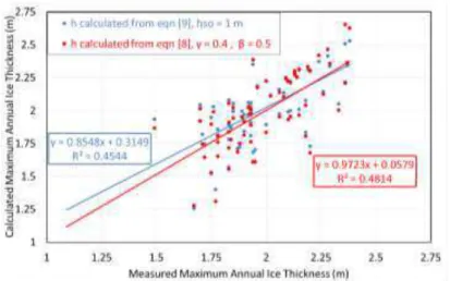
with the empirical coefficient β set to 0.5. Based on the observed influence of snow depth, a modified equation [4] with a factor to include the influence of snow depth was also developed as
h = 0.037 (1-hs/hso) S1/2 [9]
where hso is a normalizing snow depth selected to non-dimensionalize the snow depth, in this
case hso = 1 m. The results of the calculated maximum annual ice thickness using equations [8]
and [9] are plotted in Figure 5. The predictions of the two equations are similar, with [8] coming closer to one to one slope on the linear regression than equation [9].
Baker Lake, Nunavut, Canada: The entire Baker Lake record in terms of maximum annual ice thickness, mean annual snow depth and annual accumulated f-d-d is plotted in Figure 6 to illustrate year-to-year variation. This site is a freshwater lake about 300 km inland from Hudson Bay, and has significantly less snow. Baker Lake has a slightly less severe winter with about 4500 °C-day versus about 5500 °C-day for Resolute Bay. Maximum annual ice thickness attained at Resolute Bay is less than at Baker Lake due to the difference in snow depth.
The relation between mean annual snow depth and f-d-d was examined versus maximum annual ice thickness. For snow depth a slight trend of increasing ice thickness with decreasing snow depth could be ascertained, but it was not significant. The relation to f-d-d was more pronounced. Calculated maximum annual ice thickness for all three prediction equations, [4], [8] and [9] are plotted in Figure 7. For the case of Baker Lake conditions the simple Stefan equation with α = 0.9 provided the best prediction within the limited range of maximum annual f-d-d associated with this location. The parameters in equations [8] and [9] were adjusted to see if a
better fit could be obtained, but the ones displayed on Figure 7 were the best that could be determined.
4. Summary and Conclusions
In the Canadian High Arctic, the amount of snow is a significant factor, in addition to winter severity (accumulated freezing degree days), in determining the maximum annual ice thickness in marine environments. Marine coastal sites in the Arctic generally have more snow than inland sites and consequently thinner ice, given comparable winter severity. The modified equations in this paper, [8] and [9], provide better utility for predicting maximum annual sea ice thickness by including weighing functions for snow thickness. Equation [8], with two local conditions factors should be useful for predicting ice thickness during the growth period. Future effects of climate change, including snowfall, on ice thickness can be evaluated with the aid of these equations. For engineering design purposes any apparent trends in ice thickness should also take into account the large annual variability, which is evident in the actual records and would likely persist or even increase in the future.
Acknowledgments
The support of the Arctic Program of the National Research Council is gratefully acknowledged
References
Ashton, G.D. 2011. River and lake ice thickening, thinning, and snow ice formation, Cold Regions Science and Technology, Vol. 68, pp. 3–19
ISO. 2017. ISO/FDIS 19906 Arctic offshore structures, International Organization for Standardization, Geneva
Leppäranta, M. 1993. A review of analytical models of sea ice growth, Atmosphere-ocean, Vol. 31, pp.123-138
Michel, B. 1971. Winter regime of rivers and lakes, Cold Regions Science and Engineering Monograph III-B1a. CRREL, Hanover, NH. April 139 pp.
Sinha, N.K. and Nakawo. M. 1981. Growth of first-year sea ice, Eclipse Sound Baffin Island, Canada, Canadian Geotechnical Journal, Vol. 18, pp. 17-23.
Stefan, J. 1891. Uber die Theorie der Eisbildung, insbesondere uber die Eisbildung im Polarmeere, Annalen der Physik und Chemie, 42, pp. 269-286.
Wayprecht, K. 1879. "Die Metamorphosen des Polareises" (The metamorphoses of polar Ice), Austro-Hungarian Arctic Expedition of 1872-74, 1879.
Weeks, W.F. 2010. On Sea Ice, University of Alaska Press, Fairbanks
Zubov. N.N. 1945. L’dy Arktiki [Arctic Ice]. Izdatel’stvo Glavsermorputi, Moscow. English Translation. 1963 by U.S. Naval Oceanographic Office and American Meteorological Society, San Diego, Calif.
Fig. 1. Ice thickness as a function of freezing-degree-days from data and Zubov’s equation.
Fig. 2. Comparison of measured and predicted ice growth at Resolute Bay
Fig. 3. Resolute Bay record of ice thickness, snow depth and freezing-degree-days
Fig. 5. Predictions of maximum annual ice thicknesses for Resolute Bay
Fig. 6. Baker Lake record of ice thickness, snow depth and freezing-degree-days
![[PDF] Formation général pour débuter avec le CMS Drupal | Cours informatique](data:image/gif;base64,R0lGODlhAQABAIAAAP///wAAACH5BAEAAAAALAAAAAABAAEAAAICRAEAOw==)