N
UEAR
MITNE-251 APPLICATION OF
TIME DEPENDENT UNAVAILABILITY ANALYSIS TO STANDBY SAFETY SYSTEMS
Andrew Arthur Dykes
Massachusetts Institute of Technology Norman C. Rasmussen
Massachusetts Institute of Technology William E. Vesely, Jr.
Battelle Memorial Institute
MASSACHUSETTS INSTITUTE OF TECHNOLOGY
Department of Nuclear Engineering Cambridge, Massachusetts 02139
June 1982
Prepared for Brookhaven National Laboratory under Contract No. BNL-546681
NOTICE
This report was prepared as an account of work sponsored by the United States Government. Neither the United
States nor the United States Nuclear Regulatory Commission, nor any of their employees, makes any warranty, express or implied, nor assumes any legal liability or
responsib-ility for the accuracy, completeness or usefulness of any information, apparatus, product or process disclosed, nor represents that its use would not infringe privately owned rights.
0
APPLICATION OF
TIME DEPENDENT UNAVAILABILITY ANALYSIS TO STANDBY SAFETY SYSTEMS
by
ANDREW ARTHUR DYKES
Submitted to the Department of Nuclear Engineering on May 19, 1982 in Partial Fulfillment of the
Requirements for the Degree of Doctorate in Philosophy ABSTRACT
The FRANTIC II computer code has been modified and used to demonstrate that time dependent unavailability analysis is a practical tool for assessing the periodic testing programs of operational standby safety systems.
FRANTIC II was assessed from an engineering point of view and modified as necessary to make it more useful for appli-cation to operational systems. An offset time was. added to the component failure parameters to provide more flexible
modeling of time dependent standby failures and the effects of test caused wear-out. A routine to calculate the optimum test interval of a constant failure rate component subject imperfect testing was also developed. The code was then coupled to a cutset generator and evaluator for application
to multiple component systems. The resulting code is named FRANTIC II-MIT.
FRANTIC II-MIT has been applied to the High Pressure Coolant Injection System of a Boiling Water Reactor and a
quantitatively based periodic testing program keyed to a fault tree evaluation of the system' s safety functions has been formulated. The analysis indicated that system una-vailability can be reduced while also reducing testing
requirements from approximately 170 to 123 tests per year.
-Thesis Supervisor: . Norman C. Rasmussen
Title: Professor of Nuclear Engineering Thesis Supervisor: William E. Vesely, Jr.
TABLE OF CONTENTS
Chapter 1 INTRODUCTION .
1.1 Background and Motivation 1.2 Purpose and Scope . . . 1.3 Structure of Thesis . . .
Chapter 2 UNAVAILABILITY AND PERIODIC TESTING 2.1 Standby System Unreliability Definitions
Unavailability, Q(t1 ). . ... Cumulative Failure Probability, P(tilt2)
Unreliability, F(t1,t ) . . . . . . . . . . . 2.2 Basic Unavailability Concepts . . . . . .
2.2.1 "Other" Components . . . . . 2.2.2 Periodically Tested Components . . . . 2.3 Current Status of Analysis of Periodic Tes
2.3.1 Regulations and Standards . . . . . . .
2.3.2 Published Reseach. . ...
Simple Systems With Test Downtime . . . . .
Redundant Standby Components . . . . . . . . Effects of Human Error on Simple Systems Components With Many Failure Mechanisms 2.,3.3 Application to Fault Tree Analysis 2.3.4 The FRANTIC II Computer Code
13 13 14 . . . . . 15 17 18 18 22 ting . . . 25 . . . . 26 29 29 36 40 47 55 57 iv . . . . . .1 . . . . . . 3 . . . . . 7 . . . .10
TABLE OF CONTENTS (Continued)
Chapter 3 ENGINEERING INTERPRETATION OF FRANTIC II-MIT 3.1 Overall Structure . . . . 3.1.1 Unavailability Equations . . . . . . . . . . 3.1.2 Calculation Procedure .. . . ... . . .. . . 3.2 Standby Failure Rate . . . . . . . . . .
3.2.1 Scale Factor for Detectable Standby Failures . 3.2.2 Scale Factor for Undetectable Standby Failures
3.2.3 Failure Rate Shape Factor . . . o.. ... .. 3.2.4 Component Renewal Type . . . . . . . .
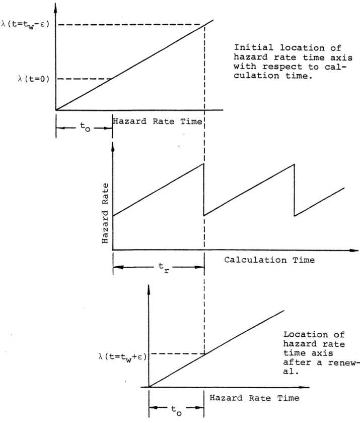
Use of Offset Time With Renewal Types . . . 3.2.5 Test Caused Changes to Scale Factor . . 3.2.6 Unavailability Due to Standby Failures
Monitored Components
Periodically Tested Components . . . . . . . 3.3 Demand Failure Rate . . . . . . . . . . .
3.3.1 Engineering Interpretation . . . . . . 3.3.2 Special Uses . . . . . . . . . . . . . 76 78 78 79 79 . . 80 82 . . . . 82 . . 83
Monitored Failures in Periodically Tested Components Common Cause Failures . . . . . . . . . . . . . . .
3.4 Times Associated with Periodic Testing . . . . . .
3.4.1 Periodic Inspection Interval . . . . . . . . .
3.4.2 First Periodic Inspection Interval . . . . . .
3.4.3 Scheduled Test and Maintenance Period... 3.4.4 Unscheduled Repair Time . . . . . . . . . . . .
. . 60 . . 62 62 65 . . 71 73 . . 74 75 . . 83 84 84 . 85 85 85 86
TABLE OF CONTENTS (Continued)
3.5 Effects of Imperfect Testing . . . . . . . . . . . 87
3.5.1 Probability of Test Caused Failure . . .. ... 87
3.5.2 Unavailability to Override Test and Maintenance 88 3.5.3 Test Caused Failure Rate Change Factors . . . 89
3.5.4 Test Error Carryover Factor . . . . . . . . . 92
3.6 Generalized Weibull Hazard Rate . . . . . . . . . 93
3.6.1 Susceptibility of Component Failure Mechancisms 95 3.6.2 Effects of Offset Time on Hazard Rate . . . . 98
3.6.3 Advantages Over FRANTIC II Hazard Rate . . . . 102
3.6.4 Estimating Input Parameters . . . . . . . . . 109
3.6.5 Alternate Models of Time Dependency ... 114
Chapter 4 APPLICATION TO SINGLE COMPONENT SYSTEMS . . . 118
4.1 Demand Verses Standby Failures . . . . . . . . . . 118
4.1.1 Ratio of Observed Demand and Standby Failures . 119 Beta = 1 Standby Failure Rate . . . . . . . . . . . . 121
Beta = 2 Standby Failure Rate, NN Renewal . . . . . . 123
4.1.2 Effect of Increasing Demand Failure Rate . . . 126
4.1.3 Effect of Undetectable Failures . . . . . . . . 126
4.1.4 FRANTIC Code Assumption Regarding Demand Failures . . . . . . . . . . . . . . . . . . . . . . 129
4.2 Subroutine OPTEST . . . . . . . . . . . . . . . . . 130
4.2.1 Background . . . . . . . . . . . . . . . . . . 130
4.2.2 Theory . . . . 130 vi
TABLE OF CONTENTS (Continued)
4.2.3 Implementation in FRANTIC II-MIT. ... 4.2.4 Comparison With FRANTIC II-MIT RUN Option
4.3 Behavior of Constant Failure Rate Components . . . .
4.3.1 Approximate Relative Importance of Failure Modes 4.3.2 Effective Test Downtime .
4.3.3 Unavailability Contours . . . . .
4.4 Behavior of Time Dependent Hazard Rate 4.4.1 Importance of Hazard Rate .
4.4.2 Uses of Renewal Options
New-New Renewal .... ... Old-New Renewal . . . . . . . . . . . . Old-Old Renewal . . . . . . . . . . . . 4.5 Test Caused Wear-Out and Burn-In .
4.5.1 Effect on Standby Failure Rate 4.5.2 Effect on Demand Failure Rate
4.6 Summary . . . . . . . . . . . . . . . Components 145 . 147 149 . . . ... ... .149 ... ... 151 ... ... 151 ... ... 152 ... ... 153 ... ... 157 ... ... 157 ... ... 161 ... ... 161
Chapter 5 APPLICATION TO MULTIPLE COMPONENT SYSTEMS 5.1 CUTSETS . . . . . . . . . . . . . . . . . . . . 5.2 Some Applications to Simple Systems . . . . . . 5.2.1 Series Systems . . . . . . . . . . . . . . . 5.2.2 Demand Failures and Redundant Components . . 5.2.3 Effect of Unequal Test Override . . . . . . . . . 163 . . . 164 . . 170 . . . 170 172 174 . 138 . 139 . 143 . 143
TABLE OF CONTENTS (Continued)
5.3 Comparison With Vaurio's l-out-of-3 System
Calculation . . . 174
System Description and Cut Sets ... ... 176
5.4 An Approach for Analyzing Systems . . . . . . . . . 183
Chapter 6 APPLICATION TO A HIGH PRESSURE COOLANT INJECTION SYSTEM . . . 186
6.1 Introduction . . . . . . . . . . . . . . . . . . . . 186
Organization of Analysis . . . 187
6.2 Description of System Functions . . . . . . . . . , 189
6.2.1 Safety Functions .... . .. .. .. .. .. 190
6.2.2 Injection Function . . . . . . . . . . . .... 192
Actions Required for Injection . . . . . . . . . . . 192
6.2.3 Autoisolation and Termination . . . . . . . . . 195
Actions Required for Autoisolation . . . . . . . . . 198
6.3 Fault Tree Analysis ... .. ... 198
6.3.1 Assumptions . . . . . . . . . . . . ... . . . . 199
6.3.2 Qualitative Analysis . . . . . . . . . . . . . . 201
6.3.3 Quantitative Analysis . . . . . . . . . . . . . 205
6.4 Turbine/Pump Train Operability Tests . . . . . . . . 205
6.4.1 Description of Online Tests . . . . . . . . . . 205
Recommendations for Consolidation . . ... 207
6.4.2 Description of Operating Cycle Tests . . . . 207 .
TABLE OF CONTENTS (Continued)
6.4.3 Quantitative Analysis of Operational Tests Super Component Failure Rate . . .
Steam Supply Valve Failure Rate
Unavailability During Testing . . .
Results . . . . . . . . .
Recommendations . . . . . . . . . . 6.5 Automatic Initiation Function Tests
6.5.1 Initiation Sensor Tests . . . .
Quantitative Analysis . . . . . . . 6.5.2 Description of Initiation Logic Current Test Policy . . . . . . . .
Comments on Current Test Procedures
6.5.3 Quantitative Evaluation of Initiation Unavailability Using Current Logic Design
Initiation Logic Relay Modifications . . .
Summary and Recommendations . . . . . . .
6.6 Autoisolation Function Tests . . . . . .
6.6.1 Quantitative Analysis . . . . . . . . Common Cause Effects
Important Cut Sets
Interaction With Injection Function .
Recommendations . . . . . . . . . . . . .
6.7 Summary of HPCI Recommendations . . . . .
. . . . 209 . . . . 212 . . . . 215 . . . 217 . . . . . 227 . . . . 227 . . . . 231 . . . . 232 Tests . . . . . .. 237 .237 .238 Logic Tests . 239 . 241 . 244 . . . . 248 . . . . . 250 .255 .255 .256 .260 .263 . . . . . . 266 . .
TABLE OF CONTENTS CContinued)
Chapter 7 SUMMARY, CONCLUSIONS AND RECOMMENDATIONS . 273 7.1 Summary ... .... ... 273 7.2 Conclusions . . . . . . . 275 7.3 Recommendation for Further Research . . . . . . . 277
APPENDICES
A HPCI Injection Function Fault Tree
B HPCI Injection Function Cut Sets . . . . . . C HPCI Injection Function Components . . . . . D HPCI Injection Function Fault Tree
Modifica-tions Resulting From Initiation Logic Changes E HPCI Initiation Function Cut Sets (Before
and After)
F HPCI Autoisolation Function Fault Tree . G HPCI Autoisolation Function Cut Sets . . .
H HPCI Autoisolation Function Components . . .
I FRANTIC-II Input
J The CUTSETS Package . . . . . . . . . . . . . K Running FRANTIC II-MIT on-CMS . . . . . . . .
. 285 . 305 . 312 . 316 . 319 . 324 . 332 . 335 . 337 . 355 . 360
(
xList of Figures
Figure Description
1.1 Simplified Example of a Periodically Tested 4 System.
2.1 Time Dependent Unavailability of Components 19 Other Than Those That Must Be Periodically
Tested to Reveal Standby Failures.
2.2 Time Dependent Unavailability of Components 23 Which Must Be Tested to Reveal Standby
Failures.
2.3 Example of the Effect of Test Interval on Com- 30 ponent Unavailbility When the Component is
Com-pletely Unavailable for its Safety Function While Being Tested.
2.4 Unavailability of a Component Subject to Stand- 30
by Failures and Test Downtime. [Ja68I
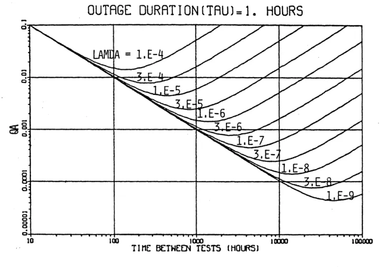
2.5 Average Component Unavailability Verses Time 35
Between Tests, Parametric With Component Fail-ure Rate, X (failFail-ures/hr), Outage Duration (r)
= 1 hour. (Figure 4 of NUREG/CR-2158)
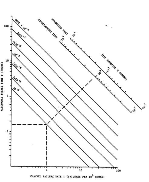
2.6 Nomograph for Calculating a Test Interval and 39
Duration to Meet an Unavailability Goal. Exam-ple for 2-out-of-3:Good Logic. [Hi7l]
2.7 Optimal (Maximum Availability) Test Interval 42
and Associated Availability as a Function of
pA*. [McW80]
2.8 Optimal (Maximum Availability) Test Interval 42
and Associated Availability as a Function of
pB. [McW80]
-2.9 Test Interval of Diesel Generator Failures. 49
[Ma82]
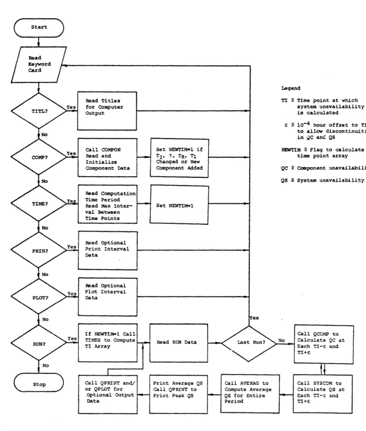
3 . 1 Computational Flow of the FRANTIC Computer Pro- 66
grams.
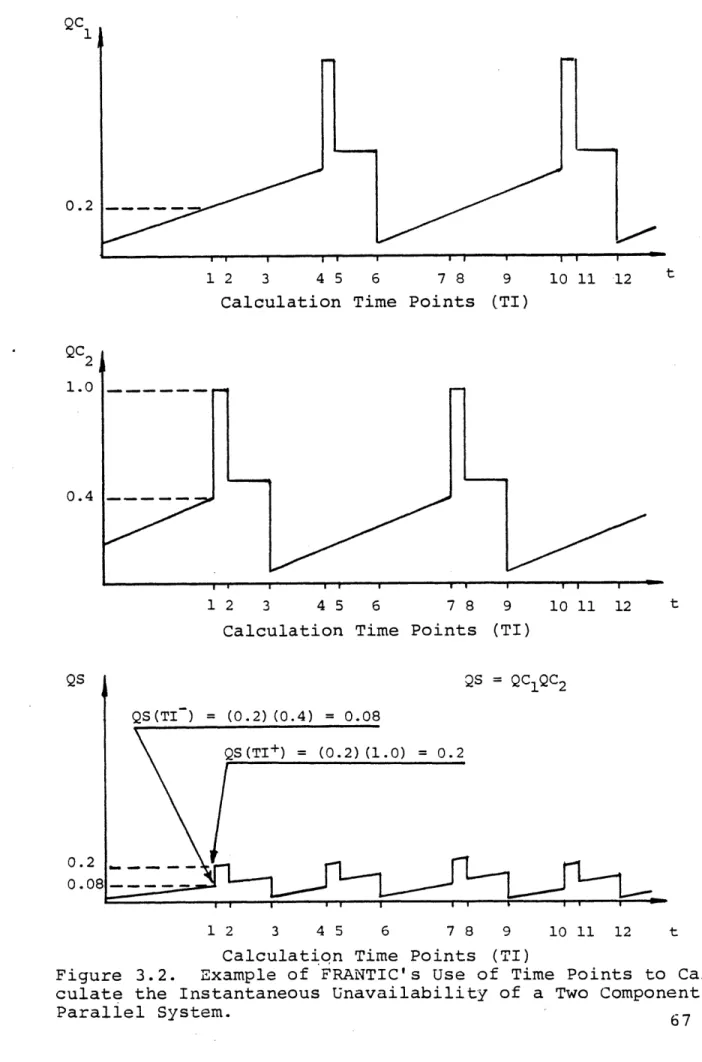
3.2 Example of FRANTIC's Use of Time Points to Cal- 67 culate the Instantaneous Unavailability of a
List of Figures
Figure Description
3.3 FRANTIC II-MIT Output of System Unavailiblity 70 Data Resulting From a Calculation Using the Run
Option.
3.4 Use of Offset Time and Renewal Options to 100 Obtain Time Dependent Failure Rates With a
Gen-eralized Weibull Hazard Rate.
3.5 Five Failure Rates Modeled With a Two Parameter 104 Weibull Hazard Rate Which Rise From 0 at Time
Zero to 1.0xE-5/hr at 20 Years.
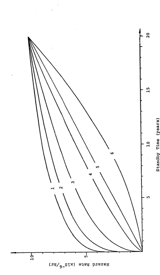
3.6 Five Failure Rates Modeled With a Generalized 108 Weibull Hazard Rate Which Rise From 1.OE-6/hr
at Time Zero to 1.OE-5/hr at 20 Years.
3.7 Normalized Weibull Hazard Rate. 110 3.8 Use of the Normalized Weibull Hazard Rate 112
Curves to Obtain Offset Time.
3.9 Failure Rates for Selected Values of 5, X, and 115 t which start at the same initial value.
3.10 Use of an OR Gate to Obtain a Failure Rate Time 117 Dependence Which Does Not Follow a Power Law.
4.1 Sensitivity of Component Unavailability to 120
Demand Verses Standby Failure Mechanisms, Con-stant Standby Failure Rate, Downtime per Test =
1 Hour.
4.2 Sensitivity of Component Unavailability to 124
Demand Verses Standby Failure Mechanisms, Beta = 2 Standby Failure Rate, Downtime per Test = 1
Hour.
4.3 Effect of Periodic Testing on a Component With 127
a Constant Standby Failure Rate and Various
Magnitudes of Demand Failure Rate.
4.4 Graphical Representation of the Time Inte- 131
grated Unavailability of a Periodically Tested
Component.
4.5 Comparison of OPTEST and RUN Calculations of 140
the Average Unavailability of a Periodically Tested Component Verses Test Interval.
List of Figures
Figure Description
4.6 Average Unavailability Contours for a Period- 148 ically Tested Component Having an Effective
Downtime per Test of One Hour.
4.7 Instantaneous Unavailability Resulting From 150 Hazard Rates Having Three Different Time
Dependencies.
4.8 Effect of Variations in the Maintenance Inter- 156 val on a Time Dependent Hazard Rate.
4.9 Long Term Effect of Test Caused Wear-out in 159
Standby Failure Mechanisms. Example for f =
1.01.
5.1 Cut Set Generator Flow Chart. [Ka80] 165 5.2 Equivalent Transformation of EOR, NAND, NOR, 168
and NOT Gates. [Ka80]
5.3 Effect of Demand Failure Mechanisms on the 173 Optimum Test Interval of a Parallel Component
System.
5.4 Comparison of Testing Policies for Parallel 175 Components with Unequal Unavailabilities
Dur-ing the Test Period.
5.5 Single Line Diagram of the 1-out-of-3, Two 177
Valve per Redundancy, Test System Used in the Comparison Between FRANTIC and ICARUS.
5.6 Fault Tree of the 1-out-of-3, Two Valve per 179 Redundancy, Test System.
6.1 Simplified Diagram of the High Pressure Coolant 191 Injection System of a Boiling Water Reactor.
6.2 Optimum Test Interval of HPCI Turbine/Pump as a 218
Function of Composite Failure Rate and
Effec-tive Downtime Per Test.
6.3 Average Unavailability Contours for HPCI Tur- 220
bine/Pump Testing When Effective Downtime per Test is One Hour.
6.4 Average Unavailability Contours for HPCI Tur- 221
bine/Pump Testing When Effective Downtime per Test is Two Hours.
List of Figures
Figure Description
6.5 Average Unavailability Contours for HPCI Tur- 222 bine/Pump Testing When Effective Downtime per
Test is Three Hours.
6.6 Average Unavailability Contours for HPCI Tur- 223 bine/Pump Testing When Effective Downtime per
Test is Four Hours.
6.7 Super Component Unavailability Verses Test 224 Interval for the Various Combinations of Demand
and Standby Failure Rates Given in Table 6.3.
6.8 Effect of Test Caused Wearout on Optimum Test 226
Interval.
6.9 Simplified Diagram of HPCI Initiation Function 228 Components.
6.10 Initiation Logic Signal Flow. 229
6.11 Average Unavailability of Initiation Sensors 233 Without Common Cause Failures.
6.12 Average Unavailability of Initiation Sensors 235 With Common Cause Failures Within Individual
Groups of Sensors.
6.13 Average Unavailability Due to Online Testing of 240 the Initiation Logic Relays.
6.14 Unavailability of Initiation Logic Relays. 243
With Current Design and Current Test Procedures and Staggering.
6.15 Wiring Diagram of HPCI Initiation Logic with 246
Modifications 2 and 3.
6.16 Changes in Relay Logic Signal Flow Produced by 247 Modification Two.
6.17 Effects of Design Modifications on Initiation 249 Function Unavailability Verses Periodic Test
Interval. Effective Downtime per Test = 2.0
hours.
6.18 Sensitivity of Modified Initiation Logic Cir- 251 cuit Unavailability to an Order of Magnitude
Increase in Component Failure Rates.
List of Figures
Figure Description
6.19 Autoisolation Function Unavailability as a 258 Function of Autoisolation Sensor Test
Inter-vals.
6.20 Injection Function Unavailability Due to 264 Autoisolation Sensor Tests Which Cycle
List of Tables
Table Description
2.1 Table 4 of ANSI/IEEE Standard 352-1975. Test 28 Interval as a Function of Logic Configuration
and Unavailability Design Goal G.
2.2 Component Unavailability Equations for Four 37 Classes of Components. [Ca77]
3.1 Parameters Used for Plotting Curves in Figure 103 3.5.
3.2 Values of , X , and t Used to Obtain the Hazard 107 Rate Curves Shown in Figure 3.6.
4.1 Component Failure Parameters for Figures 4.1 122 and 4.2 and Plots of the Resultant Hazard Rates
as a Function of Time.
4.2 Input and Output of OPTEST Calculations for 141 Figure 4.5.
4.3 Input and Output of RUN Calculations for Figure 143 4.5.
4.4 Comparison of Calculations Using the Old-Old 154 Renewal Option and a S=3 Hazard Rate With Those
Using an Equivalent Constant Failure Rate.
5.1 Input and Output of CUTSETS Application to the 180
Test System.
5.2 Input Parameters for the 1-out-of-3, Two Valves 181
Per Redundancy, Test System.
5.3 Input of FRANTIC II-MIT Application to the Test 181
System.
5.4 Results of Comparison of Uncorrected and Cor- 182
rected Versions of FRANTIC with Vaurio's
Calcu-lations.
6.1 HPCI Injection Function Single Component Cut 202 Sets.
6.2 Assessed Range of Single Component Cut Sets 211
Tested by the HPCI Turbine/Pump Test.
6.3 Range of Super Component Failure Rates for Tur- 212 bine/Pump Test.
List of Tables
Table Description
6.4 Upper Bound Estimates of MO 2301-3 Standby 213 Failure Rate Since 1975.
6.5 Probability of Test Caused Failure to Injection 263 Function Failure Events 31 and 32 (Isolation
Valves, NOFC) as a Result of Autoisolation Function Tests.
CHAPTER 1 INTRODUCTION
Standby safety systems have the very difficult mission of remaining idle for long periods of time while being pre-pared to function under accident conditions at a moment's
notice. The operational status of most of these systems can not be monitored while they are idle, so the Nuclear Regula-tory Commission (NRC) requires that systems important to safety "be designed to permit appropriate periodic
inspection of important areas and features. . . " [ 10CFR50,
App. A] Unfortunately, establishing a quantitative basis
for judging what is appropriate is very difficult for a com-plex saftey system containing many components. As a result, periodic test and inspection policies are frequently based on "engineering judgment" or the anaylsis of equivalent
sin-gle component systems, rather than a quantitative balancing of the advantages and disadvantages of accomplishing a par-ticular testing program in the context of the entire
system's safety function.
To aid in establishing a more quantitative basis for periodic testing, the NRC has developed and distributed the FRANTIC (Formal Reliability Analysis including Normal Test-ing, Inspection and Checking) computer codes. [Ve77,
Ve81] The codes use time dependent unavailability
sis to accomplish this task. Given a comprehensive set of input parameters describing component failure rates and periodic testing policies and a user supplied equation relating the system's unavailability to that of the compo-nents, they calculate the system's instantaneous unavail-ability at all important time points and the average system unavailability over a user specified calculation period. Two versions are currently available. The original FRANTIC code assumes constant component failure rates, while FRAN-TIC II can model wear-out and burn-in as a function of both calendar time and periodic tests. While the codes have been
applied to illustrative examples (eg. EP1443, Va79b, Ka80], to the best of this author's knowledge, they have not yet been used for a detailed examination of the periodic testing program for an operating reactor system.
The purpose of this thesis is to assess the utility of time dependent unavailability analysis for improving the availability of standby safety systems using the FRANTIC II computer code as a tool. To accomplish this, FRANTIC II is assessed from an engineering point of view and modified as necessary to make it more useful for applications to opera-tional systems. It is then interfaced with a cutset
generator and evaluator so that is can be applied to complex system models. The modified verison of the code is named FRANTIC II-MIT. The code is then applied to the High
and a quantitatively based periodic testing policy keyed to a fault tree evaluation of the system's safety functions is established. As a result, this thesis provides an improved framework within which a systems engineer can establish a quantitative basis for a periodic testing program.
1.1 BACKGROUND AND MOTIVATION
To illustrate the primary motivation for accomplishing periodic testing, consider the following simple example. Figure 1.1 represents the time dependent unavailability of a
standby safety system whose failure rate can be modeled by a single constant standby failure rate, Xs per hour, and which can be tested in its entirety at one time. This parameter models the system's suseptibility to random shocks that transfer it into a state which can not respond to a demand to
operate. [Ba75, Ap76, EP14431 However, because the system is idle, the shocks do not produce observable effects until the demand is actually made. As the system sits idle, the
time during which the shocks can occur lengthens and the
probability that a failure has occurred gradually
increases. When a test is accomplished, the demand to oper-ate is made and the failures are revealed and immediately
repaired. After the test the system' s unavailability is zero because random shocks have not yet had an opportunity to occur.
Periodic Test
r-Standby Time
Figure 1.1. Simplified Example of a Periodically Tested System
In practice, standby failures are not the only factor to consider in establishing a periodic test policy. For example:
* Shocks may occur during the demand as well as during the standby period. They produce failures whose probability is independent of the standby period. If demand related failures are possible, the unavailability of a component is not reduced to zero by an operational test.
e Frequently a system must be reconfigured to test an
acci-dent mitigation function without interfering with normal operations, and it may be unavailable to perform that
function in the event that a true demand occurs during the test.
* Operational tests which cycle the system to an active mode may cause wear-out that makes the system more suseptable
to failures later in its life.
* Since test conditions are not always similar to accident conditions, a periodic test may not be able to detect all the failure mechanisms which could prevent the system from performing its intended function.
* The act of accomplishing the test can cause failures which require repair and thus produce additonal unavailability.
* Human error during the test may leave the system in a failed state at its conclusion.
Clearly, there are positive and negative aspects of periodic testing which must be balanced when formulating a periodic testing program.
Even if one accounts for all the factors mentioned in the previous paragraph, a simple one component system fre-quently can not be used to model operational systems. Engi-neered safeguards systems in a nuclear reactor are a prime example. They contain many components which exhibit a vari-ety of failure mechanisms. Within the context of these
complex systems, all the considerations listed for the sim-ple system of the previous paragraph now apply to each
component. It is difficult to establish an optimal testing policy for these systems for several reasons:
* Direct testing of the entire safety function usually can not be performed without interfering with the operation of the reactor, so portions of the system must be recon-figured, disabled or bypassed, while other parts come into closer alignment with their operational configura-tion
* The system is frequently designed to respond to diverse indications of an accident, each of which must be tested
separately.
* The act of testing some components can affect the status of both the component being tested and other groups of
* Testing of individual components can cause failures which must be repaired. Frequently the entire system is
disa-bled during the repair.
Until recently, a reasonable tool for establishing a quantitative basis for a periodic testing program which
con-siders all of the above factors did not exist. It is very difficult to evaluate the effect of individual component failure mechanisms on the functioning of a larger system having many different types of components without a tool
such as a computer code to reduce the computational diffi-culties. The Nuclear Regulatory Commission has recently developed the FRANTIC II computer code to alleviate this problem. The code calculates component unavailability at specific points in time taking into account both demand and time dependent failure rates and modeling both the positive and negative effects of periodic testing. A user provided equation is then called to calculate the system
unavailabil-ity in terms of individual component unavailibilities.
Because it has not yet been applied to actual system
prob-lems, FRANTIC II's capabilites and limitations have not yet
been explored.
1.2 PURPOSE AND SCOPE
The purpose of this thesis is to assess the usefulness of time dependent unavailability analysis for improving the availability of standby safety systems using the FRANTIC II
computer code as a tool. To accomplish this goal, the fol-lowing tasks are performed:
1) Modification of FRANTIC II as necessary to provide modeling capability of physically reasonable failure mech-anisms. The resulting code is named FRANTIC II-MIT. The task includes:
* An engineering interpretation of failure mechanisms of standby components subject to periodic testing and repair.
* Correlation of FRANTIC II input parameters with these mechanisms
* Incorporation of an additional model which accounts for test caused changes in the demand failure rate.
* Incorporation of an offset time into the Weibull hazard rate to make possible the modeling of a family of time varying failure rates having any initial or final value. * Provision for human error during periodic testing which
results in the nondetection of a fraction of the failures which the test is capable of detecting.
2) Modifications to improve the code's capability to
examine the sensitivity of component and system unavail-ability to input parameter changes. This includes:
* Interface of the code with a cutset generator with pro-visions to save the cutsets for reuse as required.
* Addition of subroutine OPTEST, which can calculate the
input parameters, assuming all parameters have constant failure rates.
3) Investigation of the importance of some of the
code's modeling capabilites relative to assumptions common-ly used in practical unavailability anacommon-lysis. This
includes:
* Demand failures verses standby failures.
* Effects of the various types of imperfect testing.
* Effects of calendar time dependent failure rates (common-ly called wear-out and burn-in).
* Effects of test dependent failure rates (test caused wear-out or the effects of product improvement due to elimination of failure causes).
4) Application of FRANTIC II-MIT to the High Pressure Coolant Injection System of a Boiling Water Reactor to
obtain an understanding of the factors which can influence the selection of periodic testing intervals. The analysis includes:
* Description of the system with particular attention to
the interaction of component testing policies within the
system and types of component failures mechanisms.
* Construction of fault trees down to the smallest testable
component level.
e Quantification of the fault tree using generic data and,
to the extent that it is available, plant specific data.
e Analysis of periodic test procedures to estimate
quanti-tative test input parameters.
* Sensitivity studies of a number of testing options to determine the most important contributors to safety func-tion unavailability and the effect that the testing poli-cy can have on these contributors.
* Discussion of the practical problems involved in address-ing real systems problems usaddress-ing time dependent unavail-ability analysis with recommendations for solutions and/or further research.
This thesis provides an improved framework within which a systems engineer can establish a quantitative basis for a periodic testing program. The observations and recom-mendations resulting from the application of time dependent unavailability analysis should lead to a more rational
test-ing program and an improvement in the performance of those systems.
1.3 STRUCTURE OF THESIS
Chapter 2 reviews the basic concepts of unavailability analysis and summarizes regulations and research which address periodic testing of standby components.
Chapter 3 presents an engineering interpretation of the FRANTIC II code and the version of it developed by this work, FRANTIC II-MIT. It provides explanations and examples
input parameter can model. It outlines the modifications incorporated in FRANTIC II-MIT and provides the guidance necessary for its use. An appendix outlines the code's input format.
Chapter 4 uses FRANTIC II-MIT to investigate the una-vailability of single component systems. The practical implications of various assumptions about the failure mech-anisms of components are illustrated through examples.
Where possible the code' s calculations are compared with
analytical expressions derived in the literature. The
sub-routine OPTEST is presented in this chapter. It was
designed to quickly calculate the optimum test interval of single components having a constant failure rate.
Chapter 5 describes the use of FRANTIC II-MIT in
con-junction with the cut set generation and evaluation
subrou-tines of UNRAC [Ka80] and examines its applications to a few simple component configurations. It then describes tech-niques for applying the package to more complex systems,
using the calculations presented in Chapter 6 as the primary
example. An appendix summarizes the input format necessary
to use the cut set generation and evaluation subroutines,
which have been assembled into a code called CUTSETS.
Another appendix presents IBM CMS/VS system specific pro-grams which can tailor the code's input and output files to
suit the needs of the user.
Chapter 6 uses the FRANTIC II-MIT/CUTSETS package to
examine the periodic testing policy of a Boiling Water
Reac-tor' s High Pressure Coolant Injection System in detail.
This chapter demonstrates that the package can be a powerful and versitile tool for examining the consistency of periodic testing policies.
Chapter 7 summarizes the results of this study and makes recommendations for future research.
CHAPTER 2
UNAVAILABILITY AND PERIODIC TESTING
This chapter presents a basic description of the una-vailability analysis of standby safety systems. First
una-vailability is defined in relation to the operational requirements of a standby safety system. Then basic con-cepts of unavailability analysis are described as they apply to monitored and periodically tested components. Since an engineering interpretation of each failure and test parame-ter is presented in Chapparame-ter 3, this section focuses on those points necessary to explain what the status of a failed com-ponent can be and how long that status can last. Finally, a review of regulations and research addressing periodic testing of standby systems using unavailability analysis is
presented.
2.1 STANDBY SYSTEM UNRELIABILITY DEFINITIONS
In reactor safety applications, fault tree analysis is commonly used to account for the ways that the failure modes of components composing the system contriubute to system failure. A number of excellent references [He8l,
NUREG-0492, McC81] discuss the construction and use of fault trees. In this thesis it is assumed that the reader is familiar with these techniques.
Fault trees are generally used to calculate system unavailability and cumulative failure probability. These two quantities are used to describe the likelihood that the
system will not complete its required mission. This study addresses the calculation of unavailability. However, so that system unavailability can be put into proper context,
it is useful to define these terms in the context of the mission of a standby safety system before proceeding
further.
Unavailability, Q(t 1)
The ability of a standby system to start when required depends on its being in state which is capable of making the
transition from the idle mode to the active mode at the time of the demand. The probability of not being in such a state at a point in time, t, is referred to as the system's
unavailability, Q (t 1 ), to allow the transition.
The unavailability of a complex system will depend on individual component unavailibilities, q (t ), and the com-bination of component faults required to produce system
failure, as represented by a fault tree. The top event of the fault tree is the failure of the system to startup to the fully operational properly aligned active mode, given a demand of a specified type. The unavailability of a compo-nent is the probability that it can not perform at time t the specific functions required of it by the system to
The symbol Q (tj) is defined to be the unavailability
of minimal cut set i at time t . In fault tree analysis a cut set defines a combination of component failures whose simul-taneous existence is both necessary and sufficient to
produce system failure. A minimal cut set is one which is not a subset of another cut set, and its unavailability is the product of the unavailabilities of all the components in it. A large number of minimal cut sets are obtained from most system fault trees, and the upper bound of the system unavailability is Q ZQ.. Knowledge of the individual
val-s J.
ues of is useful for determining which combinations of component failures are most likely to cause system failure.
The unavailability to make a transition to the active mode can be a result of failures that occur either during the
standby period prior to the demand or during the actual transition. Failures which occur before the demand may be detected and repaired. If the repair is completed before the demand is made, the system will be available. It is not necessary that the system remain in an operable state for the entire standby interval so long as it is operable when
the demand to transfer to the active mode is made. Cumulative Failure Probability, P(t1t2)
Given that a system has sucessfully started to perform its function during an accident, the probability that it
will not continue to perform its function successfully for the entire mission interval time (t1,t2 ) is called the
lative failure probability, P(t 1 ,t2)' of the system. The
cumulative failure probability is calculated using a fault tree having a top event which is the failure to remain prop-erly aligned and successfully performing its function under specified performance criteria.
A typical mission requirement is that the system per-form its function for the entire period from t1 to t2. This requirement is specified when adverse effects will result immediately from a stoppage of the safety function.
However, some systems may be allowed to be down for repair for short periods without resulting in adverse
consequences. An example would be those systems which pro-vide long term removal of decay heat from a reactor. After the first few days mission failure could be defined as the system being down for more than a specified interval. The allowed downtime could be extended as the time since shut-down increases.
Like the startup unavailabilty, the cumulative failure
probability depends on the structure of the system and the
failure characteristics of its components. However, the fault tree whose top event defines a failure to make a
tran-sition upon demand may be quite different from one which describes the failure to continue running once the
transi-tion has been successfully accomplished. For example, the transition might require that valves change position. Once
of the mission. Therefore, a failure mode of the valve for transition unavailability would be failure to make the required position change, whereas a failure mode for the cumulative failure probability during the active phase would be a change from the proper alignment to a position which would prevent the proper functioning of the system.
Although the fault trees quantifying unavailability
and cumulative failure probability are different, some com-ponent failure modes may be the same in both. For example, emergency core cooling systems are designed so that an
iso-lation signal is generated if sensors indicate that the source of a loss of coolant accident comes from within that system. The isolation signal will either prevent the system from starting or will shut it down if it is already running. Therefore, the production of an erroneous isolation signal would appear as a failure mode in both fault trees.
Unreliability, F(t ,t2)
The probability that a standby system will either not start or not run for the required mission time is called in this thesis the unreliability , F(t1 ,t2 )' of the system.
Other terms are system undependability and system failure probability. System unreliability may be expressed as the sum of the unavailability and cumulative failure probabili-ty as follows:
F(t1,t2)=Q (t )+{1-Q(t 1))P(t ,t2 ) (2.1)
This thesis concentrates on the modeling of a system's unavailability to initiate a safety function and not on the cumulative failure probability. More specifically, it
focuses on its time dependence and the effects that periodic testing might have on both the instantaneous and the time
averaged unavailability of a safety system.
2.2 BASIC UNAVAILABILITY CONCEPTS
Probabilistic unavailability analysis requires deter-mining when component failures occur and for how long they
last. For this purpose components can be divided into two generic groups, periodically tested and "other."
2.2.1 "OTHER" COMPONENTS
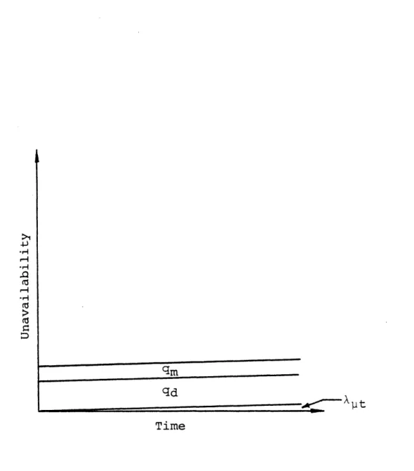
Figure 2.1 is a graphical representation of the
asymptotic unavailability of all types of components other than periodically tested. There are three contributors to the component' s unavailability:
1) Standby failures which occur at a constant rate of X per hour and are detected and repaired with an average downtime of TR. (More commonly known as monitored failures.) These
failure occur to components which perform some type of func-tion during standby, so that failures can be identified when they happen. For illustrative purposes,' the steady state
For a more complete treatment of the probabilistic parameters of components with binary states see, for
>1 .-0 .f-4 qrn qd Time
Figure 2.1. Time Dependent Unavailability of Components Other Than Those Which Must Be Periodically Tested to Re-veal Standby Failures.
unavailability due to the downtime, TR, during which the failures are detected and repaired can be heuristically
derived by recogonizing that, in some increment of time, dt, the unavailability of a component is increased by the proba-bility that it fails in dt and decreased by the probability
that it is repaired in dt. At steady state qm(t) is a
con-stant, qm' and d[q m(t) ] = 0. Therefore:
[1-qm]Xdt - qm(1/TR)dt = 0 (2.2)
Where:
X - Conditional failure rate (assumed constant)
1/TR - Rate at which repairs are completed (assumed to behave as an exponential process)
Rearranging,
XTR
S 1+XTR ~ XTR when XTR<O'l (2.3) 1+TR
2) Transition failures, modeled by a constant time inde-pendent unavailability per demand, qd. These failures occur because of a change in the component's operating conditons
at the time of the accident, including the possibility of operator error.
3) Failures which occur at a rate of per hour during the standby period, but for some reason are not detected until
the component fails to operate under the conditions of the
true demand. The rate at which the component's
unavailabil-ity due to these failures increases can be expressed as
fol-lows:
d[q(t)} = [1-q(t)]X Pdt (2.4)
Where:
X dt = Conditonal probability that the component fails
between t and t+dt, given that it is working at t. [1-q(t)] Probability that the component is working at
time t.
In its most general form X can be a function of time.
(Chap-ter 3 shows how to model time dependent failure rates with a generalized Weibull hazard rate.) For convenience it is
assumed here that X has a constant value. The equation can be rearranged to:
d[q(t)] = Adt (2.5)
[l-q(t)]
and integrated from time 0 to t, yielding
-ln[l-q (t)] + ln[l-q (o)] = X t (2.6)
Since it is assumed that the component was working at t = 0,
q (0) = 0, giving ln(l) = 0. This leads to:
q (t) = 1 - e p't - X t for X t < 0.1. (2.7)
y 91'
The three failure modes are accounted for together because they all behave as a function of just the standby
time. This is not true with periodically tested components, which will be discussed in the next section.
2.2.2 PERIODICALLY TESTED COMPONENTS
There are three major differences between periodically tested components and other types of components:
1) Although X failures occur randomly in time, they are not detected or repaired randomly in periodically tested
components. Repair can not be started until the failure is detected, and failures can not be detected until the compo-nent is tested. Thus detection and repair occur at definite points in time which are controlled by the periodic testing policy.
2) Because periodic testing generally requires that the component be cycled to its active mode to detect
fail-ures, the act of testing can caused additonal failures which contribute the component's unavailability.
3) Whereas TR' the average downtime before a monitored
component can be restored to an operational condition, was a major contributor to the unavailability of monitored
compo-nents, the repair time of periodically tested components is a relatively minor contributor compared to the time during which the failure can have occured but be undetected because
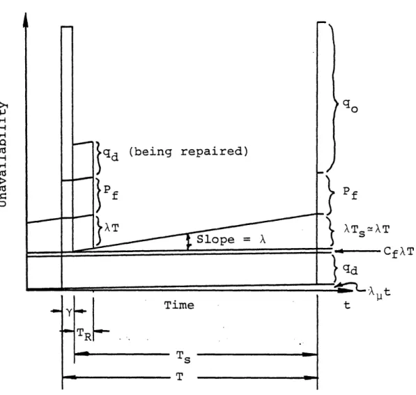
qd (being repaired) .0 Cf f AT ATS~AT qd Y Time t TR[ T T
Figure 2.2. Time Dependent Unavailability of Components Which Must Be Tested to Reveal Standby Failures.
Figure 2.2 shows the time dependence of a periodically tested component. Instead of only one, there are now three distinct time frames for which component unavailability must be determined:
T 3Test period. During this time the component is cycled to its active configuration to verify its operability. If it is found failed during this time it is assumed to remain failed for the entire test period.
T R Repair Period. Failed components are assumed to remain failed until repair is completed, which takes an average of TR time. If components are verified operational by the test, they go back on standby during this time. T s Standby period. For most practical applications, T s
(t+Tr ), so T ~ T, the interval between the begining of consecutive periodic tests. 2
During standby a periodically tested component can be made unavailable for the same reasons as the other types of
components. However, since it is usually idle during
stand-by, failures will not be revealed until the component is
required to perform its function. Assuming that standby failures occur with a constant conditional failure rate of X per hour, the probability that they have occurred increases
in exactly the same manner as that of undetectable failures
modeled by X in Equations (2.4) to (2.7). However, now the
2 In FRANTIC II,
effective time period starts at t , the last time the compo-nent was known to be working. The resulting unavailability
is:
= - -(t-t)
q (t ,t) = 1 - e w ) X(t-t ) (2.8)
X w w
When the component is tested, detectable standby fail-ures are revealed, but other factors also influence the com-ponents unavailability.. The various contributions to a periodically tested component' s unavailability during the test and repair periods are:
q - Demand failures
q (t) - Probability of undetectable standby failures.
This continues to rise throughout the component's life independent of standby, test, and repair (un-less renewal occurs).
qX(t ,tw+T) - Probability that a detectable standby
fail-ure exists at the begining of a periodic test fol-lowing a standby interval of T. (= XT if <0.1) P - Probability that the test causes failures which
require repairs.
q - Probability that a component can not respond to a
true demand while it is being tested.
C - Probability that detectable standby failures are not detected at a periodic test due to human error.
2.3 CURRENT STATUS OF ANALYSIS OF PERIODIC TESTING
2.3.1 REGULATIONS AND STANDARDS
Requirements for periodic testing of standby safety systems are currently set forth in 10 Code of Federal Regu-lations, Part 50, and ANSI/IEEE Std 338-1977, Criteria for the Periodic Testing of Nuclear Power Generating Safety
Systems.
Periodic testing is specifically required in a number of the design criteria set forth in Appendix A to 10 CFR 50.
However, the extent of testing necessary to satisfy the cri-teria is not specified. Instead, general phrases are used. For example, Criterion 18 - "Inspection and testing of elec-tric power systems, " states:
Electric power systems important to safety shall be designed to permit appro-priate periodic inspection of important
areas and features ... to assess the conti- k nuity of the systems and the conditions of
their components.
More specific requirements and criteria for periodic testing are set forth in ANSI/IEEE Std 338-1977. It provides guidance for the development of procedures and documentation,
and the design of equipment necessary for the periodic testing of a nuclear power generating station's protection and power systems. This standard provides an outline of good engineering practice and records requirements to be used in accomplishing
and documenting the tests. The question of test interval is addressed in Appendix Al, which states:
Determination of test intervals based on mathematical relations involving logic,
failure rate data, test duration, and permis-sible system unavailability is covered by IEEE Std 352-1975, Guide for General Princi-ples of Reliability Analysis of Nuclear Power
Generating Station Protection Systems.
Section 7 of ANSI/IEEE Std 352-1975 provides the guidance for the establishment of test intervals. For a single compo-nent system the test interval is expressed as:
0 = 2G/X (2.9)
where:
G Unavailability design goal X Standby failure rate
9 Periodic test interval
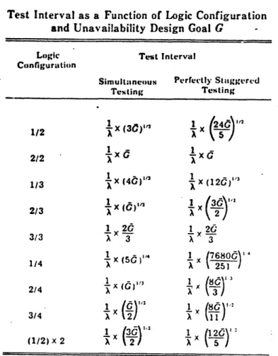
The test intervals for systems of components arranged in common logic configurations are given in Table 4 of the standard,
which is reproduced as Table 2.1.
Equation (2.9) is essentially a rearrangement of the expression for the approximate average unavailability due to detectable standby failures which have occured, but have not yet been revealed by a periodic test. The average unavailabil-ity can be easily found from Figure 2.2. The triangular area represents the increasing probability of unrevealed failures. The average value is half of the maximum, or OX/2 by the current
notation.
The standard does not quantitatively account for downtime unavailability during the test period or the effects of
imperfect testing, although it does mention some of the
Test Interval as a Function of Logic Configuration
and Unavailability Design Goal G
Logic Test Interval
Configuration
Simultaneous Perrectly Staggered
Testing Testing 12X (30)" x 2/2 1/3 x (40) 1jx (12d" 2/3 (12 1 2d 1 20 3/3 3 A 3 x ( )x 6800 1/4 X (A) 251 / 2/4 3 3/4 (1/2) x 2(2
Table 2.1. Table 4 of ANSI/IEEE Standard 352-1975 Test Interval as a Function of Logic Configuration
and Unavailability Design Goal G
lems and tradeoffs the analyst should address. Therefore it should not be applied without supplemental quantitative analy-sis.
2.3.2 PUBLISHED RESEARCH
Many of the tradeoffs to be considered when establishing a periodic test and maintenance policy for a standby safety
sys-tem have been addressed in the literature. However, only spe-cific parts of the problem have been addressed in any one paper and appliciation has been restricted primarily to simple one component systems whose failure rate can be represented by a single distribution, or combinations of components in standard logic configurations, such as 2-out-of-3: Good. 3
Simple Systems With Test Downtime
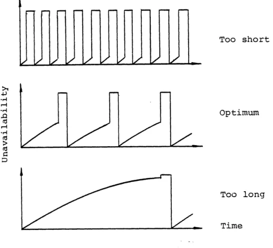
Jacobs [Ja68] and Epstein and Shiff [Ep68] were the first to consider the periodic testing of components which are made unavailable to accomplish their safety function while being tested. They suggested that an optimum test interval could be derived for this type of system. Figure 2.3 illustrates this concept. It shows the unavailability of a single component
system for three different periodic test intervals. At the end of each test the system is known to be working, so the unavail-ability is zero. The failure rate of the component is assumed
constant during standby, and the unavailability rises
exponen-3 The term 2-out-of-3:Good means the system works if 2 of its
3 components are working.
(9~
Too short
Optimum
Too long
Time
Figure 2.3. Example of the Effect of Test Interval on Unavailability.
5 103
Figure 2.4. Unavailability of a Component Subject to Standby Failures and Test Downtime. [Ja68]
>1 H Cd H Cd 10-5 2-10-3 10' 2 5 , j02 2 r, TEST INTERVAL (hr)
tially until the next test is accomplished. Since the safety function of the component is assumed to be bypassed to accom-plish this test, its unavailability rises to one. If the test
interval is very short, the component would be bypassed most of time for testing and would have high unavailability.
Converse-ly, if the component is tested with an extrememly long
interval, its unavailability approaches one and remains there for a very long time. This suggests that there might be a test interval for a given system failure rate and test down time that minimizes the unavailability.
Using this concept, both authors derive an equation which expresses the average unavailability of of a one component sys-tem as:
1-x(1t
Q(S) = 1 [l-e ] (2.10)
Where,
X Conditional failure rate of the system (per hour) , Periodic test interval (hours). [Equivalent to T2
(which has units of days) in FRANTIC]
t Total time that the system is down per cycle due to testing (hours). [Equivalent to (q t ) in FRANTIC] A plot of this equation taken from Jacobs' paper is shown in
Figure 2.4. (Note: Jacobs originally wrote an equation for availability, which he called P(S), but he plotted curves for unavailability, which show the results better. The
ability equation is written here for consistency with the
remainder of the thesis. ) The curves in Figure 2.4 are plotted for a test downtime of 1 hour and two different failure rates. The curves dip through a minimum, indicating that there is an
optimum test interval for a system to be taken out of service for testing. As the failure rate increases, the optimum test interval decreases.
By differentiating equation (2.10), both authors obtain a
simple experession for the optimum test interval in cases which 1/X<<t and X'<0.1:
2t
t= X (2.11)
Note that this equation can be rearranged so that
t(l) = XT (2.lla)
At the optimum test interval the area under the triangle in Figure 2.3 (representing the contribution of standby failures which have occurred but have not been detected) equals the area of the rectangle (downtime contribution of the test which
detects them).
A recent Nuclear Regulatory Commission document, NUREG/CR-2158, duplicates and expands upon the early work
assumptions in deriving the optimal test intervals: (These same assumptions were implicit in earlier papers. )
1. The component has a constant standby fail-ure rate of X per hour.
2. Testing is done periodically and is done on line, i.e., during the test the component could be called upon to operate.
3. During the time of the test, the component is unavailable and unable to respond if called upon to operate.
4. The testing requires an average time peri-od t to complete.
5. Other than the test time r during which the component is unavailable there are no
test-caused failures or degradations such
as those due to human errors.
The equations derived in NUREG/CR-2158 are the same as those derived by Jacobs, with the exception that the approxi-mations for XT and T used to derive Equation (2.11) are also
applied to the unavailability equation and a slightly differ-ent notation is used. The resulting equations are:
q c 0 = IXT + 2 T (2.12)
and
T = 2 (2.13)
0 X
where:
T 0 Optimum test interval