The allocation of attention : theory and evidence

in

2011

with

funding

from

Boston

Library

Consortium

Member

Libraries

HB31

.M415

Massachusetts

Institute

of

Technology

Department

of

Economics

Working

Paper

Series

THE

ALLOCATION

OF

ATTENTION:

THEORY

AND

EVIDENCE

Xavier

Gabaix

David

Laibson

Guillermo

Moloche

Working

Paper

03-31

August

29,

2003

Room

E52-251

50

Memorial

Drive

Cambridge,

MA

02142

This

paper

can

be downloaded

without

charge from

the

Social

Science

Research Network Paper

Collection at

THE ALLOCATION

OF

ATTENTION:

THEORY

AND

EVIDENCE

Xavier Gabaix*

MIT

and

NBER

David Laibson

Harvard

University

and

NBER

Stephen

Weinberg

Harvard

University

Current Draft:

August

29, 2003

GUILLERMO

MOLOCHE

NBER

Abstract.

A

host of recent studies show that attention allocation has important

economicconsequences. Thispaperreportsthefirstempiricaltest ofacost-benefitmodelofthe

endogenousallocationofattention.

The

modelassumesthateconomicagentshavefinitemental

processing speeds and cannot analyze all of the elements in complex problems.

The

model makes tractable predictions about attention allocation, despite the high level of complexity

inour environment.

The

model successfully predictsthe keyempirical regularitiesofattention

allocationmeasuredinachoiceexperiment. In theexperiment, decisiontimeisa scarce resource and attention allocation is continuously measuredusing Mouselab. Subject choices correspond

well tothe quantitative predictionsofthemodel,whicharederivedfrom cost-benefitand option-valueprinciples.

JEL

classification: C7, C9, D8.

Keywords: attention, satisficing, Mouselab.

*Email addresses: xgabaix@mit.edu, dlaibson@arrow.fas.harvard.edu, gmoloche@mit.edu,

swein-ber@kuznets.fas.harvard.edu.

We

thank Colin Camerer, David Cooper, Miguel Costa-Gomes, Vince Craw-ford,AndreiShleifer,Marty Weitzman, threeanonymousreferees, and seminarparticipants atCaltech,

Har-vard,MIT, Stanford, University of California Berkeley,

UCLA,

University ofMontreal,andthe Econometric

Society.

Numerous

research assistants helped run the experiment.

We

owea particular debt to Rebecca Thornton and NataliaTsvetkova.

We

acknowledge financial support from the

NSF

(Gabaix and Laibson

THE ALLOCATION

OF ATTENTION:

THEORY

AND

EVIDENCE

2

l.

Introduction

1.1.

Attention

as

a

scarce

economic

resource. Standard economic models conveniently

assume

that cognition is instantaneous

and

costless.

The

current paperdevelops

and

tests

models

that are based

on

the fact that cognition takes time. Like players in a chess

tournament

or

students taking atest, realdecision-makers need timetosolveproblems

and

oftenencounter

trade-offs because they

work

under time pressure.

Time

almost always has a positive

shadow

value, whether or not formal time limits exist.

Because timeis scarce, decision-makers ignore

some

elements in decisionproblems while

selec-tively thinking about others.1

Such

selective thinking exemplifies the voluntary (i.e. conscious)

and

involuntary processes that lead to attention allocation.2

Economics

is often defined as the study of the allocation of scarce resources.

The

process

of attention allocation, with its consequences for decision-making, seems like a natural topic for

economicresearch. Indeed, inrecent years

many

authors havearguedthatthe scarcityofattention haslarge effects

on economic

choices. Forexample,

Lynch

(1996),

Gabaix

and

Laibson (2001),

and

Rogers (2001) study the effects of limited attention

on consumption

dynamics and

the equity

premium

puzzle.

Mankiw

and

Reis (2002),

Gumbau

(2003), Sims (2003),

and

Woodford

(2002)

study the effects

on

monetary

transmission mechanisms. D'Avolio

and

Nierenberg (2002), Delia

Vigna and

Pollet (2003),

Peng and Xiong

(2003),

and

Pollet (2003) study the effects

on

asset pricing. Finally, Daniel, Hirshleifer,

and

Teoh

(2002)

and

Hirshleifer, Lim,

and

Teoh

(2003) study

the effects

on

corporate finance, especially corporate disclosure.

Some

of these papers analyze

limited attention

from

a theoretical perspective. Others analyze limited attention indirectly,

by

studying its associated

market

consequences.

None

ofthese papers measures attention directly.

The

currentpaperispart ofa

new

literature inexperimentaleconomics that empirically studies

1

Simon (1955)first analyzeddecision algorithms

—

e.g. satisficing

—

that are basedonthe idea that calculation

is time-consuming or costly. See Kahneman and Tversky (1974) and Gigerenzer et al. (1999) for heuristics that simplify problem-solving. See Conlisk (1996)for aframeworkinwhich tounderstandmodelsofthinkingcosts.

Attention"allocation" can bedividedintofour categories: involuntaryperception(e.g.,hearingyournamespoken

across a noisy room at a cocktail party, see Moray 1959and

Wood

andCowan 1995); involuntary central cognitive operations (e.g. trying tonotthinkabout whitebears, but doingso anyway,seeWegner 1989); voluntary perception

(e.g. searchingfora cerealbrandona displayshelf, seeYantis1998); andvoluntary central cognitive operations(e.g.

planning andcontrol of action, seeKahneman 1973, and Pashler andJohnston 1998). See Pashler (1998) for an

excellentoverviewofresearch on attention. The modelthat we analyze in this paper can beapplied toall ofthese

categories of attentionallocation, but wediscuss an application that focuseson conscious attention allocation (the

the decision-makingprocess

by

directlymeasuring attentionallocation

(Camerer

et al. 1993,

Costa-Gomes,

Crawford,

and

Broseta 2001,

Johnson

et al 2002,

and Costa-Gomes and Crawford

2003).

In the current paper,

we

report the first direct empirical test ofan economic cost-benefit

model

of

endogenous attention allocation.

This economic approach contrasts with

more

descriptive models of attention allocation in the

psychology literature (e.g. Payne,

Bettman, and Johnson

1993).

The

economic approach provides

a general

framework

for deriving quantitative attention allocation predictions without introducing

extraneous parameters.

1.2.

Directed

cognition:

An

economic approach

to

attention

allocation.

To

implement

theeconomicapproachinacomputationallytractableway,

we

applyacost-benefit

model

developed

by

Gabaix

and

Laibson (2002), which theycall the directed cognition model. Inthis model,

time-pressured agents allocate their thinking time according to simple option-value calculations.

The

agents in this

model

analyze information that is likely to

be

useful

and

ignore information that is

likely to

be

redundant. For example, it isnot optimalto continue toanalyze a

good

that is almost

surely

dominated by

an alternative good. It is also not optimal to continue to investigate a

good

aboutwhich

you

already have nearly perfectinformation.

The

directed cognition

model

calculates

the economic option-value of marginal thinking

and

directs cognition to the mental activity with

the highest expected

shadow

value.

The

directed cognition

model comes

withtheadvantage of tractability.

The

directedcognition

model

can

be

computationally solved even in highly

complex

settings.

To

gain this tractability, however, the directed cognition

model

introduces

some

partial

myopia

into the option-theoretic

calculations,

and

can thus only approximate the

shadow

valueofmarginal thinking.

Inthis paper

we

show

thatthis approximation

comes

at relativelylittlecost, sincethepartially

myopic

calculations in the directed cognition

model

generate attention allocation choices that

ap-proximate the payoffs from a perfectly rational

—

i.e. infinitely forward-looking

—

calculation of

option values. Because infinite-horizonoption value calculations are not generallycomputationally

tractable

and

because directed cognition is close to those calculations

anyway

(cf.

Appendix

C),

THE ALLOCATION

OF ATTENTION:

THEORY

AND

EVIDENCE

4

1.3.

Perfect

rationality:

an

intractable

model

in

generic

high-dimensional

problems.

Perfect rationality represents a formal (theoretical) solution to

any

well-posed problem.

But

per-fectly rationalsolutions cannot

be

calculated in

complex

environments

and

have limited value as modeling

benchmarks

insuch environments. Researchersinartificialintelligencehave acknowledged

thislimitation

and

taken the extremestep of

abandoning

perfectrationality as

an

organizing

princi-ple.

Among

artificialintelligenceresearchers, the meritofan algorithm isbased

on

itstractability,

predictive accuracy,

and

generality

—

not

by

proximity to the predictions ofperfect rationality.

In contrast to artificial intelligence researchers, economists use perfect rationality as their

pri-mary

modeling approach. Perfect rationality continues to

be

the

most

useful

and

disciplined

modeling

framework

for economicanalysis.

But

alternatives toperfectrationalityshould

be

active

topics ofeconomic study either

when

perfectrationalityis a

bad

predictive

model

or

when

perfect

rationality is not computationally tractable.

The

latter case applies to our attention allocation

analysis.

The

complex

environment that

we

study in this paper only partially reflectsthe even greater

complexityof

most

attention allocationproblems.

But

eveninourrelativelysimplesettingperfectly

rational option value calculations are not computationally tractable.3

Hence

we

focus our analysis

on

a solvable cost-benefit

model

—

directed cognition

—

which

can easily be applied to a wide

range of realistic attention allocation problems. For our application, the merit of the directed

cognition

model

is its tractability, not

any

predictive deviations

from

the perfectly rational

model

ofattention allocation.

We

do not study such deviations

due

to the computational intractability

of the perfectly rationalmodel.

1.4.

An

empirical

analysis of

the directed cognition

model.

This paper

compares

the

qualitative

and

quantitative predictions ofthe directed cognition

model

totheresults of an

exper-iment in

which

subjects solve a generalized choice

problem

that represents avery

common

set of economic decisions: choose one

good from

aset of

N

goods.

Many

economic decisions are special

cases of this general problem.

3

Ofcourse, even whenperfect rationality cannotbesolved, its solutionmightstill bepartiallycharacterizedand

tested.

We

donot takethisapproachin the currentpaper becausethe predictions of the infinite-horizonmodelthat

wehave beenabletoformally derivehavebeenquiteweak(e.g.,ceterisparibus, analyzeinformationwiththe highest variance).

In our experiment, decision time is a scarce resource

and

attention allocation is

measured

continuously.

We

make

time scarce in

two

different ways. In one part ofthe experiment

we

give

subjects

an

exogenous

amount

oftime tochoose one

good from

a set ofgoods

—

achoice

problem

with an exogenous time budget.

Here

we

measure

how

subjects allocatetime as they think about

each good's attributes before

making

a finalselection of

which good

to consume.

In a second part of the experiment

we

give the subjects

an

open-ended sequence of choice

problems likethe one above. Inthis treatment, the subjects keep facing different choiceproblems until atotalbudget oftime runsout.

The amount

oftimea subject choosesforeachchoice

problem

is

now

an endogenous variable. Because payoffs are cumulative

and

each choice

problem

has a

positive expected value, subjects have an incentive to

move

through the choice problems quickly.

But moving

too quickly reduces the quality of their decisions.

As

a result, the subjects trade

off quality

and

quantity.

Spending

more

time

on any

given choice

problem

raises the quality of

the final selection in that

problem

but reduces the time available to participate in future choice

problems with accumulatingpayoffs.

Throughout

the experiment

we

measure

the process of attention allocation.

We

measure

attention allocation within each choice

problem

(i.e.

how

is time allocated in thinking about

the different goods within a single choice

problem

before a final selection is

made

in that choice

problem?). Inaddition, intheopen-ended sequencedesign,

we

measure

attentionallocationacross

choice problems (i.e.

how much

time does the subject spend on onechoice

problem

before

making

a final selection inthat

problem

and

moving

on to the next choice problem?).

Following the lead of other economists

(Camerer

et at. 1993

and

Costa-Gomes, Crawford,

and

Broseta 2001),

we

use the "Mouselab"

programming

language to

measure

subjects' attention

allocation.4

Mouselab

tracks subjects' information search during our experiment. Information

is hidden "behind" boxes

on

a

computer

screen. Subjects use the

computer

mouse

to

open

the

boxes.

Mouselab

records the order

and

duration ofinformation acquisition. Since

we

allow only

onescreen

box

to be

open

at any point in time,the

Mouselab

software enables us to pinpoint

what

informationthe subject is contemplating

on

asecond-by-secondbasis throughoutthe experiment.5

4

Payne,Bettman, and Johnson (1993)developedtheMouselablanguagein the1970's. Mouselabisoneofmany "process tracing" methods. For example, Payne, Braunstein, and Carrol (1978) elicit mental processesby asking subjects to "think aloud." Russo (1978) records eyemovements.

THE ALLOCATION

OF ATTENTION:

THEORY

AND

EVIDENCE

6

Inour experiment,subjectbehavior correspondswelltothe predictions of the directed cognition

model. Subjects allocate thinking time

when

the marginal value ofsuch thinking is high, either because competing goods are close in value or because there is a "large"

amount

of remaining informationtobe revealed.

We

demonstratethis in

numerous

ways. First,

we

evaluatethe pattern ofinformationacquisition withinchoice problems. Second, in the

endogenous

time treatment,

we

evaluate the relationship

between

economic incentives

and

subjects' stopping decisions: i.e.

when

do

subjects stop working

on

one choice

problem

so they

can

move

on

tothe next choice

problem?

We

find that the economic

model

of attention allocation outperforms mechanistic information

acquisition models.

The

marginalvalueofinformation turns out tobethe

most

importantpredictor

of attention allocation.

However, the experiment alsoreveals onerobust deviation

from

the predictions ofthe directed

cognitioncost-benefitmodel. Subject choicesare partially predicted

by

a "boxes heuristic."

Specif-ically,subjects

become more

and more

likelyto

end

analysis ofa

problem

the

more

boxes theyopen,

holdingfixed the economic benefits ofadditional analysis. In this sense, subjects display

a

partial

insensitivity to the particular

economic

incentives in each

problem

that they face.

We

also testmodelsofheuristicdecision-making, but

we

findlittleevidencefor

commonly

stud-ied heuristics, including satisficing

and

elimination

by

aspects. Instead, our subjects generally

allocate their attention consistentlywith cost-benefit considerations, matching the precise

quanti-tative attention-allocation patterns generated by the directed cognition model. Hence, this paper demonstrates that

an economic

cost-benefit

model

predicts

both

the qualitative

and

quantitative

patterns ofattentionallocation.

Section 2 describes our experimental set-up. Section 3

summarizes an

implementable

one-parameter attention allocation

model

(Gabaix

and

Laibson 2002). Section 4

summarizes

the

results ofour experiment

and compares

those results to the predictions of our model. Section 5

concludes.

the Mouselab environment only minimally distorts final choices over goods/actions (e.g., Costa-Gomes, Crawford,

and Broseta 2001 and Costa-Gomes and Crawford 2002). Mouselab's interface does generate "upper-left" and

2.

Experimental

Set-up

Our

experimentaldesignfacilitatessecond-by-second

measurement

ofattentionallocationina basic

decision problem, a choice

among

TV goods.

2.1.

An

TV-good

game.

An

TV-good

game

is

an

TV-row

by

M-column

matrix ofboxes (Figure 1).

Each box

contains a

random

payoff (inunits ofcents) generated with

normal

density

and

zero

mean.

After analyzing

an

TV-good game, the subject

makes

a final selection

and

"consumes" a

single

row

fromthat game.

The

subject ispaid the

sum

ofthe boxes in the

consumed

row.

Consuming

a

row

represents

an

abstraction of a very

wide

class of choice problems.

We

call

this

problem

an TV-good game, since the TV rows conceptually represent TV goods.

The

subject

chooses to

consume

one ofthese TV goods.

The

columns

represent

M

different attributes.

Forexample,consider ashopper

who

hasdecidedtogoto

Walmart

toselect

and buy

atelevision.

The

consumer

faces a fixed

number

of television sets at

Walmart

(TV different

TV's from which

to choose).

The

television sets have

M

different attributes

—

e.g. size, price,

remote

control,

warranty, etc.

By

analogy, theTV

TV's

aretherows ofFigure 1

and

the

M

attributes (inautility

metric) appear in the

M

columns

ofeach row.

Inour experiment, the importanceor variability ofthe attributesdeclines as the

columns

move

from left to right. In particular, the variance decrements across

columns

equal one tenth of the

variancein

column

one. For example, ifthe variance usedto generate

column

oneis 1000 (squared

cents), then the variance for

column

2 is 900,

and

so on, ending with a variance for

column

10 of 100. So

columns on

the left represent the attributes with the

most

(utility-metric) variance, like

screen size or price in our

TV

example.

Columns on

the right represent the attributes with the

least (utility-metric) variance, like

minor

clauses in the warranty.6

So

far our

game

sounds simple:

"Consume

the best

good

(i.e., row)."

To

measure

attention,

we

make

the task harder

by

masking

the contents ofboxes in

columns

2 through

M.

Subjects are

shown

only the

box

values in

column

l.7 However, a subject can left-click

on

a

masked box

in

columns

2 through

M

to

unmask

the valueofthat

box

(Figure 2).

In our experiment,allofthe attributeshave beendemeaned.

We

reveal the value ofcolumnone becauseithelps subjectsrememberwhichrowiswhich. In addition, revealing

columnoneinitializesthegameby breakingtheeight-waytiethatwouldexistifsubjectsbeganwiththeexpectation

THE ALLOCATION

OF ATTENTION:

THEORY

AND

EVIDENCE

8

Only

one

box from columns

2 through

M

can

be

unmasked

at a time. This procedure enables

us to record exactly

what

information the subject is analyzing at every point intime.8 Revealing

the contents ofa

box

does not implythat the subject

consumes

that box.

Note

too that if a

row

is

picked for consumption, then all boxes in that

row

are consumed,

whether

or not they

have been

previously

unmasked.

We

introduce time pressure, so that subjects will not be able to

unmask

—

or will not choose

to

unmask

—

all ofthe boxes inthe game.

Mouselab

enables us to record

which

ofthe

N(M

—

₁₎

masked

boxes the subject chooses to

unmask.

Of

course,

we

also record

which

row

the subject

chooses/consumes for his or her finalselection.

We

study asettingthatreflects realistic

—

i.e. high

—

levelsofdecisioncomplexity. This

com-plexity forces subjects to confront attention allocation tradeoffs. Real

consumers

in real markets

frequently face attention allocationdecisions that are

much

more

complex.

Masked

boxes

and

time pressure capture important aspects ofour

Walmart

shopper's

experi-ence.

The Walmart

shopper selectively attends to information about the attributes of the

TV's

among

which

she is picking.

The

shopper

may

also face

some

time pressure, either because she

has a fixed

amount

of time to

buy

a

TV,

or because she has other tasks

which

she can

do

in the

store ifsheselects her

TV

quickly.

We

explore

both

ofthese types ofcases inour experiment.

2.2.

Games

with

exogenous

and

endogenous time

budgets.

In our experiment, subjects play two different types of JV-good games:

games

with exogenous time budgets

and

games

with endogenous timebudgets.

We

willrefer to these as "exogenous"

and

"endogenous" games.

For each exogenous

game

a game-specifictime budgetisgeneratedfromtheuniformdistribution

over theinterval [10seconds, 49seconds].

A

clock

shows

the subject the

amount

oftime remaining

foreach exogenous-time

game

(see clockin Figure2). This is the case ofa

Walmart

shopper with

a fixed

amount

oftime to

buy

a good.

In

endogenous

games, subjects haveafixed budget oftime

—

25 minutes

—

in

which

to playas

many

different A^-good

games

astheychoose. Inthis design, adjacent A^-good

games

areseparated

When

wedesigned theexperiment, weconsideredbutdidnotadoptadesign thatpermanentlykeeps boxesopen

once theyhadbeenselectedbythe subject. Thisalternativeapproachhas theadvantagethatsubjectsfaceareduced memory burden.

On

theother hand, ifboxes stayopen permanently then subjects have theoption to quickly

—

andmechanically

—

openmanyboxesandonlyafterwardsanalyzetheircontent. Hence, leavingboxesopenimplied

by 20 second bufferscreens,

which

count

toward

the totalbudget of25 minutes. Subjects are free

to

spend

as littleor as

much

timeas they

want on

eachgame, sotime spent

on

each

game

becomes

an

endogenous

choice variable. This is the case of a

Walmart

shopper

who

can

move

on

to other

purchases ifsheselects her

TV

quickly.

We

study

both

exogenous time

games and endogenous

time

games

because these

two

classes

ofproblems

commonly

arise in the real world

and

any attention allocation

model

should be able to handle

both

situations robustly.

Both

types of problems enable us to study within-problem

attention allocationdecisions. Inaddition,the

endogenous

time

games

provide a natural

framework

for studying stopping rules, the between-problemattention allocation decision.

2.3.

Experimental

logistics. Subjects receiveprinted instructionsexplaining the structureof

an

iV-good

game

and

the setup forthe exogenous

and

endogenous games. Subjects arethen given

a laptop

on which

theyread instructions that explain the

Mouselab

interface.9 Subjects play three

test games,

which do

not count toward their payoffs.

Then

subjects play 12

games

with separate exogenous time budgets. Finally, subjects play a

set of

endogenous

games

with ajoint 25-minute time budget. For half ofthe subjects

we

reverse

the order of the exogenous

and endogenous

games.

At

the end oftheexperiment, subjects answer

demographic

and

debriefing questions.

Subjects arepaidthecumulative

sum

ofallrowsthatthey consume. Aftereverygame, feedback

reports therunning cumulative value ofthe

consumed

rows.

3.

Directed

cognition

model

The

previous section describes

an

attention allocation problem. In exogenous games, subjects

must

decide

which

boxes to

unmask

before their time runs out. In

endogenous

games, subjects

must

jointlydecide

which

boxes to

unmask

and

when

to

move

on to the next game.

We

want

to determine

whether

economicprinciples guidesubjects' attentionallocation choices.

We

compare

our experimental data to the predictions of an attention allocation

model

proposed

by

Gabaix and

Laibson (2002). This 'directed cognition'

model

approximates the economic value

ofattention allocation using simple option value analysis.

THE ALLOCATION OF

ATTENTION:

THEORY AND

EVIDENCE

10

The

option value calculations capture

two

types ofeffects. First,

when

many

different choices

are being

compared and

a particular choice gains a large edge over the available alternatives, the

option value of continued analysis declines. Second,

when

marginal analysis yields little

new

information (i.e. the standard deviation of marginal information is low), the economic value of

continued analysis declines.

The

directedcognition

model

captures these

two

effectswith

a

formal

search-theoretic

framework

that

makes

sharp quantitative predictions about attention allocation

choices.

3.1.

Summary

of

the

model.

The

model

canbe broken

down

intothreeiterative steps,

which

we

first

summarize

and

then describe indetail.

Step

1: Calculate the expected

economic

benefits

and

costs of different potential cognitive

opera-tions. For example,

what

is the expected economic benefit of

unmasking

three boxes in the

first row?

Step

2:

Execute

the cognitive operation with the highest ratio of expected benefit to cost. For example, ifexploration ofthe'next'

two

boxes in the sixth

row

hasthe highestexpected ratio of benefit to cost, then

unmask

those

two

boxes.

Step

3:

Return

to step one unless time has run out (in exogenous time games) or until the ratio ofexpected benefit to cost falls

below

some

threshold value (endogenous time games).

We

now

describe the details of this search algorithm.

We

first introduce notation

and

then

formally derive an equationto calculate theexpected economic benefits referredto in step one.

3.2.

Notation.

Since our

games

all have eight rows (goods),

we

label the rows A, B,...,H.

We

will use lower case letters

—

a,b,...,h

—

to track a subject's expectations ofthe values ofthe

respective rows.

Recall thatthe subject

knows

thevalues ofall boxesin

column

1

when

the

game

begins. Thus,

atthebeginning ofthegame,the

row

expectationswillequal the value ofthe payoffinthe left-most

cell of each row. For example, if

row

C

has a 23 in its first cell, then at time zero c

=

23. Ifthe

subject

unmasks

the second

and

third cells in

row

C, revealing cell values of 17

and

-11, then c

3.3.

Step

1:. In step 1 the agent calculates the expected

economic

benefits

and

costs of

dif-ferent cognitive operations. For our application, a cognitive operation is a partial or complete unmasking/analysis of boxes in a particular

row

of the matrix.

Such an

operation enables the

decision-maker to improve her forecast of the expected value ofthat row. In our notation,

O

r

_A

represents the operation, "open

V

additional boxes in

row

A." Because tractability concerns lead

us to limit agents' planninghorizons to only asinglecognitive operationat a time,

we

assume

that

individual cognitive operations themselves can include one or

more box

openings. Multiple

box

openings increase the

amount

ofinformation revealed

by

a single cognitive operator, increase the

option value of information revealed

by

that cognitive operator,

and

make

the (partially myopic)

model

more

forward-looking.10

The

operator

_0\

selects the boxes to

be opened

using a maximal-information rule. In other

words, the

O

v

_A

operator

would

select the

T

unopened

boxes (in

row

.A) that have the highest

variances (i.e. with the

most

information). In our game, this corresponds with left to right

box

openings (skipping any boxes that

may

have

been

opened already).

We

assume

that

an

operator that opens

T

boxes hascostT-k,

where k

isthe cost of

unmasking

a

singlebox.

We

takethis cost to include

many

components, includingthetime involvedin opening

a

box

with a mouse, reading the contents ofthe box,

and

updating expectations.

Such

updating

includes

an

addition operation as well as

two

memory

operations: recalling the prior expectation

and

rememorizing the

updated

expectation.

The

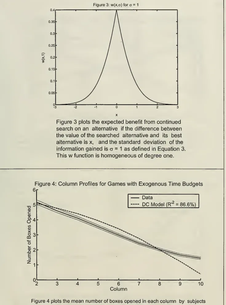
expected benefit (i.e. option value) ofa cognitive operationis given by

:i,)

S <7*g)-|*|*(-M),

w

(x,v)

=

_{*4>{±)-\x\*\-!f\,}

₍₁₎

where

4> represents the standard

normal

density function, <& represents the associated cumulative

distributionfunction,

x

isthe estimatedvalue

gap

between the

row

that isunderconsideration

and

its next best alternative,

and a

is the standard deviation ofthe payoff information that

would

be

10

To gain intuitionfor this effect, consider two goods

A

and B, with E(a)

=

3/2 and E(b)

=

0. Suppose that

openingone boxrevealsoneunitofinformationsothat after thisinformationisrevealedE(a')

=

5/2orE(a')

=

1/2.

Hence,apartiallymyopicagentwon'tseethe benefit ofopening onebox, sincenomatterwhat happens E(a )

>

E(b). However, iftheagentconsidersopeningtwoboxes, thenthereisachancethat E(a') willfall below0, implyingthat gathering theinformationfromtwo boxeswould beusefultothe agent. Analogousargumentsgeneralizeto the case

THE ALLOCATION OF

ATTENTION:

THEORY

AND

EVIDENCE

12

revealed

by

the cognitive operator.

We

motivate equation (1) below, but first present

an example

calculation.

In the

game

shown

in Figure 2, consider a cognitive operator

O

z

_H

that explores three boxes in

row

H. The

initial expected value of

H

is

h

=

—28.

The

best current alternative is

row C, which

has a current payoffof c

=

23.

So

the estimated value

gap between

H

and

the best alternative is

xo

=

\h

—

c\

=

51.

A

box

in

column

n

will revealapayoffr\

_Hn

withvariance(40.8) (1

—

n/10),

and

the

updated

value

of

H

after the threeboxes have

been

opened

will be

h'

=

-28

+

r]

_H2

+

Vm

+

VH4-Hence

the variation revealed

by

the cognitive operatoris

(Q

o _{7 \} To

+

To

+

To)'

i.e.

oo

=

63.2.

So

the benefit of the cognitive operator is

w(xo,&o)

—

7.5,

and

its cost is

To

•

k

=

3k.

We

now

motivate equation (1).

To

fix ideas, consider a

new

game.

Suppose

that the

decision-maker

isanalyzing

row

A

and

will thenimmediately use thatinformationto choose a row.

Assume

that

row

B

would be

the leading

row

if

row

A

wereeliminated, so

row

B

isthe next best alternative

to

row

A.

The

agent is considering learning

more

about

row

A

by executing a cognitive operator

O^.

Executing the cognitive operatorwillenablethe agent to

update

theexpectedpayoffof

row

A

from

a to a'

=

a

+

e,

where

e is the

sum

ofthe values in the

T

newly

unmasked

boxes in

row

A.

Ifthe agent doesn't execute the cognitive operator, her expected payoff willbe

max

(a, b)

THE ALLOCATION

OF ATTENTION:

THEORY AND

EVIDENCE

13

Ifthe agent plans to execute the cognitive operator, her expectedpayoffwill be

E

[max

(a',b)] .

This expectation captures the option value generated

by

being able to pick either

row

A

or

row

B, contingent

on

the information revealed

by

cognitive operator

0^.

The

value of executing the

cognitive operator is the difference

between

the previous

two

expressions:

E

[max

(a',6)]

—

max

(a, b) ₍₂₎

Thisvaluecan

be

representedwitha simple expression. Let

a

representthestandarddeviation

ofthe change in the estimate resulting from applying the cognitive operator:

a

2

=

E{a!

-

a)2.

Appendix

A

shows

that thevalue ofthe cognitive operatoris11

E

[max

(a',_&)]

—

max

(a,b)

— w

(a

—

b,a). ₍₃₎

To

help gain intuition about the

w

function, Figure 3 plots

w

(x,1).

The

general case can be

deduced

fromthe fact that

w

(x,a)

=

aw

(x/a,1)

The

option value

framework

captures

two

fundamental comparative statics. First, the value

of a

row

exploration decreases the larger the gap

between

the active

row and

the next best row:

w

(x,a) is decreasingin \x\. Second, the value of a

row

explorationincreases with thevariability

of the information that will

be

obtained:

w

(x,a) is increasing in a. In other words, the

more

information that is likely to

be

revealed

by

a

row

exploration, the

more

valuable such a path

exploration becomes.

3.4.

Step

2. Step2 executes the cognitive operationwiththe highest ratio ofexpected benefit

to cost. Recall that the expected benefit ofan operator is given

by

the

w(x,a)

function

and

that the implementation cost of

an

operator is proportional to the

number

ofboxes that it unmasks.

THE ALLOCATION OF

ATTENTION:

THEORY AND

EVIDENCE

14

The

subject executes the cognitiveoperator with the greatest benefit/cost ratio12,

w{x

,(To) ...

G

=

m

o

ax

^f^'

(4)

where

k

is the cost of

unmasking

a single box. Since

k

is constant, the subject executes the

cognitiveoperator

O*

=

argmaxiu(xo,o"o)/ro-Appendix

B

contains

an example

ofsuch acalculation.

3.5.

Step

3. Step 3 is a stopping rule. In

games

with

an

exogenous time budget, the subject

keeps returning to step one until time runs out. In

games

with

an endogenous

time budget, the

subject keeps returning until

G

falls below the marginalvalue oftime,

which

must

be calibrated.

3.6.

Calibration

of

the

model.

We

use

two

different

methods

to calibratethemarginal value oftime duringthe endogenous time games.

First,

we

estimate the marginalvalue oftimeasperceived

by

our subjects. Advertisementsfor

the experiment implied that subjects

would

be paid about $20 for theirparticipation,

which would

take about

an

hour. In addition, subjects were told that the experiment

would

be divided into

two

halves,

and

that theywere guaranteed a $5 show-

up

fee.

Using this information,

we

calculate the subjects' anticipated marginal payoff per unit time during

games

with

endogenous

time budgets. This marginal payoff per unit time is the relevant

opportunity cost of time during the

endogenous

time games. Since subjects were promised $5

ofguaranteed payoffs, their expected marginal payofffor their choices during the experiment

was

about $15. Dividing this in halfimplies

an

expectation ofabout $7.50ofmarginal payoffs for the

endogenous

time games. Sincethe

endogenous

time

games

were budgetedtotake25minutes,which

was

known

to thesubjects, the perceived marginalpayoffper secondoftimeinthe experiment

was

(750 cents)/(25 minutes•60 seconds/minute)

=

0.50 cents/second.

12_{Our model}

thus gives a crude but compact way to address the "accuracy vs simplicity" trade-off in cognitive

Since subjects took

on

average 0.98 seconds to

open

eachbox,

we

end

up

with

an

implied marginal

shadow

cost per

box

opening of

(0.50 cents/second)(0.98 seconds /box)

=

0.49 cents/box.

We

also explored a 1-parameter version of the directed cognition model, in

which

the cost of

cognition

—

k

—

was

chosen to

make

the

model

partially fit the data. Calibrating the

model

so it

matches

the average

number

of boxes explored in the endogenous

games

implies

k

=

0.18

cents/box.

Here k

is chosenonlyto

match

theaverage

amount

ofsearchper open-ended game, not

to

match

the order ofsearch or the distribution ofsearch across games.

3.7.

Conceptual

issues. This

model

is easy to analyze

and

is computationally tractable,

im-plying that it can be empirically tested.

The

simplicity of the

model

follows

from

three special

assumptions. First, the

model

assumes that the agent calculates only apartially

myopic

expected

gain

from

executing each cognitive operator. This assumption adopts the approach taken

by

Je-hiel (1995),

who

assumes a constrained planning horizon in a game-theory context. Second, the

directed cognition

model

assumes that the agent uses afixed positive

shadow

value of time. This

shadow

valueoftimeenablesthe agent to tradeoffcurrent opportunities withfuture opportunities.

Third, the directed cognition

model

avoids the infinite regress

problem

(i.e. the costs ofthinking

aboutthinking about thinking, etc.),

by

implicitly assumingthat solving for

O*

is costless to the agent.

Without

some

version of these three simplifying assumptions the

model would

not

be

useful in practice.

Without

some

partial

myopia

(i.e. a limited evaluation horizon for option value

calculations), the

problem

couldnot

be

solvedeither analytically orevencomputationally.

Without

the positive

shadow

value of time, the agent

would

not be able to trade off her current activity

with unspecified future activities

and would

never finish an endogenous time

game

without first

(counterfactually) opening

up

allofthe boxes. Finally, withouteliminating cognitioncosts at

some

primitive stage ofreasoning, maximization models are not well-defined.13

We

return

now

to the first ofthe three points listed in the previous paragraph: the perfectly

See Conlisk (1996) for a description of the infinite regress problem and an explanation of why it plagues all decision cost models.

We

follow Conliskin advocating exogenoustruncationoftheinfinite regressof thinking.

THE ALLOCATION

OF ATTENTION:

THEORY AND

EVIDENCE

16

rational attention allocation

model

is not solvable inour context.

An

exact solution ofthe perfect

rationality

model

requiresthe calculation ofa value function with 17 statevariables: one expected

value for each of the 8 rows, one standard deviation of unexplored information in each of the 8

rows,

and

finally the time remaining in the game. This

dynamic

programming problem

in

R

17

suffers

from

the curse of dimensionality

and would overwhelm

modern

supercomputers.14

By

contrast, the directed cognition

model

is equivalent to 8 completely separable problems, each of

which

has only

two

state variables: x, thedifference

between

the current expectedvalue of the

row

and

the current expected value ofthenext best alternative row;

and

a, the standard deviation of

unexplored information in the row. So the "dimensionality" of the directed cognition

model

is

only 2

(compared

to 17 for the

model

ofperfectrationality).

Although

this paper does not attempt to solve the

model

of perfectly rational attention

allo-cation (or to test it),

we

can

compare

the performance ofthe partially

myopic

directed cognition

model and

the performance ofthe perfectly rational model. Like the directed cognition model,

the perfectly rational

model

assumes that

examining

a

new

box

is costly

and

that calculating the

optimal search strategy is costless (analogous to our assumption that solving for

O*

is costless).

Appendix

C

giveslower

bounds on

the payoffsofthedirectedcognition

model

relativetothepayoffs

ofthe perfectly rationalmodel. Directed cognition does at least

91%

as well asperfect rationality

forexogenous time

games and

at least

71%

aswellasperfectrationalityfor

endogenous

time games.

3.8.

Other

decision

algorithms.

In this subsection,

we

discuss three other models that

we

compare

to the directed cognition model.

The

first

two

models are simple, mechanical search

rules,

which

can be parameterized as variants of thesatisficing

model (Simon

1955).

These

first

two

models are just benchmarks,

which

are presented as objects for comparison, not as serious candidate theories of attention allocation.

The

third

model

—

Elimination

by

Aspects (Tversky

1972)

—

isthe leading psychology

model

ofchoice

from

a set ofmulti-attribute goods.

The Column

model

unmasks

boxes

column by

column, stopping either

when

time runs out (in

14

Approximating algorithms could be developed, but after consulting with experts in operations research, we

concludedthat existing approximation algorithms cannot beused withouta prohibitivecomputational burden. The Gittinsindex (Gittins 1979,Weitzman1979, WeitzmanandRoberts 1980)does notapply here either-formuchthe

samereason itdoes not applyto most dynamicproblems. InGittins'sframework, it iscrucial thatone canonly do onething toarow (an "arm"): accessit. In contrast,in ourgame,asubjectcan domorethanone thingwitha row.

She can explore it further, or takeit andend the game. Henceour game does not fit in Gittins' framework.

We

games

with exogenous time budgets) or stopping according to a satisficing rule (in

games

with

endogenous

time budgets). Specifically the

Column

model

unmasks

all the boxes in

column

2

(toptobottom), thenin

column

3,..., etc. Inexogenous games, this

column-by-column

unmasking

continues until the simulation has explored the

same

number

ofboxes as a 'yoked' subject.15 In

endogenous

games, the

unmasking

continues until a

row

has

been

revealed with

an

estimated

value greater

than

or equal to

A

CoiuTanmodel;

an

aspiration or satisficing level estimated so that

the simulations generate an average

number

ofsimulated

box

openings that

matches

the average

number

of empirical

box

openings (26 boxes per game).

The

Row

model

unmasks

boxes

row by

row, starting with the "best"

row and

moving

to the

"worst" row, stopping either

when

time runs out (in

games

with exogenous time budgets) or

stopping according to a satisficing rule (in

games

with endogenous time budgets). Specifically the

Row

model

ranks the rows according to their values in

column

1.

Then

the

Row

model

unmasks

all the boxes in the best row, thenthe second best row, etc. In exogenous games, this row-by-row

unmasking

continues until the simulation has explored the

same

number

of boxes as

a

yoked

subject (see previous footnote). In endogenous games, the

unmasking

continues until a

row

has

been

revealed with an estimated value greater than or equal to

A

Rowmodel,

an

aspiration

or satisficing level estimated so that the simulations generate

an

average

number

ofsimulated

box

openings that

matches

the average

number

of empirical

box

openings.

A

choice algorithm called Elimination by Aspects

(EBA)

has

been

widely studied in the

psy-chology literature (see

work by Tversky

1972

and

Payne,

Bettman,

and Johnson

1993).

We

apply this algorithm to our decision

framework

to analyze

games

with endogenous time budgets.

We

use the interpretation that each

row

is a

good

with 10different attributes or "aspects" represented

by

the ten different boxes of the row.

Our

EBA

application assumes that the agent proceeds

aspect

by

aspect (i.e.

column by

column)

from

left to right, eliminating goods (i.e. rows) with

an

aspect that falls below

some

threshold value

A

EBA

. This elimination continues, stopping at the

point

where

the next elimination

would

eliminate all remaining rows.

At

this stopping point,

we

pick the remaining

row

with the highest estimated value.

As

above,

we

estimate ^4

EBA

so that

the simulations generate an average

number

of simulated

box

openings that

matches

the average

5

Insuch a yoking, the simulationis tiedto a particular subject. Ifthat subject opens

N

boxesin gameg, then

THE ALLOCATION OF

ATTENTION:

THEORY

AND

EVIDENCE

18

number

of empirical

box

openings.

4.

Results

4.1.

Subject

Pool.

Our

subjectpooliscomprised of388

Harvard

undergraduates. Two-thirds

of the subjects are

male

(66%).

The

subjects are distributedrelatively evenly over concentrations:

11%

math

or statistics;

21%

natural sciences;

20%

humanities;

29%

economics;

and

20%

other

socialsciences. Ina debriefingsurvey

we

asked our subjects toreporttheir statisticalbackground.

Only

15%

report taking

an advanced

statistics class;

40%

report only an introductory level class;

45%

report never having taken astatistics course.

Subjects received a

mean

total payoff of $29.23, with a standard deviation of $5.49. Payoffs

range

from

$13.07 to $46.69.16 All subjects played 12

games

with exogenous times.

On

average

subjects chose to play 28.7

games

under the endogenous time limit, with a standard deviation of

7.9.

The number

of

games

played ranges

from

21 to 65.

Payoffs

do

not systematically vary with experimental experience.

To

get a sense oflearning,

we

calculate the average payoff

X

(k) of

games

played in

round

k

=

1,...,12 oftheexogenous time

games.

We

calculate

X

B

(k) for the exogenous

games

played Before the

endogenous

games and

X

A

(k) for the exogenous

games

played After the

endogenous

games.

We

estimate a separate

regression

X

(k)

=

a

+

fik for the Before

and

After datasets.

We

find that in both regressions,

/3 is not significantly different

from

0,

which

indicates that there is

no

significant learning within

exogenous time games. Learning

would

imply /?

>

0. Also, the constant

a

is statistically

indis-tinguishable across the

two

samples. Playing endogenous time

games

first does not contribute to

any significant learning in exogenous time games.

Hence

we

fail to detect any significant learning

in our data.17

4.2. Statistical

methodology.

Throughout

our analysis

we

report bootstrap standard errors

for our empiricalstatistics.

The

standard errorsare calculated

by

drawing, withreplacement, 500

samples of388 subjects.

Hence

thestandard errors reflect uncertainty arising

from

the particular

16

Payoffsshowlittlesystematicvariation across demographiccategories. Inlight of this, wehave chosentoadopt

the useful approximationthat allsubjects have identical strategies. Relaxing this assumptionis beyond thescope

ofthecurrent paper, butweregard sucha relaxation as an important futureresearch goal.

17

See e.g. Camerer (2003), Camerer and

Ho

(1999) and Erev and Roth (1998) for some examples ofproblems

sample of 388 subjects that attended our experiments.

Our

point estimates are the bootstrap means. In the figures discussed below, the confidence intervals are plotted as dotted lines

around

those point estimates.

We

also calculated

Monte

Carlo

means

and

standard errors for our model predictions.

The

associated standard errors tend to

be

extremely small, since the strategy is determined

by

the

model. Inthe relevant figures (4-9), the confidenceintervals for the

model

predictions arevisually

indistinguishable fromthe means.18

To

calculate measures of fit of our models,

we

generate a bootstrap sample of 388 subjects

and

calculate a fit statistic that

compares

the

model

predictions for that bootstrap

sample

to

the associated data for that bootstrap sample.

We

repeat this exercise 500 times to generate a

bootstrap

mean

fit statistic

and

a bootstrap standard error for the fit statistic.

4.3.

Games

with

exogenous time

budgets.

We

begin

by

analyzing attention allocation

patterns inthe

games

with exogenous time budgets.

Our

analysis focuses

on

the pattern of

box

openings across

columns and

rows.

We

compare

the empirical patterns of

box

openings to the

patterns of

box

openings predicted

by

the directed cognition model.

We

beginwithatrivialprediction ofourtheory: subjectsshould always

open

boxes

from

left to

right, following a declining variance rule. In our experimental data, subjects follow the declining

variance rule

92.6%

of the time (s.e.

0.7%

19). Specifically,

when

subjects

open

a previously

unopened box

in a given row,

92.6%

of the time that

box

has the highest variance ofthe

as-yet-unopened

boxes inthat row. For reasons that

we

explain below, such left-to-right

box

openings

may

arise because of spatial biases instead ofthe information processing reasons implied

by

our theory.

Now

we

consider the pattern ofsearch across

columns

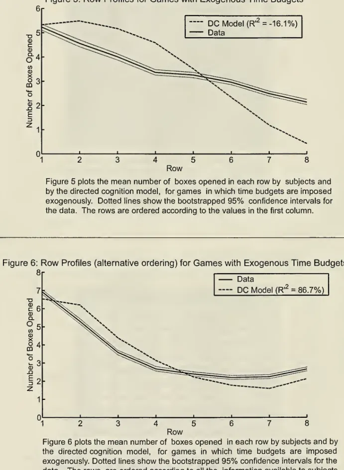
and

rows. Figure 4 reports the average

number

of boxes

opened

in

columns

2-10.

We

report the average

number

of boxes

unmasked,

column by

column, for

both

the subject data

and

the

model

predictions.

The

empirical profile is calculated

by

averaging together subject responses

on

all ofthe

exoge-nous

games

that were played. Specifically, each of our 388 subjects played 12 exogenous games,

1

InFigures4-9, thewidthofthe associated confidence intervals forthe modelsis onaverage only one-halfofone percent of thevalueofthemeans.

19

THE ALLOCATION

OF ATTENTION:

THEORY AND

EVIDENCE

20

yielding a total of388 x 12

=

4656 exogenous

games

played.

To

generate this total, each subject

was

assigned asubset of 12

games from

aset of 160 unique games. Hence, each ofthe 160

games

was

played

an

average of4656/160

~

30 times inthe exogenous time portionofthe experiment.

To

calculatethe empirical

column

profile (andalloftheprofilesthat

we

analyze)

we

count only

thefirst

unmasking

ofeachbox. Soifasubject

unmasks

the

same

box

twice, thiscountsasonlyone

opening.

Approximately

90%

of

box

openings arefirst-time unmaskings.

We

do

not studyrepeat

unmaskings

because they arerelatively rare inour data

and

because

we

are interested in building

a simple

and

parsimonious model. Hence,

we

only implicitly

model

memory

costs as a reduced

form.

Memory

costs are part ofthe (time) cost of opening a

box and encoding/remembering

its

value,

which

includesthecost ofmechanically reopening boxes

whose

values were forgotten.20

Figure 4 also plots the theoretical predictions generated

by

yoked simulations ofour model.21 Specifically, these predictions are calculated

by

simulating the directed cognition

model on

the

exactset of4656

games

played

by

thesubjects.

We

simulate the

model on

each

game

from

this set

of4656

games and

instruct the

computer

to

unmask

the

same number

ofboxesthat

was

unmasked

by

the subject

who

played eachrespective game.

The

analysis

compares

theparticularboxes

opened

by

the subject to the particularboxes

opened

by theyokedsimulation ofthemodel. Figure 4 reports

an

R'2 measure, whichcaptures the extent

to

which

the empirical data

matches

the theoretical predictions. This

measure

is simply the

R

2

statistic22

from

the following constrained regression:23

Boxes(col)

=

constant

+

Boxes{col) +e(col).

Here

Boxes(col) represents the empirical average

number

of boxes

unmasked

in

column

col

and

An

extension ofthisframeworkmightconsider the caseinwhichthememorytechnologyincludememorycapacity constraints ordepreciation ofmemoriesover time.

Seefootnote 15 for a description of ouryokingprocedure. 22

In otherwords,

Y^jcoI \Boxes{col)

-

(Boxes)

—

Boxes(col)

+

(Boxes)]

R

=

_^ :

/ - /_— _\\2

Ylicol [Boxes(col)

—

(Boxes) I

where (} represents empiricalmeans.

3

Inthissection ofthe paper, theconstantis redundant,since thedependent variablehas the same meanas the

independentvariable. However, inthenextsubsectionwewillconsider casesinwhichthisequivalencedoes nothold, necessitating thepresence ofthe constant.

Boxes(col) representsthe simulated average

number

ofboxes

opened

in

column

col.

Note

that col

varies

from

2 to 10, sincetheboxes in

column

1 arealways

unmasked.

This R'2 statisticis

bounded

below

by

—

oo (since the coefficient

on

Boxes(col) is constrained equal to unity)

and

bounded

above

by

1 (aperfect fit). Intuitively, the R'

2

statisticrepresentsthefraction ofsquareddeviations

around the

mean

explained

by

the model. For the

column

predictions, the R'2 statistic is

86.6%

(s.e. 1.7%), implying a very close

match between

the data

and

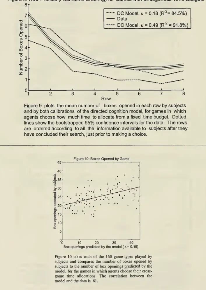
the predictions ofthemodel.

Figure 5 reports analogous calculations

by

row. Figure 5 reports the

number

ofboxes

opened

on average

by

row, withthe rows ranked

by

their value in

column

one. (Recall that

column

one is

nevermasked.)

We

reportthe

number

ofboxes

opened on

average

by

row

for

both

the subjectdata

and

the

model

predictions.

As

above,the

model

predictionsare calculatedusingyokedsimulations.

Figure5 alsoreports

an

R'2

measure

analogoustotheonedescribed above.

The

onlydifference

is that

now

thevariable of interest is

Boxes(row),

the empirical average

number

ofboxes

opened

in

row

row. For our

row

predictions our R'2

measure

is-16.1% (s.e. 9.2%), implying a

poor

match

between

the data

and

the predictions of the model.

The

model

simulations predict too

many

unmaskings

on

the top ranked rows

and

fartoo few

unmaskings on

the

bottom

ranked rows.

The

subjects are

much

less selective

than

the model.

The

R'2 is negative because

we

constrain the

coefficient

on

simulated boxes to

be

unity. This is the only

bad

prediction that the

model

makes. Figure6reportssimilarcalculationsusingan alternative

way

ofordering rows. Figure6 reports

the

number

ofboxes

opened on

average

by

row, withtherows ranked

by

their values atthe end of

each game. For our

row

predictions the R'2 statistic is

86.7%

(s.e. 1.4%).

4.4.

Endogenous

games.

We

repeat the analysis above for the

endogenous

games.

As

dis-cussed in section 3,

we

consider

two

variants ofthe directed cognition

model

when

analyzing the

endogenous games.

We

calibrate onevariant

by

exogenously setting

k

to

match

the subjects' ex-pectedearningsperunittimeintheendogenous games: k

=

0.49 cents/box

opened

(seecalibration

discussionin section3).

With

this calibration, subjects are predicted to

open

15.67 boxes per

game

(s.e. 0.01). In the data, however, subjects

open

26.53 boxes per

game

(s.e. 0.55).

To

match

this

frequency of

box

opening,

we

consider asecond calibrationwith k

=

0.18.

With

this lower levelof

k, the

model

opens the empirically "right"

number

of boxes.

THE ALLOCATION

OF ATTENTION:

THEORY AND

EVIDENCE

22

follow the declining variancerule

91.0%

ofthe time (s.e. 0.8%). Specifically,

when

subjects

open

a previously

unopened box

in a given row,

91.0%

ofthe timethat

box

has the highest variance of

the as-yet-unopened boxes inthat row.

Figure 7 reports the average

number

of boxes

unmasked

in

columns

2-10 in the

endogenous

games.

We

report the average

number

ofboxes

unmasked

by

column

for the subject data

and

for

the

model

predictions with

k

=

0.49

and n

=

0.18.

The

empiricaldataiscalculated

by

averaging together subject responses

on

allofthe

endogenous

games

that were played.

The

theoretical predictions are generated

by yoked

simulations of our model. Specifically,

we

usethedirected cognition

model

to simulate play ofthe 10,931

endogenous

games

that the subjects played.

The

model

generates its

own

stopping rule (so

we

no

longer yoke

the

number

of

box

openings).

Figure7alsoreportstheassociated

R

statisticforthese

column

comparisonsinthe

endogenous

games. For these endogenous games, the

column

R'2 statistic is

96.3%

(s.e. 1.4%) for

n

=

0.49

and 73.1%

(s.e. 4.2%) for

«

=

0.18.

Figure 8 reports analogous calculations

by row

for the

endogenous

games. Figure 8 reports

the

number

ofboxes

opened

on

average

by

row, with the rows ranked

by

their values in

column

one.

We

reportthe

mean

number

ofboxes

opened by row

for boththe subjectdata

and

the

model

predictions. Forthese

endogenous

games, the

row

R'2 statistics are

85.3%

(s.e. 1.3%) for

k

=

0.49

and 64.6%

(s.e. 2.4%) for

k

=

0.18.

Figure 9 reports similar calculations using the alternative

way

of ordering rows. Figure 9

reportsthe

number

ofboxes

opened

on

average

by

row, with the rows ranked

by

theirvalues atthe

end of each game. For these

endogenous

games, the alternative

row

R'2 statistics are

91.8%

(s.e.

0.5%) for

k

=

0.49

and 84.5%

(s.e. 0.8%) for

k

=

0.18.

These

figures

show

that the

model

explains a very large fraction ofthe variation in attention

across rows

and

columns. However, a subset of the results in this section are confounded

by an

effectthat

Costa-Gomes,

Crawford,

and

Broseta (2001) have found intheir analysis. Inparticular,

subjects

who

use the

Mouselab

interface tendto haveabias toward selectingcells inthe

upper

left

cornerofthe screen

and

transitioning

from

left to right as they explorethe screen.

The

up-down component

of this bias does not affect our results, since our rows are

randomly

(figures4

and

7),sinceinformationwithgreatereconomicrelevanceis locatedtoward the left-hand side ofthescreen.

One

way

to evaluate this

column

bias

would

be to flip the presentation of the

problem

dur-ing the experiment so that the rows are labeled

on

the right

and

variance declines

from

right

to left. Alternatively, one could rotate the presentation of the problem,

swapping

columns

and

rows. Unfortunately, theinternal constraints of

Mouselab

make

either of these relabelings

impos-sible.24 Future

work

should usea

more

flexible

programming

languagethat facilitates suchspatial rearrangements. Finally,

we

note that neither the

up-down

nor theleft-right biases influence any

ofouranalyses of either

row

openings (above) or endogenous stopping decisions (below).

4.5.

Stopping

Decisions

in

Endogenous Games.

Almost

all ofthe analysis above reports

within-gamevariationinattentionallocation.

The

analysisabove

shows

that subjectsallocate

most

oftheir attention toeconomically relevant

columns

and

rows within agame,

matching

the patterns

predicted

by

the directed cognitionmodel.

Our

experimentaldesignalsoenables us to evaluate

how

subjects allocate their attention between games. In this subsection

we

focus

on

several measures

ofsuch

between-game

variation.

First,

we

compare

the empirical variation inboxes

opened

per

game

to the predicted variation

in boxes

opened

per game.

Most

importantly,

we

ask whether the

model

can correctly predict

which

games

received the

most

attention

from

our subjects.

Our

experiment utilized 160 unique games,

though

no single subject played all 160 games. Let Boxes(g) represent the average

number

ofboxes

opened

by

subjects

who

played

game

g. Let Boxes(g) represent the average

number

of boxes

opened by

the

model

when

playing

game

g. Inthissubsection

we

analyze thefirst

and

second

moments

ofthe empirical sample

{Boxes(g)}^

1

and

the simulated sample {Boxes(g)}

1

^

1.

Note

that these respective vectorseachhave 160 elements, since

we

areanalyzing game-specific averages.

We

begin

by comparing

first

moments.

The

empirical (equally weighted)

mean

of Boxes(g)

is 26.53 (s.e. 0.55).

By

contrast the 0-parameter version ofour

model

(with

k

=

0.49) generates

a predicted

mean

of 15.67 (s.e. 0.01). Hence, unless

we

pick

k

to

match

the empirical

mean

(i.e.

24

However, one couldleavethelabelsontheleft andhavetheunobserved variances declinefrom righttoleft. In

this design, the displayed cells would have the minimalvariance instead of the maximal variance. Such a design

would eliminate the old left-right bias, but it would create a new bias by making the row "label" appear on the