HAL Id: hal-01093237
https://hal.inria.fr/hal-01093237
Submitted on 10 Dec 2014
HAL is a multi-disciplinary open access
archive for the deposit and dissemination of
sci-entific research documents, whether they are
pub-lished or not. The documents may come from
teaching and research institutions in France or
abroad, or from public or private research centers.
L’archive ouverte pluridisciplinaire HAL, est
destinée au dépôt et à la diffusion de documents
scientifiques de niveau recherche, publiés ou non,
émanant des établissements d’enseignement et de
recherche français ou étrangers, des laboratoires
publics ou privés.
A Fast Ultrasonic Simulation Tool based on Massively
Parallel Implementations
Jason Lambert, Gilles Rougeron, Lionel Lacassagne, Sylvain Chatillon
To cite this version:
Jason Lambert, Gilles Rougeron, Lionel Lacassagne, Sylvain Chatillon. A Fast Ultrasonic Simulation
Tool based on Massively Parallel Implementations. 40th Annual Review of Progress in Quantitative
Nondestructive Evaluation, Center for Nondestructive Evaluation; World Federation of NDE Centers,
Jul 2013, Baltimore, Maryland, United States. �10.1063/1.4865069�. �hal-01093237�
A Fast Ultrasonic Simulation Tool based on Massively
Parallel Implementations
Jason Lambert
∗, Gilles Rougeron
∗, Lionel Lacassagne
†and Sylvain Chatillon
∗∗CEA, LIST, F-91191 Gif-sur-Yvette, France †LRI, Université Paris-Sud, F-91405 Orsay cedex, France
Abstract. This paper presents a CIVA optimized ultrasonic inspection simulation tool, which takes benefit of the power of massively parallel architectures : graphical processing units (GPU) and multi-core general purpose processors (GPP). This tool is based on the classical approach used in CIVA : the interaction model is based on Kirchoff, and the ultrasonic field around the defect is computed by the pencil method. The model has been adapted and parallelized for both architectures. At this stage, the configurations addressed by the tool are : multi and mono-element probes, planar specimens made of simple isotropic materials, planar rectangular defects or side drilled holes of small diameter. Validations on the model accuracy and performances measurements are presented.
Keywords: Ultrasonic Inspection Simulation, Graphical Processing Units, Pencil Method, Kirchhoff Model
INTRODUCTION
Inspection simulation is used in a lot of non-destructive evaluation (NDE) application : from designing new in-spection methods and probes to qualifying methods and demonstrating performances through virtual testing while developing methods. The CIVA software, developed by CEA-LIST and partners is a multi technique platform (Ultra-sonic Testing (UT), Computed Tomography and Radiographic Testing) used to both analyze acquisitions and to run simulations validated against international benchmark [1]. It benefits from semi-analytics models and user friendly GUI to design an inspection case with the help of CAD tools and imaging. However, due to the potential complexity of the configurations, current semi-analytical models based on asymptotic developments takes minutes to hours to run a simulation. Significant efforts are made in the CIVA framework to reduce computation times by working both on models and computational aspects. The works reported here ties in with this general approach.
Nowadays, new massively parallel architectures can empower computational softwares, at the expense of adapting algorithms to the specificities of those architectures to highlight and improve parallel computation steps. The exploita-tion of both multicore-GPP and GPU capabilities results in a new intensively parallel algorithm of simulaexploita-tion of UT inspection [2] [3]. This new model relies on analytical solution to the beam propagation. Its implementations on both architectures use high performances signal processing libraries (Intel MKL on GPP and NVidia cuFFT on GPU). The new model is, however, limited to canonical configurations due to the strict parallelism requirements and to the lack of genericity of analytical beam propagation.
This paper is organized as follows. The first section presents the new model with the specificities of the anylitical solutions and the resulting limitations to the model. Then, GPP and GPU implementations are detailed. In the next section, the validity of this model is tested against real sets of data from the benchmark held at QNDE2013 conference, conducted by the WFNDEC (World Federation of NDE Centers). Furthermore performances are measured with both implementations on high end hardware to provide some sort of fair comparison. Finally, the last section concludes the paper and discusses future works.
UT INSPECTION SIMULATION
This section is divided in three distinct parts toward presenting the model of the fast and massively parallel ultrasonic simulation. An inspection simulation rely on three steps :
• computation of the field transmitted by the probe on the flaw, • diffraction by the defect,
• computation of the field on the sensor for echo synthesis.
Due to Auld’s reciprocity principle, the field diffracted by the defect to te receiving probe can be obtained by coputing the field transmitted by the receiver (used as an emitter) on the defect. This allow to group computations of the field in reception and in emission together. Transmission of the field transmitted by the probe on the flaw, and field/flaw interaction for received echo synthesis.
Field Computation Using Paraxial Ray Tracing Method
The field computation relies on the pencil method, a generic approach for heterogeneous and anisotropic structures. By evaluating the ray path of the beam, from the transducer to the observation point, it is possible to evaluate the time of flight and the amplitude of the contribution of the beam using energy conservation principle on the tube. As seen in Figure 1, the beam may propagate through different materials and cross multiple interfaces : its contributions Ψ is determined by the propagation matrix obtained by multiplying the elementary contributions of each section of the pencil with the initial contribution Ψ0, as shown in equation 1 [4].
Ψ = Lprop1.Lrot1.Linter1.Lprop2.Lrot2.Linter2...Lpropn.Lrotn.Lintern∗ Ψ0 (1)
Solid angle Elementary surface Observation point Axial ray Source point Paraxial ray
FIGURE 1. Ray tube visualization.
In general case, there is no simple solution to determine the ray path from the source to the computation point. However, in isotropic and homogeneous structures, analytical methods can be used to determine ray path. In direct mode, for standard geometrical surfaces, it is possible to determine a polynomial modelizing the path following Snell-Descartes. The roots of this polynomial, whose degree vary from 4th for planar surfaces to 16th for torical surfaces, correspond to the possible solutions for the ray path. They are determined numerically, through Newton’s and Laguerre’s Method [5]. In the case of half-skip mode, ray path can only be determined analytically for planar surfaces and backwalls, through two dimensional Newton’s method solving. Those analytical method allows for a greater regularity benefitings to the requierments of massively parallel architecutes.
Those limits results in an analytical model dedicated only to a specific set of geometries, where the propagation matrix can be fully determined preemptively thus avoiding costly matrix multiplication, for direct and half skip mode. To benefit from highly parallel architecture, this model will rely on a regular pencil distribution over the sampled transducer and a numerical resolution of the analytical equations.
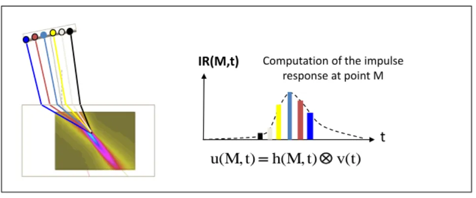
Once the pencils computed on the whole transducer surface, their summation with the application of delay laws results in the computation of the impulse response, as seen in Figure 2. As this model addresses defect response simulation, the field is outlined as the maximum of amplitude, the phase, the corresponding time of flight, the direction of propagation and the wave polarisation.
UT Diffraction Simulation using Kirchhoff Coefficient
UT fields are computed, both in emission and reception (using Auld’s reciprocity theorem), over the studied defect, on a coarse grid.
To sum up the contribution over the defect surface, a finer computation is required (on a finer grid, one order of magnitude finer). The field data (amplitude, phase, time of flight, polarization and direction of propagation) are interpolated from the grid and are used to compute the UT diffraction.
t
IR(M,t) v(t) t) h(M, t) u(M, Computation of the impulse response at point M
FIGURE 2. Summation of the impulse response over the sensor.
This model uses the Kirchhoff model, whose coefficients are valid near specular reflection [6]. All the elementary diffraction contributions computed on the defect contribute to the echo impulse response.
The echo signal is the result of the convolution of the echo impulse response signal an the reference signal.
OVERVIEW OF FAST IMPLEMENTATIONS
In this section, the choices of implementation on both architecture will be discussed under the specificities of the hardware.
GPP Characteristics
Modern day GPP are composed of multiple general purpose cores. Those are aimed at executing independent, heavyweight, tasks. GPP disposes of two parallelism levels.
• A fine grained parallelism relying on specific SIMD instructions (Single Instruction Multiple Data) which execute the same operation on short vectors (128 to 512 bits). For example, with 128-bit vectors, a SIMD instruction can perform simultaneously four additions on four single-precision floating point numbers (32-bit).
• A coarse grained parallelism relying on multithreading to enable multiple logical tasks to reside simultaneously on the GPP. The OpenMP API is aimed at shared-memory parallelism : it creates a thread per GPP core, each with its own stack where locals variables are located but they can also communicate through some shared variable. Its work distribution rely on a succession of sequential sections (with only one active thread) with parallel sections (with all threads active) assembled in a fork-join fashion.
GPP UT simulation implementation
On the GPP, the computations are regrouped by coarse step in order to even the load on each core of the GPP and in order to maximize the reuse of data describing the simulation.
On each step, the OpenMP API is used to parallelize the computations. Moreover the Intel Math Kernel Library (MKL) is used to benefit from fast FFT implementation on the GPP. This library benefits from SIMD instructions available on the processor and rely on a precomputed ”plan” to prepare the coefficients for a specific signal size. Once precomputed, those can be reused as needed for the computations. In order to benefits from the best performances, the signal size has to be determined first and used repeatedly throughout the simulation.
Signal processing is divided in two main steps, each relying on a specific signal size : one concerns the field data computation and the second is responsible for the response signal computation.
Parallel Loop 3x, on x,y,z Parallel Loop Parallel Loop Parallel Loop Parallel Loop START
· Extraction of main direction
· Projection of displacement FFT R2C Convolution FFT C2R FFT R2C FFT C2C Forward Signal Enveloppe FFT C2C Inverse
Enveloppe maximum determination Phase shift computation
END
MKL FFT Methods Memory management Field Inpulse Responses
Sum of elementary contributions to {x,y,z} signals · Memory allocation of those signals · FFT initialisation Size estimation of signal for superposition of elementary
contributions Echo Impulse response
FFT R2C Convolution FFT C2R · Memory allocation of those signals · FFT initialisation Size estimation of signal for
Echo Impulse Response
FIGURE 3. GPP algorithm overview.
NVIDIA GPU Architecture Considerations
NVIDIA released a new programming architecture in 2006 to ease GPGPU on its GPU. This architecture comes with both a programming paradigm and a C-like interface, called Compute Unified Device Architecture (CUDA), to program GPU. A CUDA task is called ”kernel” and it is represented by a C-like function which will be executed once by all threads. With CUDA, GPU are used as coprocessors to their host systems. They dispose of their own memory, off-chip DRAM, called global memory, which is slow to access memory (comparing to GPU frequency), but it is kept alive for the duration of the application allowing communication between kernels without back-and-forth data movement with the host.
A GPU consists of severals Streaming Multiprocessors (SM, 16 on current high end cards). Each one is composed of multiple elements, whose numbers depend on hardware generation, for example :
• CUDA cores for integer and floating-point arithmetic operations; • one or two schedulers to manage threads.
Beside these computing elements, each SM disposes of :
• a rather small (16KB, up to 48KB on recent devices) but fast shared memory on the SM, for exchanges between its cores;
• Special Function Units (SFU) for floating-point transcendentals functions;
• a limited, per SM, set of registers divided between the threads of a kernel at compile-time.
CUDA multiprocessors use the Single Instruction Multiple Thread (SIMT) architecture : each cycle, one instruction is executed by all the cores of a single SM. Threads are grouped into packs of 32 threads, called warps, to be scheduled by each SM. A SM can host multiple warps up to its physical limits, depending of the required configuration form the kernel.
This model is most efficient when each thread in a warp executes the same instruction. In case of divergence, each branch is consecutively executed by the warp, with threads following the other branch doing nothing. Moreover, memory accesses to the different memory of a GPU benefit from data locality by optimizing for contiguous threads of a warp. Each thread disposes of its own program counter and of its own registers. Thread contexts of warps stay on the multiprocessor for the duration of their execution enabling a cheap and fast hardware scheduling of ready warps in spite of execution time and/or latency.
Implementation on the GPU
Due to the high need for computational regularity on GPU, the control flow of this implementation will aim at executing the same task over multiple data and proceed in steps, each corresponding to dedicated kernel. To benefits from highest GPU performances, kernel were developed to use single-precision floating point opretaions (IEEE-754). To perform signal processing operations, this implementation relies on the optimized cuFFT library which is optimized to perform efficiently on large batches of signals. This library establishes a ”plan”, consisting of the precomputed coefficients which are applied to the signals. It is most efficient when performed repeatedly on a batch of signals of the same dimensions (number of signals and signal length), to reuse a previously computed plan.
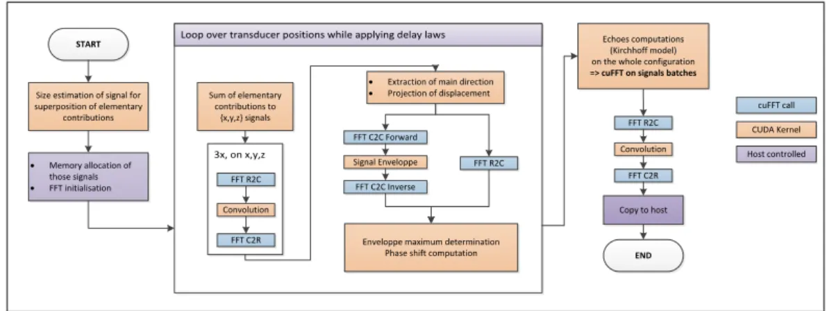
The following Figure 4 illustrate the overall necessary computations steps detailed as follow.
Loop over transducer positions while applying delay laws
3x, on x,y,z START
Size estimation of signal for superposition of elementary contributions · Memory allocation of those signals · FFT initialisation Sum of elementary contributions to {x,y,z} signals
· Extraction of main direction
· Projection of displacement FFT R2C Convolution FFT C2R FFT R2C FFT C2C Forward Signal Enveloppe FFT C2C Inverse
Enveloppe maximum determination Phase shift computation
Echoes computations (Kirchhoff model) on the whole configuration => cuFFT on signals batches
FFT R2C Convolution FFT C2R END Copy to host cuFFT call CUDA Kernel Host controlled
FIGURE 4. GPU algorithm overview.
Signals size determination
The first step of the computation determines the temporal width of temporary data using analytical ray path resolution for time of flight computation. Once the temporal width of the signals is determined, this information is sent back to the host for allocating memory and cuFFT plan creation. This size is the same for all the temporary signals needed for field computation to allow the use of a single cuFFT plan to compute FFT on large batches of signals.
Field data computation
Because of GPU memory limitations, with high end consumer grade hardware disposing of 1.5 GB of memory at most, the whole field computation has to be done on a subset of sensor positions due to the size of temporary data. The following steps are executed on the different subsets of positions by a loop controlled by the host.
For each position, elementary contributions of all the pencils in a specific field point need to be summed following the delay law. The kernel assigns a couple of position/field point to a single CUDA block, to first compute pencils data and store this data in their own shared memory. Threads then loop over the different shots of the delay law to apply delays to the pencils, fetched from shared memory, and proceed with the summation to the signals residing in global memory. It results in completely random accesses to the signal, as there is no way to predict if two distinct pulses will collide in memory due to temporal span : this summation is done using atomic operations. The result of this summation is three impulse responses, one for each displacement coordinate, which are then convoluted with the reference signal.
The main direction is extracted by a new CUDA kernel from those convoluted signals, as a reduction in shared memory performed collaboarively by threads from a single block. This direction is saved for echo computations. The scalar projection of the displacement against this direction is computed.
The envelope of this signal is computed through the use of FFT. Its maximum of amplitude is extracted by another CUDA kernel. Its extraction is again done through a contiguous scan of the signal and a collaborative reduction through
shared memory. It is used to determine the phase shift of the field propagation and to extract the associated time of flight.
Impulse response computation
For each shot and for each sensor position, a response signal is computed. A kernel computes, for a defined mode, the interaction of the received and the emitted field.
The defect is modelized by a set of fine grained sampling point, on witch field information are bilinearly interpolated from previously computed field data. Threads of a block works collaboratively over the whole set of defect points to compute the elementary interaction and sum this data to the global response signal, for a given sensor position and a given shot. As for summing elementary contribution to construct UT field signal data, due to the random nature of this summation to the impulse response, it is necessary to use atomic operations on the signal residing in global memory.
Once computed, the host calls to cuFFT back and forth to convolute the impulse response by the reference signal.
PERFORMANCES OF THE MASSIVELY PARALLEL IMPLEMENTATIONS
To provide a realistic analysis of the results obtained by both implementations, among the limits of this model, realistic set of simulations are studied from the benchmark session of the QNDE 2013 conference.Test cases
The selected cases consist of planar parts of homogeneous isotropic steel, inspected at L45°for several focusing depths :
FBH Serie1 A series of 10 3mm flat bottom holes; FBH Serie2 A series of 6 3mm flat bottom holes;
Notch A back wall breaking notch residing on the planar back wall of the part. The characteristics of those configurations is summed up in Table 1.
TABLE 1. Studied configurations.
Dataset FBH Series 1 FBH Series 2 Notch # of defects 10 FBH 6 FBH 1 notch
Probe 64 channels ↔ 128 samples # of position 361 201 # of delay laws 7 4 UT field sampling # 90 54 100
defect sampling # 4140 2484 12321 Mode L direct L direct Half skip L
Results Validations
To validate the accuracy of the new parallel model, the results of both of its implementations have been studied. As the CIVA 11.0 software is validated against real experiments through benchmarking, especially during the QNDE 2013 conference, its simulations will serve as a point of reference for result validation [7].
The dataset presents an important number of data, for each sensor position and each shot from the delay laws, a response signal is obtained. This analysis focuses on some of the most representative results to highlight the model accuracy on each dataset. Figure 5 illustrate the measurements done on the simulation of the FBH1 series, for the shot corresponding to the echo of maximum of amplitude.
CIVA CPU GPU 0,6dB 0,2dB 0,7dB
FIGURE 5. FBH1 Series - L45°- 25mm depth focusing - FBH @ 35,25,15mm (insonated defects for the law.)
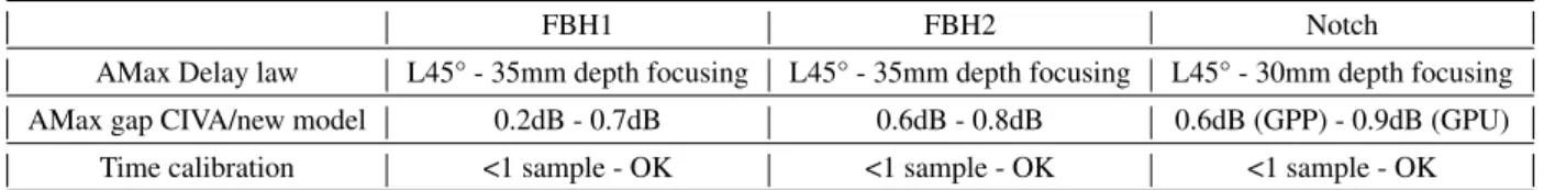
Table 2 presents a summary of the accuracy validation realized on the new model against CIVA 11.0.
TABLE 2. Accuracy analysis summary.
FBH1 FBH2 Notch
AMax Delay law L45° - 35mm depth focusing L45° - 35mm depth focusing L45° - 30mm depth focusing AMax gap CIVA/new model 0.2dB - 0.7dB 0.6dB - 0.8dB 0.6dB (GPP) - 0.9dB (GPU)
Time calibration <1 sample - OK <1 sample - OK <1 sample - OK
Those experiments all fall under 1dB from CIVA results, presenting a gap inferior to the requirements for passing benchmarks against experimental results. Thus, it is possible to validate the new model and its implementations.
Performances
Those two implementations have been benchmarked on high end hardware to aim at a fair evaluation of perfor-mances.
2× GPP Intel Xeon 5590. The machine contains 2 GPP, consisting each of 6 cores 3.47GHz with Hyperthreading (12 logical cores for each GPP) ; it also disposes of 24GB of memory1. This machine is also the one running CIVA
11.0 for reference.
NVidia GeForce GTX580. This high end, consumer grade, GPU disposes of 512 CUDA Cores running @1.544Ghz each, and rely on the Fermi architecture. It disposes of 1.5GB of device memory2. The benchmarked performances do not include GPU initialization nor the transfer of the result from the device back to the host (at most 200ms on the studied cases). Those two elements are dismissed as this implementation is aimed at a fast simulation, memory transfers to the host will be overlapped with computations and the GPU is only initialized once for the whole set.
Experiments. Impulse response simulation is run on the two architectures and on the three sets of data. To provide a reference for current simulation platform performances, the dataset are also run on the CIVA 11.0 software which rely on a general model. However, one has to notice that the CIVA 11.0 generic model is also benefits from multicore architectures through multithreading.
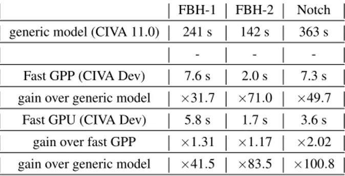
Table 3 shows details of the performances on both implementations. On real data, both implementation of the parallel model perform much faster than CIVA 11.0 generic model. It is noteworthy that most time is spent in signal processing routines : in delay law application to extract field information and in echo impulse response generation.
On the GPP, the signal processing step is costly due to the sheer quantity of memory operations required for computing FFT. Whereas on the GPU, the benefits from the higher parallelism through the cuFFT library are compromised by the cost of the atomic operation required to perform the summation of multiple contributions on a single signal.
1 The compiler used is Intel®C++ Composer XE 2013 Update 5 Integration for Microsoft Visual Studio 2010, Version 13.0.1211.2010 2 The CUDA implementation was compiled and executed with CUDA 5.0 toolkit
TABLE 3. Performances of full parallel implementations against CIVA 11.0 generic model.
FBH-1 FBH-2 Notch generic model (CIVA 11.0) 241 s 142 s 363 s
- -
-Fast GPP (CIVA Dev) 7.6 s 2.0 s 7.3 s gain over generic model ×31.7 ×71.0 ×49.7
Fast GPU (CIVA Dev) 5.8 s 1.7 s 3.6 s gain over fast GPP ×1.31 ×1.17 ×2.02 gain over generic model ×41.5 ×83.5 ×100.8
CONCLUSIONS
This paper describes a new UT inspection simulation tool relying on the computational power of massively parallel architectures. This tool results have been validated on industrial use-cases through the QNDE 2013 benchmark by comparison with the current version of the CIVA software. The new model using an analytical beam propagation computation and computational regularity delivers an accurate simulation of the UT diffraction, under 0.8dB of differences on the benchmark. However, it is restricted to simpler configurations : planar surfaces, isotropic and homogeneous structures. By comparing its performances against CIVA11.0 generic model, the new model obtains an accelerations from ×31 to ×70 on GPP whereas on the GPU, a gain of ×41 to ×101 is shown. The performances shown with those first implementations indicate that interactive simulation is not out of range.
The current implementations are still limited to a subset of canonical configurations. Some extension should be realized to address more configurations, for example : side drilled holes ; other diffraction models which can benefits from the fast field and signal processing computations (GTD, SOV...) ; on the GPU, T mode computations.
Moreover, an analysis aimed at reducing the number of signal processing operations will be performed with the help of CIVA knownledge.
Finally, multiple improvements can be sought to speedup each parallel implementation. For example, the use of SIMD instruction on the GPP to benefit from its fine grained parallel abilities. Besides, by reducing the number of atomic operations in the GPU implementation, performances can improve drastically on signal summation.
Those implementation are the first step toward a fast UT inspection integrated within the CIVA 12 software.
REFERENCES
1. S. Mahaut, S. Chatillon, M. Darmon, N. Leymarie, R. Raillon, and P. Calmon, “An overview of Ultrasonic beam propagation and flaw scattering models in the CIVA software,” AIP, 2010, vol. 1211, pp. 2133–2140.
2. M. Molero, and U. Iturraràn-Viveros, “Accelerating numerical modeling of wave propagation through 2-D anisotropic materials using OpenCL,” 2013, vol. 53, pp. 815 – 822.
3. D. Romero-Laorden, O. Martínez-Graullera, C. J. Martín, M. Pérez, and L. G. Ullate, “Field modelling acceleration on ultrasonic systems using graphic hardware,” 2011, vol. 182, pp. 590–599.
4. N. Gengembre, “Pencil method for ultrasonic beam computation,” in Proc. of the 5th World Congress on Ultrasonics, 2003, pp. 1533–1536.
5. J. Lambert, A. Pedron, G. Gens, F. Bimbard, L. Lacassagne, and E. Iakovleva, “Performance evaluation of total focusing method on GPP and GPU,” in DASIP, IEEE, 2012, pp. 1–8, ISBN 978-1-4673-2089-4.
6. M. Darmon, N. Leymarie, S. Chatillon, and S. Mahaut, “Modelling of scattering of ultrasounds by flaws for NDT,” in Ultrasonic Wave Propagation in Non Homogeneous Media, edited by A. Leger, and M. Deschamps, Springer Berlin Heidelberg, 2009, vol. 128 of Springer Proceedings in Physics, pp. 61–71, ISBN 978-3-540-89104-8.
7. G. Toullelan, R. Raillon, and S. Chatillon, “Results of the 2013 UT Modeling Benchmark Obtained with Models Implemented in CIVA,” in The 40th Annual Review Of Progress In Quantitative Nondestructive Evaluation, 2013.