Impact study of the wastewater treatment plant effluents on fluorescence of coastal zone water using fluorescence EEM-PARAFAC

HAL Id: hal-02555075

https://hal.archives-ouvertes.fr/hal-02555075

Submitted on 27 Apr 2020

HAL is a multi-disciplinary open access archive for the deposit and dissemination of sci-entific research documents, whether they are pub-lished or not. The documents may come from teaching and research institutions in France or abroad, or from public or private research centers.

L’archive ouverte pluridisciplinaire HAL, est destinée au dépôt et à la diffusion de documents scientifiques de niveau recherche, publiés ou non, émanant des établissements d’enseignement et de recherche français ou étrangers, des laboratoires publics ou privés.

effluents on fluorescence of coastal zone water using

fluorescence EEM-PARAFAC

Ibrahim El-Nahhal, Roland Redon, Michel Raynaud, Yasser El-Nahhal,

Stéphane Mounier

To cite this version:

Ibrahim El-Nahhal, Roland Redon, Michel Raynaud, Yasser El-Nahhal, Stéphane Mounier. Impact study of the wastewater treatment plant effluents on fluorescence of coastal zone water using fluo-rescence EEM-PARAFAC. Environmental Science and Pollution Research, Springer Verlag, In press, �10.1007/s11356-020-08842-w�. �hal-02555075�

Impact study of the wastewater treatment plant effluents on fluorescence of coastal zone water using fluorescence EEM-PARAFAC.

EL-Nahhal Ibrahim_​a*​_{, Redon Roland​}a​_{, Raynaud Michel​}a​ _{, EL-Nahhal Yasser​}b ​_{, Mounier Stéphane​}a

a​ _{Université de Toulon, Aix Marseille Univ, CNRS, IRD, MIO - CS 60584, 83041 TOULON}

CEDEX 9 , France

b _{Department of Environmental and Earth Sciences, Faculty of Science, The Islamic}

University-Gaza Palestinian Territory, P.O Box 108

*​_{Corresponding author : ​elnahhal.i@gmail.com​ (I.Y.EL-Nahhal)}

1 3 4 5 6 7 8 9 10 11 12 13 14 15 16 17 18 19 20 21 22 23 24 25 26 27 28 29 30 31 32 33 34 35 36 37 38 39 40 41 42 43 44 45 46 47 48 49 50 51 52 53 54 55 56 57 58

ABSTRACT :

_​

quality. No specific self-differentiating fluorescence signal of the anthropogenic DOM in the

coastal zone is found in the literature. Solar irradiation were conducted on mixed samples of

River water, sea water, wastewater treatment plant effluent. Excitation Emission Matrices of

Fluorescence were used to monitor the fate of wastewater treatment plant effluent. Multilinear

regression of CP/PARAFAC components contribution depending on mixing composition were

done and was excellent. Kinetics of decreasing contribution versus irradiation time were investigated. Second order Kinetics were found for C1 and C2. Distinction between fluorescence signal of endmembers was undoable. Wastewater treatment plant endmember after photodegradation was highly predominant.

Keywords : Fluorescent Organic Matter, EEM-PARAFAC , multilinear regression,

photodegradation, Coastal zone

1. Introduction

Coastal zone is a transitional zone between the terrestrial and oceanic zo _​nes_{​(Huguet et al.}

2009) and mixing zone between marine/oceanic waters inputs and the freshwater riverine inputs

(Parlanti et al. 2000a) _{​. ​Dissolved organic matter (DOM) play an important role in physical,}

chemical functioning of aquatic ecosystems _{​(Hansell 2009) and biogeochemical processes}

(Hansell & Carlson 2014a) and is a heterogenous mixture of organic compounds of both aromatic

and aliphatic nature _{​(Hansell & Carlson 2014b)​. Chromophoric Dissolved Organic Matter}

(CDOM) is a fraction of DOM which can interact with light _{​(Coble 1996a; Coble 2007;​}Lei et al.

2018_{​) and is ubiquitous in aquatic environmental media ​(Nelson & Siegel 2013) with a subgroup}

2 63 64 65 66 67 68 69 70 71 72 73 74 75 76 77 78 79 80 81 82 83 84 85 86 87 88 89 90 91 92 93 94 95 96 97 98 99 100 101 102 103 104 105 106 107 108 109 110 111 112 113 114 115 116 117 118

fluorescing FDOM_{​(Coble 1996b; Mostofa et al. 2012)​. DOM plays a key role in global carbon}

cycle _{​(Hansell 2001) and is highly influenced by continental inputs ​(Fichot & Benner 2012;}

Yamashita et al. 2013) and by autochthonous sources _{​(Romera-Castillo et al. 2011)​. Most of}

organic matter in the coastal zone is of terrestrial origin _{​(Hedges et al. 1997; Parlanti et al.}

2000b)_​.

Human activity has contributed to increased inputs of terrestrial CDOM in aquatic ecosystems

(Massicotte et al. 2017) _{​. Urbanization is increasing and expected to triple between 2000 and 2030}

(Seto et al. 2012) with higher population density and migration to the coastal zone _{​(Hugo 2011a​};

Hugo 2011b)_{​. In turn, it changes land cover, hence quality and quantity of DOM in rivers ​(Seto et}

al. 2012)_{​. Anthropogenic sources of organic matter vary from industrial ​(Carvalho et al. 2008)​,}

agricultural _{​(Manninen et al. 2018)​, wastewater treatment plants effluents ​(Maizel & Remucal}

2017) , landfill leachates _{​(Oloibiri et al. 2017)​. Moreover, it has been found ​(Williams et al.}

2016) that anthropogenic influence on urban watersheds caused distinct DOM composition.

However, contribution of anthropogenic signal of FDOM in coastal zone is not yet well defined

and evaluated in the literature. Biogeochemistry of natural waters is impacted significantly by

photo-reactivity of CDOM _{​(Andrew et al. 2013; Lønborg et al. 2016) since photochemistry}

affects bioavailability of DOM _{​(Moran & Zepp 1997; Oleinikova et al. 2017)​, microbial activity}

(Piccini et al. 2009)_{​and production of DOM of different character ​(Zhu, Yang, et al. 2017)​.}

Partial information can be extracted from global analytical techniques (DOC, TOC, BOD,

etc…) due to complex composition of DOM. And these techniques are time consuming and

require elaborated sample preparation. Optical properties of CDOM and FDOM provides a

valuable tool in delineating DOM sources _{​(Osburn et al. 2016a) and tracking DOM fluxes of}

3 123 124 125 126 127 128 129 130 131 132 133 134 135 136 137 138 139 140 141 142 143 144 145 146 147 148 149 150 151 152 153 154 155 156 157 158 159 160 161 162 163 164 165 166 167 168 169 170 171 172 173 174 175 176 177 178

terrigenous origin into ocean _{​(Osburn et al. 2016b) enables online or real-time monitoring in}

various media _{​(Helms et al. 2013; Cohen et al. 2014)​. There are so many advantages of}

fluorescence spectroscopy which is useful, less time-consuming, inexpensive, precise qualitative

and quantitative technique _{​(Fellman et al. 2010; Zhu et al. 2014) used among varying scientific}

fields _{​(Gao et al. 2017b)​. Excitation Emission Matrix fluorescence spectroscopy (EEM) has}

furthered scientific research in aquatic systems _{​(Kim & Kim 2015; Dainard et al. 2015; Sgroi et}

al. 2017; Cheng et al. 2018) _{​. It enables characterization of optical properties of FDOM due to its}

high sensitivity, good selectivity and non-destruction of samples _{​(Coble 1996c)​. Coupled with}

Canonical Polyadic / Parallel Factor Analysis (CP/PARAFAC) enables deconvolution of

overlapping independent EEM spectra into distinct components _{​(Stedmon & Bro 2008a)​. In}

addition, the use of this technique EEM/PARAFAC in tracing the DOM fractions which is

cost-effective and rapid in chemistry and aquatic ecology fields is in fact a significant advance in

those fields _{​(Stedmon et al. 2003a)​.}

To the best of our knowledge, there is no previously found pattern or specific

self-distinguishing fluorescence signal of anthropogenic organic matter in the coastal zone. The

present study is focussing on wastewater treatment plants effluent discharge in urban river

systems. Laboratory endmember mixing experiments was conducted of river water , sea water

and wastewater treatment plant, to define contributions after mixing and solar irradiation

experiment. The present study is the first of its kind to develop and propose a multivariate linear

regression for the prediction of FDOM signal and its photodegradation kinetic as a function of

the mixing composition and solar exposure.

4 183 184 185 186 187 188 189 190 191 192 193 194 195 196 197 198 199 200 201 202 203 204 205 206 207 208 209 210 211 212 213 214 215 216 217 218 219 220 221 222 223 224 225 226 227 228 229 230 231 232 233 234 235 236 237 238

2. Material and methods

2.1 Sampling Sites

Gapeau river originates at Signes city (43° 17′ 24″ N, 5° 52′ 59″ E) and run till the sea at city

of Hyères (43°06′42″ N, 6°11′33″ E) in southeastern part of France (figure 1) with a length of

34.4 km _{​(Ollier 1972) and watershed of 544 km​} 2 _{​(Ducros et al. 2018) with a pluvial regime.}

River water (RW) was sampled roughly 500 m before wastewater treatment plant which is

located at ( 43°08'38.6"N 6°05'36.1"E) whereas wastewater treatment plant effluent (WW) was

sampled at its output directly. Wastewater treatment plant of La Crau city has a daily volume of

0.17 m_​3​_{/s. Sea water (SW) was sampled at the coastal area of Hyères city at roughly seven meters}

far from beach ( 43°06'10.4"N 6°10'38.3"E ). Plastic bottle of one liter (cleaned with ethanol

100% and three times rinsed with 18.2 MΩ at 25 °C MilliQ water) was used in sampling.

5 243 244 245 246 247 248 249 250 251 252 253 254 255 256 257 258 259 260 261 262 263 264 265 266 267 268 269 270 271 272 273 274 275 276 277 278 279 280 281 282 283 284 285 286 287 288 289 290 291 292 293 294 295 296 297 298

Fig. 1. Locations of sampling sites in Southeastern France. RW , WW , SW are the points from left to right colored in red.

6 303 304 305 306 307 308 309 310 311 312 313 314 315 316 317 318 319 320 321 322 323 324 325 326 327 328 329 330 331 332 333 334 335 336 337 338 339 340 341 342 343 344 345 346 347 348 349 350 351 352 353 354 355 356 357 358

2.2. Materials of irradiation experiment

2.2.1. Filtration

RW , SW , WW samples were filtered using MilliPore filters (Type GNWP 0.20 µm, 47 mm

diameter) and filtration kit pre-rinsed with acidified water (10% HNO_​3​). Filterates were put in a

new one liter dark glass bottle (pre-rinsed with 10 % HNO _​3 and 3 times with 18.2 MΩ·cm at 25

°C MilliQ-water) and transferred to refrigerator at 4 ℃ in the dark. Filtrates were used for

preparation of 15 mixtures. The measured pH for RW, WW ,SW were 7.4 ± 0.4 .

2.2.2. Preparation of mixtures

Fifteen 50 mL quartz vials were washed with reverse osmosis water then transferred to 10 %

HNO_​3 bath for 24 hours then rinsed three times with 18.2 MΩ·cm at 25 °C Milli Q-water. Then

burnt in oven at 450 ℃ for 24 hours to ensure the elimination of organic/inorganic carbon.

Fifteen mixtures were fabricated. The exact mixing percentages for each mixture are summarized

in table S1 in supplementary information SI. Percentages were taken by weight, assuming a

density of 1.00, 1.00 and 1.025 for WW, RW and SW respectively. A serial number was given to

the vial according to its corresponding mixture (table S1). Each vial was shaken gently by hand

to insure homogeneity of mixtures.

2.2.3. Irradiation experiments 7 363 364 365 366 367 368 369 370 371 372 373 374 375 376 377 378 379 380 381 382 383 384 385 386 387 388 389 390 391 392 393 394 395 396 397 398 399 400 401 402 403 404 405 406 407 408 409 410 411 412 413 414 415 416 417 418

The mixtures were prepared in quartz vials which then were transferred on August 28 _​th ₂₀₁₅

in the evening to the roof of laboratory MIO/Toulon University (43° 08' 11.2" N 6° 01' 16.7" E).

These quartz vials were put at sufficient distances to insure receiving same solar irradiation

conditions. The irradiation started on August 28_​th _{2015 (Day zero) and finished on September}

11_​th​ _{2015 for a total of ten days of irradiation.}

2.2.4. Solar irradiation/insolation measurement

Daily solar insolation data were measured on place in volts using photovoltaic cell (Solar Cell

9V/109 mA) for each day of irradiation. A mean irradiance of 2 343 volts per day was detected.

During this period the irradiation is between 5 to 6 kWh.m _​-2 _{corresponding to 39 mW.cm ​}-2

(_{​www.meteofrance.com​).}

2.3. Excitation Emission Matrix EEM fluorescence spectroscopy

2.3.1. Irradiated water Sampling

Three mL aliquots from each 50 mL exposed quartz vial were sampled and transferred into

10x10 mm quartz cell at different irradiation times. EEMs of solar irradiation experiment sample

were performed using fluorescence spectrophotometer (F4500, Hitachi). Ultrapure Perkin Elmer

deionized water was measured to check spectrofluorimeter stability and measure daily the Raman

peak intensity. Scan speed was set at 2,400 nm.min _​-1​_{. Emission spectra were collected at 5 nm}

8 423 424 425 426 427 428 429 430 431 432 433 434 435 436 437 438 439 440 441 442 443 444 445 446 447 448 449 450 451 452 453 454 455 456 457 458 459 460 461 462 463 464 465 466 467 468 469 470 471 472 473 474 475 476 477 478

intervals between 220 and 420 nm, while excitation spectra were measured between 200 and 400 nm at 5 nm intervals. Slit widths for both excitation and emission wavelengths were set at 5 nm.

2.3.2. EEM Data processing

2.3.2.1. Raman measurement

Water Raman scans of Perkin Elmer blanks were measured for each irradiation day (from Aug.

28_​th _{to Sept. 11​}th _{2015) using the same fluorescence spectrophotometer (F4500, Hitachi). Scans}

used an excitation wavelength of 350 nm whereas the emission intensities were measured from

350 nm to 650 nm with a step of 1 nm. Scan speed was 240 nm.mn _​-1_{with the same slit width of}

5 nm on excitation and emission monochromators.

2.3.2.2. Raman Normalization

Each excitation emission matrix values corresponding to each mixture were normalized to the

integrated Raman signal measured at the corresponding irradiation date. The integrated Raman

signal was calculated by integration the area under the curve from 370 nm to 420 nm _{​(Lawaetz &}

Stedmon 2009)_{​ and used for EEMs normalisation.}

Spectral contribution of each CP/PARAFAC components to total EEM fluorescence was

determined using CP/PARAFAC algorithm_{​(Bro 1997; Stedmon & Markager 2005a)​. Finally, the}

150 Raman-corrected EEMs were modelled using a MATLAB software (MathWorks R2015b)

based on Nway toolbox and DOMFluor toolbox_{​(Stedmon & Bro 2008b)​. Raman and Rayleigh}

scattering were removed according to Zepp method _{​(Zepp et al. 2004)​. No inner filter correction}

was done as samples were in linearity domain. Nonnegativity constraints were applied for

9 483 484 485 486 487 488 489 490 491 492 493 494 495 496 497 498 499 500 501 502 503 504 505 506 507 508 509 510 511 512 513 514 515 516 517 518 519 520 521 522 523 524 525 526 527 528 529 530 531 532 533 534 535 536 537 538

CP/PARAFAC components for excitation and emission loadings. Accepted correct number of CP/PARAFAC components and model validation was taken according to evaluation of

CONCORDIA score and split-half analysis. No outliers were found in the dataset and a three

components model was validated. Once decomposition is done, for each mixture, contributions of

each components were normalised to the maximum value in the whole EEM dataset, which is, in

that work, the initial one before the start of solar irradiation for all experiments, according to the

following equation :

C_iTn ₌ c T ni

max(c ) _iT n ∀n (eq.1)

Where :

T_{​n ​}is the n_​th _{day of irradiation.​c​i}

​

Tn _{is value of contribution of CP/PARAFAC component i and}

C_​i​Tn ​_{the normalised to the maximum contribution of CP/PARAFAC component ​i from 1 to 3}

components.

2.4. Multi-linear regression

Considering _{​f​RW ​}, _​f​SW which are the percentage (w/w) of RW and SW in the quartz vial

mixture respectively, a multi-linear regression was conducted for all _​f​RW​, _​f​SW of a fixed

CP/PARAFAC component i for each irradiation day _​T​n​, considering the following general

multilinear regression formula :

10 543 544 545 546 547 548 549 550 551 552 553 554 555 556 557 558 559 560 561 562 563 564 565 566 567 568 569 570 571 572 573 574 575 576 577 578 579 580 581 582 583 584 585 586 587 588 589 590 591 592 593 594 595 596 597 598

Y_​ = _​a​0​ +_​a​1​.X_​1​+_​a​2​._​X​2​+…+_​a​n​.X_​n (eq. 2)

2.4.1. Multilinear regression of three endmember

RW, SW and WW mixture is constrained by mass total sum of three content fraction that

should be equal to 100 according to the following equation :

f_​SW​+_​f​RW​+_​f​WW​=100 (0<_​f​i​<100) (eq.3)

Where _​f​SW​, _​f​RW​, _​f​WW are content fraction of SW, RW and WW in mass respectively. All percent

fractions obviously positive and less than or equal to 100.

Then

f_​WW​ = 100 -_​f​SW​ -_​f​RW (eq .4)

By substituting in eq. 2 for _​f​WW where n=3, the different terms, the following equation can be

obtained :

C_​i​Tn​ _{= ​a​i,0}

​

+ _{​a​i,1​}._{​f​SW​​}+ _{​a​i,2​}._​f​RW​ + _{​a​i,3​}._​f​WW (eq.5)

Where _​C​i​Tn _{is normalised contribution of CP/PARAFAC component number​i​, and​a​i,1}

​

,_{​a​i,2​},_​a​i,3

the respective partial contribution to this contribution by the three endmember SW, RW and

WW. To simplify, _​C​i​Tn_{​ is replaced by ​C*​i}

​​in the next equations

11 603 604 605 606 607 608 609 610 611 612 613 614 615 616 617 618 619 620 621 622 623 624 625 626 627 628 629 630 631 632 633 634 635 636 637 638 639 640 641 642 643 644 645 646 647 648 649 650 651 652 653 654 655 656 657 658

By substituting for _​f​WW​ by its expression in (eq.4) the following equations can be obtained :

C*_​i​ = _{​a​i,0​} + _{​a​i,1​}._​f​SW​ + _​a​i,2._{​​f​RW​} + _{​a​i,3​}.(100 - _{​f​SW​​}- _​f​RW​) (eq.6)

C*_​i​​= _{​a​i,0​​}+_{​ a​i,​.​}f_​SW​ + _{​a​i,2​}._​fRW​ + _{​a​i,3​}.100 - _{​a​i,3​}._​f​SW​ - _{​a​i,3​}._{​f​RW ​}(eq.7)

By arranging similar terms together and taking the common factor, the following equation can be obtained :

C*_​i​ = (_{​a​i,0​}+ _​ai,3​.100) + (_{​a​i,1​} - _{​a​i,3​})._​f​SW​ + (_{​a​i,2​} - _{​a​i,3​})._​f​RW

(eq.8)

By giving a proper term for the constant and newly modified coefficients to account for f _​WW

term as shown :

A_​WW​

i,0​ = (​a​i,0​+​ a​i,3​.100) ​A​WW​i,1​ ​= (​a​i,1​ - ​a​i,3​) A​WW​i,2​​= (​a​i,2​ - ​a​i,3​)

The final multilinear regression equation is obtained as a function of two content fractions of

two endmembers :

C*_​i​​= _​A​WW_​

i,0_​​+ ​A​WW​i,1_​.​f​SW_​ + ​A​WW​i,2_​.​f​RW ​(eq.9)

12 663 664 665 666 667 668 669 670 671 672 673 674 675 676 677 678 679 680 681 682 683 684 685 686 687 688 689 690 691 692 693 694 695 696 697 698 699 700 701 702 703 704 705 706 707 708 709 710 711 712 713 714 715 716 717 718

Where _​A​WW_​

i,0 , ​A​WW​i,1and ​A​WW​i,2 represent multilinear regression coefficients related to mixing

equation when_​f​WW is expressed in terms of content fraction of the other two endmembers ( _​f​RWand

f_​SW​). Any circular permutation can not yield the _{​a​i,*​​}coefficients independently.

A_​WW_​

i,0 is the constant in the multilinear regression equation which contains information about

WW effect in the multilinear regression, _​AWW​

i,1​is the coefficient of of content fraction of SW

endmember which not only represent its effect but also the effect of the wastewater treatment

plant effluent WW, _​A​WW​

i,2​is the coefficient of of content fraction of RW endmember which not

only represent its effect but also the effect of WW. Determination of_​A​WW_​

i,0,​A​WW​i,1and​A​WW​i,2​was

done for each exposition day.

2.5. Kinetics

The measured irradiation in volts was used as a proxy for photodegradation reaction time . The

determination of the kinetic order of the multilinear regression parameters/coefficients for all _​T​n

was conducted. These multilinear regression are expressed mathematically as a function of volts : A_​WW​ i,0_​ (V) A_​WW​ i,1​ (V) A_​WW_​ i,2​(V) (eq.10)

Where _{​V is received solar irradiation in Volts (V) at each day ​T ​n​}. CP/PARAFAC contribution

during irradiation experiment can be expressed as a function of content fraction of two

endmember depending on V, which enable kinetic study:

13 723 724 725 726 727 728 729 730 731 732 733 734 735 736 737 738 739 740 741 742 743 744 745 746 747 748 749 750 751 752 753 754 755 756 757 758 759 760 761 762 763 764 765 766 767 768 769 770 771 772 773 774 775 776 777 778

C*_​i​ (V)_​ = _​A​WW​

i,0_​ (V) ​+ ​A​WW​i,1_​(V)​ . ​f​SW_​ + ​A​WW​i,2_​(V)​ . ​f​RW (ep.11)

The zeroth, 1st , 2nd and 3rd order kinetics were calculated and compared to find out the most

linear model which fits the data _{​(Wright 2004)​.}

14 783 784 785 786 787 788 789 790 791 792 793 794 795 796 797 798 799 800 801 802 803 804 805 806 807 808 809 810 811 812 813 814 815 816 817 818 819 820 821 822 823 824 825 826 827 828 829 830 831 832 833 834 835 836 837 838

3. Results and Discussion

3.1. EEMs Results

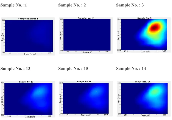
Figure 2. shows the excitation emission matrices EEM of fluorescence for the samples

numbers 1, 2, 3, 13, 14, 15 which are described in table 2. These EEMs are shown after the

removal of Rayleigh and Raman scattering and Raman normalization.

Sample No. :1 Sample No. : 2 Sample No. : 3

Sample No. : 13 Sample No. : 15 Sample No. : 14

Fig. 2. The excitation emission matrices of Samples number 1 , 2 ,3, 13 , 14 and 15 whose

composition is (100,0,0), (0,100,0) ,(0,0,100), (50,0,0), (0,50,0) and (0,0,50) respectively (table S1) 15 843 844 845 846 847 848 849 850 851 852 853 854 855 856 857 858 859 860 861 862 863 864 865 866 867 868 869 870 871 872 873 874 875 876 877 878 879 880 881 882 883 884 885 886 887 888 889 890 891 892 893 894 895 896 897 898

Split-half analysis was conducted for three subsets of the EEM-dataset which asserted the

non-existence ”finding” of any protein-like fluorescent signal. That’s because the CP/PARAFAC

algorithm doesn’t capture what’s already not there.

3.2. CP/PARAFAC decomposition results

CORCONDIA analysis showed drop down between four components and five, from near 70 %

to less than or around 30 % which surpasses acceptable threshold of 60% where as it showed a

value of 80.75 % for three components, indicating that a three-factor model was appropriate. The

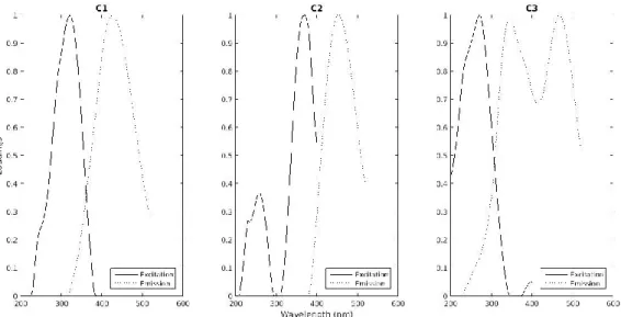
split-half analysis confirm this three components model. Spectral contour plots of components

and their corresponding loadings for both the excitation and the emission wavelengths are shown

in figure 3. C1 C2 C3 16 903 904 905 906 907 908 909 910 911 912 913 914 915 916 917 918 919 920 921 922 923 924 925 926 927 928 929 930 931 932 933 934 935 936 937 938 939 940 941 942 943 944 945 946 947 948 949 950 951 952 953 954 955 956 957 958

Fig. 3. Contour plots of CP/PARAFAC components found in EEM dataset. Spectral loadings

of excitation and emission wavelengths of the three identified CP/PARAFAC in the present

study.

Description of excitation and emission pairs of main peak positions for CP/PARAFAC

components are summarized in Table 1 and compared to previously identified components and

peaks in the literature.

17 963 964 965 966 967 968 969 970 971 972 973 974 975 976 977 978 979 980 981 982 983 984 985 986 987 988 989 990 991 992 993 994 995 996 997 998 999 1000 1001 1002 1003 1004 1005 1006 1007 1008 1009 1010 1011 1012 1013 1014 1015 1016 1017 1018

Table 1

Descriptions of CP/PARAFAC components and comparison with literature

Component λ_EX/λ_EM (nm) Description and references in literature

Component C1 320/425 Component 4 _{​(Stedmon et al. 2003b)​ : terrestrially derived}

organic matter

Peak C _{​(Coble 1996d; Coble et al. 1998)​ : visible humic-like}

Component 2 _{​(Yamashita et al. 2008a)​ : terrestrial}

humic-like

Component 4 _{​(Yamashita et al. 2008b)}

Component C2 370/455 Component 3 _{​(Stedmon et al. 2003c)}

Component G3 _{​(Murphy et al. 2011a)}

Component 3 _{​(Li et al. 2014a)}

Component 7 _{​(Osburn et al. 2016a)}

Component 5 _{​(Baghoth et al. 2011)}

Component 1 _{​(Zhu et al. 2017a)​ Humic-Like}

Component 3 _{​(Yamashita et al. 2008c)​ : Humic-like}

component Component C3 270/(340)

470

Peak T : Tryptophan like fluorescence _{​(Coble 1996d)}

Q2 _{​(Cory & McKnight 2005)}

Small resemblance to C6 _{​(Zhou et al. 2013)​ which was}

Oil-related, degradation product

18 1023 1024 1025 1026 1027 1028 1029 1030 1031 1032 1033 1034 1035 1036 1037 1038 1039 1040 1041 1042 1043 1044 1045 1046 1047 1048 1049 1050 1051 1052 1053 1054 1055 1056 1057 1058 1059 1060 1061 1062 1063 1064 1065 1066 1067 1068 1069 1070 1071 1072 1073 1074 1075 1076 1077 1078

Based on maximum peak position, these three components have been previously identified

(Table 1). C1, showed an excitation maximum at 320 nm and an emission maximum at 425 nm

and a range of excitation emission wavelengths (Ex=300-350 nm, Em=400-450 nm). Previous

studies have associated this component to UVA humic-like fluorescent CP/PARAFAC

component and Peak C _{​(Coble 2007) and peak “∝” ​(Parlanti et al. 2000c; Sierra et al. 2005)​. It}

was previously found from terrestrial, anthropogenic, agricultural sources_{​(Stedmon et al. 2003d;}

Stedmon & Markager 2005b) _{​. C2 component showed an excitation maximum at 370 nm and an}

emission maximum at 455 nm and a range of excitation emission wavelengths (Ex=340-400 nm,

Em= 400-500 nm). In addition, spectra of C2 resembles spectra of component “G3” which has

Ex_​max​=350 nm, Em_​max​=428 nm in _{​(Murphy et al. 2011b) who have attributed it to wastewater or}

nutrient enrichment tracer. This component has also been identified as humic-like component,

similar to “C3” _{​(Li et al. 2014b) which had two excitation maxima (at 250, 350 nm)}

corresponding to the same emission maxima (at 440 nm). Furthermore, C2 has very similar

spectra to “C7” from recycled water studies, which included samples of wastewater, treated

water, gray water _{​(Osburn et al. 2016b)​. C3, showed an excitation maximum at 270 nm and an}

emission maximum at 340 nm and 470 nm which is bimodal in emission. It’s range of excitation

emission wavelengths is Ex=200-300 nm, Em=300-500 nm. The 1 _​st _{peak (270/340 nm) is near}

the tryptophan-like peak_{​(Coble 1996e)​. This component could be protein-like component but it}

resembles noise. 19 1083 1084 1085 1086 1087 1088 1089 1090 1091 1092 1093 1094 1095 1096 1097 1098 1099 1100 1101 1102 1103 1104 1105 1106 1107 1108 1109 1110 1111 1112 1113 1114 1115 1116 1117 1118 1119 1120 1121 1122 1123 1124 1125 1126 1127 1128 1129 1130 1131 1132 1133 1134 1135 1136 1137 1138

3.3. Multivariate Linear Regression Parameters

Numerical values of multilinear regression coefficients (eq. 9) for each CP/PARAFAC

component C1, C2 and C3 are the following for time zero, i.e. Aug. 28_​th​ _2015.

For

C1 = 100.45 - 0.99 *_​f​SW​ -0.93*_{​f​RW ​​} with coefficient of determination r_​2​ _{value of 0.99}

C2 = 98.67 -0.97 *_{​f​SW ​}-0.92*_{​f​RW ​}with r_​2​ _{value of 0.99}

C3 = 72.84 -0.66 *_{​f​SW ​}-0.64*_{​f​RW ​}with r_​2​ _{value of 0.84}

From the above substituted equations, it can be seen that the correlation coefficient is greater

than 0.95 for C1 and C2 indicating multilinear regression is excellent. Values of the intercept are

always greater than values of coefficients of _​f​SWand_​f​RW​by two orders of magnitude. These values

of the parameters/coefficients of the multilinear regression are calculated after the Raman unit

corrections of the EEM-dataset. Knowing that values of the intercept account for effect of _​f​WW on

contribution of CP/PARAFAC component, these results show that contribution of

CP/PARAFAC component decreases with increasing_​f​SW or_​f​RW​. Indeed, all of coefficients _​f​SW​,_​f​RW

have negative sign. As a consequence, it can be observed that for _{​f​SW ​}=100 or _​f​RW​=100,

contributions are weak compared to the f _​WW​=100, i.e _​f​SW​=_​f​RW​=0. These indicated that most of

fluorescence contributions are due to WW endmember considering the blank fluorescence _​a​i,0 as

negligible. Considering that WW is the principal contributor to the all components contribution,

there is no specific end member response for SW and RW in these mixtures.

20 1143 1144 1145 1146 1147 1148 1149 1150 1151 1152 1153 1154 1155 1156 1157 1158 1159 1160 1161 1162 1163 1164 1165 1166 1167 1168 1169 1170 1171 1172 1173 1174 1175 1176 1177 1178 1179 1180 1181 1182 1183 1184 1185 1186 1187 1188 1189 1190 1191 1192 1193 1194 1195 1196 1197 1198

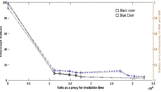
Fig. 4. The variation with irradiation time (volts as proxy for time) of the parameters of

multilinear regression ( Intercept , absolute values of _{​f​RW ​}coefficient, absolute values of _​f​SW

coefficient) for C1 and C2 .

The intercept and the coefficients of _​f​RWand _​f​SW of CP/PARAFAC C1 (shown in black) has a

faster degradation rate than their counterparts of C2 (shown in blue) as shown in figure 4. which

in agreements with the values of the kinetic rate constants as shown in table 6 .

3.4. Determination of kinetic decay coefficient and its kinetic order

The irradiation experiment showed continuous decrease of fluorescence signal with irradiation

time. No stable signal or significant fluorescence increase was observed like in other works _​(;

Song et al. 2015; Zhu et al. 2017b) _{​. Integrated rate law linear equations of zero​} th​_{, 1​}st​_{, 2​}nd​_{, and 3 ​}rd

kinetic order were investigated for each coefficient_​A​WW_​

i,0​, ​A​WW​i,1 and​A​WW​i,3 to determine kinetics

of photodegradation for each multilinear regression parameter. Kinetic order was chosen

according to the best coefficient of determination according to kinetic integrated order law,

21 1203 1204 1205 1206 1207 1208 1209 1210 1211 1212 1213 1214 1215 1216 1217 1218 1219 1220 1221 1222 1223 1224 1225 1226 1227 1228 1229 1230 1231 1232 1233 1234 1235 1236 1237 1238 1239 1240 1241 1242 1243 1244 1245 1246 1247 1248 1249 1250 1251 1252 1253 1254 1255 1256 1257 1258

selecting linear correlation coefficient which must be greater than the threshold 0.75 after

eliminating outliers _{​(Wright 2004)​. Results are presented in table 2 for kinetic order, and kinetic}

constant are presented in table 3. It was found that all kinetics are 2 _​nd_{order and are in agreement}

with a previous work _{​(Yang et al. 2014)​. Long term photodegradation of fluorescent organic}

matter is a bimolecular reaction probably involving exited organic matter and organic matter

itself. Other work assumed first order kinetic under solar simulated irradiation _{​(Wu et al. 2016)}

but experiment were done during 12h and under 2.80 mW.cm_​-2 _{(visible) and 70.00 mW.cm​}-2​_,

corresponding to the starting point of present irradiation experiment that could be assumed as

pseudo-first order kinetic. On the same time, Hee et al 2018 didn’t find variation with a 4,2

mW.cm_​-2​_{, during 10 hours of exposition.}

Table 2

Kinetic order of coefficients of multilinear regression for each CP/PARAFAC with its

corresponding _​r​2 _{​of 2​}nd_{order kinetics to the right. “NA” means that correlation coefficient for 2 ​}nd

order rate was less than 0.75, and was dismissed.

C1 C2 C3 A_​WW​ 1,0 interpt r_​2 _A​WW​ 1,1 (f​SW​) r_​2 _A​WW​ 1,2 (f​RW​) r_​2 _A​WW​ 2,1 interpt r_​2 _A​WW​ 2,1 (f​SW​) r_​2 _A​WW​ 2, 2 (f​RW​) r_​2 _A​WW​ 3,1 interpt A_​WW​ 3,2 (f​SW​) A_​WW​ 3,3 (f​RW​) 2 0.94 2 0.95 2 0.96 2 0.83 2 0.78 2 0.82 NA NA NA

Table 2 clearly shows that the kinetic order of photodegradation reaction for each parameter of

the multi-linear regression for CP/PARAFAC components C1 and C2 are second-order kinetics

and the corresponding coefficient of determination r _​2 _{is greater than 0.75 . For the third}

22 1263 1264 1265 1266 1267 1268 1269 1270 1271 1272 1273 1274 1275 1276 1277 1278 1279 1280 1281 1282 1283 1284 1285 1286 1287 1288 1289 1290 1291 1292 1293 1294 1295 1296 1297 1298 1299 1300 1301 1302 1303 1304 1305 1306 1307 1308 1309 1310 1311 1312 1313 1314 1315 1316 1317 1318

CP/PARAFAC component C3 , no order could be found since this component is noise-like component (table 3) and it was neglected from the analysis.

Table 3

Kinetic constant for coefficients of multilinear regression for each CP/PARAFAC component.

Values in parenthesis are standard deviation for kinetic constant. All values should be

multiplied by 10_​6 ​_{. NA : Not Available}

C1 C2 C3 A_​WW​ *,0 interpt 9.68(1.00) 4.85(0.78) NA A_​WW​ *,1 (f_​SW​) -987.35(92.31) -542.80(101.97) NA A_​WW​ *,2 (f_​RW​) -977.67(83.84) -552.56(91.70) NA

Values of kinetic constant for intercept for both C1 and C2 are smaller than those values

of kinetic constant for _​A​WW_​

1,1 which is coefficient of​ ​f​SW and ​A​WW​1,2 which is coefficient of​ ​f​RW

(table 3). This result could be interpreted as follows: C1 and C2 contributions of RW and SW are

more sensitive to photodegradation than WW which in turn decays approximately 100 times

slower under irradiation suggesting its dominance in the residual fluorescence of both C1 and C2

after long term irradiation. Hence even if there is no specific endmember CP/PARAFAC

23 1323 1324 1325 1326 1327 1328 1329 1330 1331 1332 1333 1334 1335 1336 1337 1338 1339 1340 1341 1342 1343 1344 1345 1346 1347 1348 1349 1350 1351 1352 1353 1354 1355 1356 1357 1358 1359 1360 1361 1362 1363 1364 1365 1366 1367 1368 1369 1370 1371 1372 1373 1374 1375 1376 1377 1378

contribution, it exist a photosensitivity difference between WW and RW or SW. Under long

irradiation, WW contribution is more resilient and refractory to photodegradation. This difference

of behavior depending on endmember mixing was already observed between terrestrial and

autochthonous organic matter _{​(Zhu et al. 2017c)​. Small differences were also observed on}

reclaimed water using fluorescence matrix regional integration between humic-like and

protein-like under high irradiation _{​(Wu et al. 2016)​. Therefore, it can be said that wastewater}

treatment plant fluorophores are somehow similar to natural fluorophores but more refractory to

photodegradation. Anthropogenic dissolved organic matter, in the present study, remains and

constitute the greatest contribution of CP/PARAFAC components along irradiation process.

Fluorescence signal going to the coastal zone should mainly come from WW endmember.

Comparing C1 versus C2 degradation kinetic, it was observed that humic-like FDOM is more

reactive than protein-like FDOM _{​(Yang et al. 2014)​. However, results above demonstrated that}

it’s not so simple. CP/PARAFAC components are constituted by several types of FDOM

fluorophores which behave differently depending on their origin and photosensitivity.

​(Timko et al. 2015) found increasing rates of photochemical fluorescent DOM loss with

increasing pH studied thru measurements on the EEMs not between the parameters of multilinear

regression between CP/PARAFAC components and mixing composition . However, _{​pH of RW ,}

SW and WW were constant (_​pH​=7.4 ± 0.4) in this study suggesting no effect of _{​pH in the results}

of the kinetic analysis

24 1383 1384 1385 1386 1387 1388 1389 1390 1391 1392 1393 1394 1395 1396 1397 1398 1399 1400 1401 1402 1403 1404 1405 1406 1407 1408 1409 1410 1411 1412 1413 1414 1415 1416 1417 1418 1419 1420 1421 1422 1423 1424 1425 1426 1427 1428 1429 1430 1431 1432 1433 1434 1435 1436 1437 1438

4. Conclusions

In this study, fluorescent conservative behaviour and natural solar changes on three endmember mixing laboratory experiment were investigated leading to the following conclusions

(1) Multilinear regression model for contribution of CP/PARAFAC components is excellent and

could be done for the three endmembers in addition to being able to study the kinetic evolution.

(2) Two of the three fluorescence CP/PARAFAC extracted component (C1 “terrestrial humic

like” and C2 “humic-like of longer wavelength”) showed a second order photodegradation

toward the irradiation process whatever the endmember mixture composition.

(3) Search for specific self-distinguishing fluorescence signal or signature for river water,

wastewater treatment plants and sea water couldn’t be done in this work, which could be

attributed to the complexity of the anthropogenic and natural dissolved organic matter.

(4) The fluorescence signal of wastewater treatment plant effluent is predominant in the studied

coastal zone, according to the results of photodegradation kinetic constant which favour anthropogenically-impacted organic matter contribution (100 times less sensitive to

photobleaching). However, its exact contribution couldn’t be found due to inability to calculate

or find its coefficient _{​a​i,3​​} in the multilinear regression model independently.

(5) In human impacted coastal zone, residual fluorescent organic matter comes from wastewater

treatment plant effluent, and no specific fluorescence signal either from sea water or from

wastewater treatment plant effluent could be detected near the coast.

Acknowledgements 25 1443 1444 1445 1446 1447 1448 1449 1450 1451 1452 1453 1454 1455 1456 1457 1458 1459 1460 1461 1462 1463 1464 1465 1466 1467 1468 1469 1470 1471 1472 1473 1474 1475 1476 1477 1478 1479 1480 1481 1482 1483 1484 1485 1486 1487 1488 1489 1490 1491 1492 1493 1494 1495 1496 1497 1498

The authors acknowledge Erasmus Mundus/Hermes program for financial support of present

work; Météo-France for providing irradiation data. Christian Martino is thanked for participating

in sampling campaigns. Two anonymous reviewers are thanked for their comments which ameliorated the quality of this article.

Declarations of interest none

Appendix A. Supplementary Information (SI)

Supplementary Information to this article can be found in the Supplementary Information (SI)

file

References

1. Andrew, A.A. et al., 2013. Chromophoric dissolved organic matter (CDOM) in the

Equatorial Atlantic Ocean: Optical properties and their relation to CDOM structure and

source. _​Marine chemistry_​, 148, pp.33–43. Available at:

http://dx.doi.org/10.1016/j.marchem.2012.11.001_​.

2. Baghoth, S.A., Sharma, S.K. & Amy, G.L., 2011. Tracking natural organic matter (NOM)

in a drinking water treatment plant using fluorescence excitation–emission matrices and

PARAFAC. _​Water research_​, 45(2), pp.797–809. Available at:

http://dx.doi.org/10.1016/j.watres.2010.09.005_​.

3. Bro, R., 1997. PARAFAC. Tutorial and applications. _{​Chemometrics and Intelligent}

Laboratory Systems_​, 38(2), pp.149–171. Available at:

http://dx.doi.org/10.1016/s0169-7439(97)00032-4_​.

4. Carvalho, S.I.M. et al., 2008. Effects of solar radiation on the fluorescence properties and

26 1503 1504 1505 1506 1507 1508 1509 1510 1511 1512 1513 1514 1515 1516 1517 1518 1519 1520 1521 1522 1523 1524 1525 1526 1527 1528 1529 1530 1531 1532 1533 1534 1535 1536 1537 1538 1539 1540 1541 1542 1543 1544 1545 1546 1547 1548 1549 1550 1551 1552 1553 1554 1555 1556 1557 1558

molecular weight of fulvic acids from pulp mill effluents. _{​Chemosphere​}, 71(8),

pp.1539–1546. Available at: _{​http://dx.doi.org/10.1016/j.chemosphere.2007.11.046​.}

5. Cheng, C. et al., 2018. Novel insights into variation of dissolved organic matter during

textile wastewater treatment by fluorescence excitation emission matrix. _​Chemical

engineering journal _​, 335, pp.13–21. Available at:

http://dx.doi.org/10.1016/j.cej.2017.10.059_​.

6. Coble, P.G., 1996a. Characterization of marine and terrestrial DOM in seawater using

excitation-emission matrix spectroscopy._{​Marine chemistry​}, 51(4), pp.325–346. Available

at: _{​http://dx.doi.org/10.1016/0304-4203(95)00062-3​.}

7. Coble, P.G., 1996b. Characterization of marine and terrestrial DOM in seawater using

excitation-emission matrix spectroscopy._{​Marine chemistry​}, 51(4), pp.325–346. Available

at: _{​http://dx.doi.org/10.1016/0304-4203(95)00062-3​.}

8. Coble, P.G., 1996c. Characterization of marine and terrestrial DOM in seawater using

excitation-emission matrix spectroscopy._{​Marine chemistry​}, 51(4), pp.325–346. Available

at: _{​http://dx.doi.org/10.1016/0304-4203(95)00062-3​.}

9. Coble, P.G., 1996d. Characterization of marine and terrestrial DOM in seawater using

excitation-emission matrix spectroscopy._{​Marine chemistry​}, 51(4), pp.325–346. Available

at: _{​http://dx.doi.org/10.1016/0304-4203(95)00062-3​.}

10. Coble, P.G., 1996e. Characterization of marine and terrestrial DOM in seawater using

excitation-emission matrix spectroscopy._{​Marine chemistry​}, 51(4), pp.325–346. Available

at: _{​http://dx.doi.org/10.1016/0304-4203(95)00062-3​.}

11. Coble, P.G., 2007. Marine optical biogeochemistry: the chemistry of ocean color.

Chemical reviews_​, 107(2), pp.402–418. Available at:

http://dx.doi.org/10.1021/cr050350+_​. 27 1563 1564 1565 1566 1567 1568 1569 1570 1571 1572 1573 1574 1575 1576 1577 1578 1579 1580 1581 1582 1583 1584 1585 1586 1587 1588 1589 1590 1591 1592 1593 1594 1595 1596 1597 1598 1599 1600 1601 1602 1603 1604 1605 1606 1607 1608 1609 1610 1611 1612 1613 1614 1615 1616 1617 1618

12. Coble, P.G., Del Castillo, C.E. & Avril, B., 1998. Distribution and optical properties of

CDOM in the Arabian Sea during the 1995 Southwest Monsoon. _{​Deep-sea research. Part}

II, Topical studies in oceanography_​, 45(10-11), pp.2195–2223. Available at:

http://dx.doi.org/10.1016/s0967-0645(98)00068-x_​.

13. Cohen, E., Levy, G.J. & Borisover, M., 2014. Fluorescent components of organic matter

in wastewater: efficacy and selectivity of the water treatment. _{​Water research​}, 55,

pp.323–334. Available at: _{​http://dx.doi.org/10.1016/j.watres.2014.02.040​.}

14. Cory, R.M. & McKnight, D.M., 2005. Fluorescence Spectroscopy Reveals Ubiquitous

Presence of Oxidized and Reduced Quinones in Dissolved Organic Matter.

Environmental science & technology_​, 39(21), pp.8142–8149. Available at:

http://dx.doi.org/10.1021/es0506962_​.

15. Dainard, P.G. et al., 2015. Photobleaching of fluorescent dissolved organic matter in

Beaufort Sea and North Atlantic Subtropical Gyre. _{​Marine chemistry​}, 177, pp.630–637.

Available at: _{​http://dx.doi.org/10.1016/j.marchem.2015.10.004​.}

16. Ducros, L. et al., 2018. Tritium in river waters from French Mediterranean catchments:

Background levels and variability. _{​The Science of the total environment​}, 612,

pp.672–682. Available at: _{​http://dx.doi.org/10.1016/j.scitotenv.2017.08.026​.}

17. Fellman, J.B., Hood, E. & Spencer, R.G.M., 2010. Fluorescence spectroscopy opens new

windows into dissolved organic matter dynamics in freshwater ecosystems: A review.

Limnology and oceanography_​, 55(6), pp.2452–2462. Available at:

http://dx.doi.org/10.4319/lo.2010.55.6.2452_​.

18. Fichot, C.G. & Benner, R., 2012. The spectral slope coefficient of chromophoric

dissolved organic matter (S275-295) as a tracer of terrigenous dissolved organic carbon in

river-influenced ocean margins. _{​Limnology and oceanography​}, 57(5), pp.1453–1466.

28 1623 1624 1625 1626 1627 1628 1629 1630 1631 1632 1633 1634 1635 1636 1637 1638 1639 1640 1641 1642 1643 1644 1645 1646 1647 1648 1649 1650 1651 1652 1653 1654 1655 1656 1657 1658 1659 1660 1661 1662 1663 1664 1665 1666 1667 1668 1669 1670 1671 1672 1673 1674 1675 1676 1677 1678

Available at: _{​http://dx.doi.org/10.4319/lo.2012.57.5.1453​.}

19. Gao, J. et al., 2017b. Spectral characteristics of dissolved organic matter in various

agricultural soils throughout China. _{​Chemosphere​}, 176, pp.108–116. Available at:

http://dx.doi.org/10.1016/j.chemosphere.2017.02.104_​.

20. Hansell, D., 2001. Marine Dissolved Organic Matter and the Carbon Cycle.

Oceanography _​, 14(4), pp.41–49. Available at:

http://dx.doi.org/10.5670/oceanog.2001.05_​.

21. Hansell, D.A., 2009. Dissolved organic carbon in the carbon cycle of the Indian Ocean. In

Geophysical Monograph Series_​. pp. 217–230. Available at:

http://dx.doi.org/10.1029/2007gm000684_​.

22. Hansell, D.A. & Carlson, C.A., 2014a. _{​Biogeochemistry of Marine Dissolved Organic}

Matter_​, Academic Press. Available at:

https://market.android.com/details?id=book-7iKOAwAAQBAJ_​.

23. Hansell, D.A. & Carlson, C.A., 2014b. _{​Biogeochemistry of Marine Dissolved Organic}

Matter_​, Academic Press. Available at:

https://market.android.com/details?id=book-7iKOAwAAQBAJ_​.

24. Hedges, J.I., Keil, R.G. & Benner, R., 1997. What happens to terrestrial organic matter in

the ocean? _​Organic geochemistry_​, 27(5-6), pp.195–212. Available at:

http://dx.doi.org/10.1016/s0146-6380(97)00066-1_​.

25. Helms, J.R. et al., 2013. Photochemical bleaching of oceanic dissolved organic matter and

its effect on absorption spectral slope and fluorescence. _{​Marine chemistry​}, 155, pp.81–91.

Available at: _{​http://dx.doi.org/10.1016/j.marchem.2013.05.015​.}

26. Hugo, G., 2011a. Future demographic change and its interactions with migration and

climate change. _{​Global environmental change: human and policy dimensions​}, 21,

29 1683 1684 1685 1686 1687 1688 1689 1690 1691 1692 1693 1694 1695 1696 1697 1698 1699 1700 1701 1702 1703 1704 1705 1706 1707 1708 1709 1710 1711 1712 1713 1714 1715 1716 1717 1718 1719 1720 1721 1722 1723 1724 1725 1726 1727 1728 1729 1730 1731 1732 1733 1734 1735 1736 1737 1738

pp.S21–S33. Available at: _{​http://dx.doi.org/10.1016/j.gloenvcha.2011.09.008​.}

27. Hugo, G., 2011b. Future demographic change and its interactions with migration and

climate change. _{​Global environmental change: human and policy dimensions​}, 21,

pp.S21–S33. Available at: _{​http://dx.doi.org/10.1016/j.gloenvcha.2011.09.008​.}

28. Huguet, A. et al., 2009. Properties of fluorescent dissolved organic matter in the Gironde

Estuary. _​Organic geochemistry_​, 40(6), pp.706–719. Available at:

http://dx.doi.org/10.1016/j.orggeochem.2009.03.002_​.

29. Kim, J. & Kim, G., 2015. Importance of colored dissolved organic matter (CDOM) inputs

from the deep sea to the euphotic zone: Results from the East (Japan) Sea. _​Marine

chemistry_​, 169, pp.33–40. Available at: _{​http://dx.doi.org/10.1016/j.marchem.2014.12.010​.}

30. Lawaetz, A.J. & Stedmon, C.A., 2009. Fluorescence intensity calibration using the

Raman scatter peak of water. _{​Applied spectroscopy​}, 63(8), pp.936–940. Available at:

http://dx.doi.org/10.1366/000370209788964548_​.

31. Lei, X., Pan, J. & Devlin, A.T., 2018. Mixing behavior of chromophoric dissolved

organic matter in the Pearl River Estuary in spring. _{​Continental shelf research​}, 154,

pp.46–54. Available at: _{​http://dx.doi.org/10.1016/j.csr.2018.01.004​.}

32. Li, W.-T. et al., 2014a. Characterization of dissolved organic matter in municipal

wastewater using fluorescence PARAFAC analysis and chromatography

multi-excitation/emission scan: a comparative study. _{​Environmental science &}

technology_​, 48(5), pp.2603–2609. Available at: _{​http://dx.doi.org/10.1021/es404624q​.}

33. Li, W.-T. et al., 2014b. Characterization of dissolved organic matter in municipal

wastewater using fluorescence PARAFAC analysis and chromatography

multi-excitation/emission scan: a comparative study. _{​Environmental science &}

technology_​, 48(5), pp.2603–2609. Available at: _{​http://dx.doi.org/10.1021/es404624q​.}

30 1743 1744 1745 1746 1747 1748 1749 1750 1751 1752 1753 1754 1755 1756 1757 1758 1759 1760 1761 1762 1763 1764 1765 1766 1767 1768 1769 1770 1771 1772 1773 1774 1775 1776 1777 1778 1779 1780 1781 1782 1783 1784 1785 1786 1787 1788 1789 1790 1791 1792 1793 1794 1795 1796 1797 1798

34. Lønborg, C. et al., 2016. Photochemical alteration of dissolved organic matter and the

subsequent effects on bacterial carbon cycling and diversity. _{​FEMS microbiology}

ecology_​, 92(5), p.fiw048. Available at: _{​http://dx.doi.org/10.1093/femsec/fiw048​.}

35. Maizel, A.C. & Remucal, C.K., 2017. The effect of advanced secondary municipal

wastewater treatment on the molecular composition of dissolved organic matter. _​Water

research_​, 122, pp.42–52. Available at: _{​http://dx.doi.org/10.1016/j.watres.2017.05.055​.}

36. Manninen, N. et al., 2018. Effects of agricultural land use on dissolved organic carbon

and nitrogen in surface runoff and subsurface drainage. _{​The Science of the total}

environment_​, 618, pp.1519–1528. Available at:

http://dx.doi.org/10.1016/j.scitotenv.2017.09.319_​.

37. Massicotte, P. et al., 2017. Global distribution of dissolved organic matter along the

aquatic continuum: Across rivers, lakes and oceans._{​The Science of the total environment ​},

609, pp.180–191. Available at: _{​http://dx.doi.org/10.1016/j.scitotenv.2017.07.076​.}

38. Moran, M.A. & Zepp, R.G., 1997. Role of photoreactions in the formation of biologically

labile compounds from dissolved organic matter. _{​Limnology and oceanography​}, 42(6),

pp.1307–1316. Available at: _{​http://dx.doi.org/10.4319/lo.1997.42.6.1307​.}

39. Mostofa, K.M.G. et al., 2012. Fluorescent Dissolved Organic Matter in Natural Waters. In

Environmental Science and Engineering. pp. 429–559. Available at:

http://dx.doi.org/10.1007/978-3-642-32223-5_6_​.

40. Murphy, K.R. et al., 2011a. Organic Matter Fluorescence in Municipal Water Recycling

Schemes: Toward a Unified PARAFAC Model. _{​Environmental science & technology ​},

45(7), pp.2909–2916. Available at: _{​http://dx.doi.org/10.1021/es103015e​.}

41. Murphy, K.R. et al., 2011b. Organic Matter Fluorescence in Municipal Water Recycling

Schemes: Toward a Unified PARAFAC Model. _{​Environmental science & technology ​},

31 1803 1804 1805 1806 1807 1808 1809 1810 1811 1812 1813 1814 1815 1816 1817 1818 1819 1820 1821 1822 1823 1824 1825 1826 1827 1828 1829 1830 1831 1832 1833 1834 1835 1836 1837 1838 1839 1840 1841 1842 1843 1844 1845 1846 1847 1848 1849 1850 1851 1852 1853 1854 1855 1856 1857 1858

45(7), pp.2909–2916. Available at: _{​http://dx.doi.org/10.1021/es103015e​.}

42. Nelson, N.B. & Siegel, D.A., 2013. The global distribution and dynamics of

chromophoric dissolved organic matter._{​Annual review of marine science ​}, 5, pp.447–476.

Available at: _{​http://dx.doi.org/10.1146/annurev-marine-120710-100751​.}

43. Oleinikova, O.V. et al., 2017. Dissolved organic matter degradation by sunlight

coagulates organo-mineral colloids and produces low-molecular weight fraction of metals

in boreal humic waters._{​Geochimica et cosmochimica acta ​}, 211, pp.97–114. Available at:

http://dx.doi.org/10.1016/j.gca.2017.05.023_​.

44. Ollier, J., 1972. Contribution à l’étude physico-chimique de quelques sources du bassin

versant du Gapeau (Var). _{​Bulletin mensuel de la Societe linneenne de Lyon ​}, 41(3),

pp.41–48. Available at: _{​http://dx.doi.org/10.3406/linly.1972.9979​.}

45. Oloibiri, V. et al., 2017. Characterisation of landfill leachate by EEM-PARAFAC-SOM

during physical-chemical treatment by coagulation-flocculation, activated carbon

adsorption and ion exchange. _{​Chemosphere​}, 186, pp.873–883. Available at:

http://dx.doi.org/10.1016/j.chemosphere.2017.08.035_​.

46. Osburn, C.L., Boyd, T.J., et al., 2016a. Optical Proxies for Terrestrial Dissolved Organic

Matter in Estuaries and Coastal Waters. _{​Frontiers in Marine Science ​}, 2. Available at:

http://dx.doi.org/10.3389/fmars.2015.00127_​.

47. Osburn, C.L., Boyd, T.J., et al., 2016b. Optical Proxies for Terrestrial Dissolved Organic

Matter in Estuaries and Coastal Waters. _{​Frontiers in Marine Science ​}, 2. Available at:

http://dx.doi.org/10.3389/fmars.2015.00127_​.

48. Osburn, C.L., Handsel, L.T., et al., 2016a. Predicting Sources of Dissolved Organic

Nitrogen to an Estuary from an Agro-Urban Coastal Watershed. _{​Environmental science &}

technology_​, 50(16), pp.8473–8484. Available at:

32 1863 1864 1865 1866 1867 1868 1869 1870 1871 1872 1873 1874 1875 1876 1877 1878 1879 1880 1881 1882 1883 1884 1885 1886 1887 1888 1889 1890 1891 1892 1893 1894 1895 1896 1897 1898 1899 1900 1901 1902 1903 1904 1905 1906 1907 1908 1909 1910 1911 1912 1913 1914 1915 1916 1917 1918

http://dx.doi.org/10.1021/acs.est.6b00053_​.

49. Osburn, C.L., Handsel, L.T., et al., 2016b. Predicting Sources of Dissolved Organic

Nitrogen to an Estuary from an Agro-Urban Coastal Watershed. _{​Environmental science &}

technology_​, 50(16), pp.8473–8484. Available at:

http://dx.doi.org/10.1021/acs.est.6b00053_​.

50. Parlanti, E. et al., 2000a. Dissolved organic matter fluorescence spectroscopy as a tool to

estimate biological activity in a coastal zone submitted to anthropogenic inputs. _​Organic

geochemistry_​, 31(12), pp.1765–1781. Available at:

http://dx.doi.org/10.1016/s0146-6380(00)00124-8_​.

51. Parlanti, E. et al., 2000b. Dissolved organic matter fluorescence spectroscopy as a tool to

estimate biological activity in a coastal zone submitted to anthropogenic inputs. _​Organic

geochemistry_​, 31(12), pp.1765–1781. Available at:

http://dx.doi.org/10.1016/s0146-6380(00)00124-8_​.

52. Parlanti, E. et al., 2000c. Dissolved organic matter fluorescence spectroscopy as a tool to

estimate biological activity in a coastal zone submitted to anthropogenic inputs. _​Organic

geochemistry_​, 31(12), pp.1765–1781. Available at:

http://dx.doi.org/10.1016/s0146-6380(00)00124-8_​.

53. Piccini, C. et al., 2009. Alteration of chromophoric dissolved organic matter by solar UV

radiation causes rapid changes in bacterial community composition. _{​Photochemical &}

photobiological sciences: Official journal of the European Photochemistry Association and the European Society for Photobiology_​, 8(9), pp.1321–1328. Available at:

http://dx.doi.org/10.1039/b905040j_​.

54. Romera-Castillo, C. et al., 2011. Net production and consumption of fluorescent colored

dissolved organic matter by natural bacterial assemblages growing on marine

33 1923 1924 1925 1926 1927 1928 1929 1930 1931 1932 1933 1934 1935 1936 1937 1938 1939 1940 1941 1942 1943 1944 1945 1946 1947 1948 1949 1950 1951 1952 1953 1954 1955 1956 1957 1958 1959 1960 1961 1962 1963 1964 1965 1966 1967 1968 1969 1970 1971 1972 1973 1974 1975 1976 1977 1978

phytoplankton exudates. _{​Applied and environmental microbiology​}, 77(21),

pp.7490–7498. Available at: _{​http://dx.doi.org/10.1128/AEM.00200-11​.}

55. Seto, K.C., Güneralp, B. & Hutyra, L.R., 2012. Global forecasts of urban expansion to

2030 and direct impacts on biodiversity and carbon pools. _{​Proceedings of the National}

Academy of Sciences of the United States of America_​, 109(40), pp.16083–16088.

Available at: _{​http://dx.doi.org/10.1073/pnas.1211658109​.}

56. Sgroi, M. et al., 2017. Monitoring the Behavior of Emerging Contaminants in

Wastewater-Impacted Rivers Based on the Use of Fluorescence Excitation Emission

Matrixes (EEM). _{​Environmental science & technology ​}, 51(8), pp.4306–4316. Available

at: _{​http://dx.doi.org/10.1021/acs.est.6b05785​.}

57. Sierra, M.M.D. et al., 2005. Fluorescence fingerprint of fulvic and humic acids from

varied origins as viewed by single-scan and excitation/emission matrix techniques.

Chemosphere_​, 58(6), pp.715–733. Available at:

http://dx.doi.org/10.1016/j.chemosphere.2004.09.038_​.

58. Song, W. et al., 2015. Effects of irradiation and pH on fluorescence properties and

flocculation of extracellular polymeric substances from the cyanobacterium Chroococcus

minutus. _{​Colloids and surfaces. B, Biointerfaces​}, 128, pp.115–118. Available at:

http://dx.doi.org/10.1016/j.colsurfb.2015.02.017_​.

59. Stedmon, C.A. & Bro, R., 2008a. Characterizing dissolved organic matter fluorescence

with parallel factor analysis: a tutorial. _{​Limnology and oceanography, methods / ASLO ​},

6(11), pp.572–579. Available at: _{​http://dx.doi.org/10.4319/lom.2008.6.572b​.}

60. Stedmon, C.A. & Bro, R., 2008b. Characterizing dissolved organic matter fluorescence

with parallel factor analysis: a tutorial. _{​Limnology and oceanography, methods / ASLO ​},

6(11), pp.572–579. Available at: _{​http://dx.doi.org/10.4319/lom.2008.6.572b​.}

34 1983 1984 1985 1986 1987 1988 1989 1990 1991 1992 1993 1994 1995 1996 1997 1998 1999 2000 2001 2002 2003 2004 2005 2006 2007 2008 2009 2010 2011 2012 2013 2014 2015 2016 2017 2018 2019 2020 2021 2022 2023 2024 2025 2026 2027 2028 2029 2030 2031 2032 2033 2034 2035 2036 2037 2038