HAL Id: hal-02190872
https://hal.archives-ouvertes.fr/hal-02190872
Submitted on 23 Jul 2019
HAL is a multi-disciplinary open access
archive for the deposit and dissemination of
sci-entific research documents, whether they are
pub-lished or not. The documents may come from
teaching and research institutions in France or
abroad, or from public or private research centers.
L’archive ouverte pluridisciplinaire HAL, est
destinée au dépôt et à la diffusion de documents
scientifiques de niveau recherche, publiés ou non,
émanant des établissements d’enseignement et de
recherche français ou étrangers, des laboratoires
publics ou privés.
Simplified heat load modeling for design of DEMO
discrete limiter
J. Gerardin, M. Firdaouss, F. Maviglia, W. Arter, T. Barrett, M. Kovari
To cite this version:
J. Gerardin, M. Firdaouss, F. Maviglia, W. Arter, T. Barrett, et al.. Simplified heat load modeling
for design of DEMO discrete limiter. Nuclear Materials and Energy, Elsevier, 2019, 20, pp.100568.
�10.1016/j.nme.2019.01.002�. �hal-02190872�
Simplified heat load modeling for design of DEMO discrete limiter
J. Gerardina, M. Firdaoussa,∗, F. Mavigliab, W. Arterc, T. Barrettc, M. Kovaric
aCEA, IRFM, F-13108 Saint-Paul-lez-Durance, France
bEUROfusion Consortium, PPPT Department, Garching, Blotzmannstr. 2, Germany cCCFE, Culham Science Centre, Abingdon, OX14 3DB, UK
Abstract
The design of plasma facing components (PFCs) requires knowledge of the charged particle heat load in the scrape-off layer (SOL). Ray-tracing codes like PFCFlux can model this heat load assuming that particles follow the magnetic field lines. Calculations on limiter equilibria underestimate the heat load significantly. In fact, not all the power circulating in the SOL is reported on the wall, with 80% of the total power circulating in the SOL missing in the worst cases. This paper explains why some power is missing in this case, and presents different ways to rescale the heat load to recover all the power coming from the SOL. The maximum heat load on the limiter for a given magnetic configuration can change from 1MW/m2 without rescaling to values to values from 3.5 MW/m2 to 21.7 MW/m2 depending on the rescaling
method.
Keywords: plasma facing components, charged particles heat load, ray-tracing code, DEMO, limiter, PFCFlux
1. Introduction
The shaping of the plasma facing components (PFCs) is a fundamental challenge for future fusion reactors like DEMO. The first-wall (FW) shape has to be adapted to one or more steady state scenarios, but be sufficently pro-tected to ensure that the PFCs will not reach their ther-mal limits during perturbations (minor disruption, Verti-cal Displacement Events, etc). The EUROFusion program WPLSI has been tasked with designing the FW of DEMO [1] [2].
Optimizing the number of limiters is a key issue for the design of a tokamak [3]. Too many limiters lead to a more complex design and increase the cost and mainte-nance time. On the other hand, too few limiters will be exposed to too much heat load, or fail to protect the FW sufficiently. Thus, simulation is needed to optimize the number of limiters.
The source of energy likely to cause the greatest power density is charged particles from the scrape-off-layer (SOL), following the magnetic field lines and impacting the PFCs. Design studies need simplified models for fast simulations (couple of minutes) of the heat load, allowing for numerous iterations of the design. The simplest way to model the charged particle heat load is to assume that it comes from the outer mid plane (OMP), is conducted parallel to the magnetic field lines and decreases exponen-tially (decay length λq) in the scrape-off-layer (SOL) from
the last closed flux surface (LCFS). The effects of Larmor radius and the electrostatic sheath are thus not taken into
∗Corresponding author : mehdi.firdaouss@cea.fr
account. Codes like PFCFlux [4] or SMARDDA [5] use ray-tracing techniques to estimate the heat load deposited on PFCs in 3D CAD models with this approach and are used to design the DEMO FW.
This paper presents firstly the principle of a PFCFlux calculation and a result obtained for a DEMO limiter equi-librium, then explains why some power is missing. Several ways to rescale the heat fluxes in limiter cases will be intro-duced in part 3. In the last part, the rescaling of the heat flux is finally applied to the previous limiter equilibrium.
2. Charged particles heat load modeling
PFCFlux works in a two-step calculation, as follows. 2.1. Backward magnetic shadowing calculation
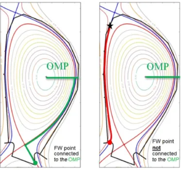
It is important to model the wall surface geometry using a fine mesh and determine if particles can hit each loca-tion. A backward calculation is more convenient in this case, allowing one to calculate whether each area element in the wall surface is magnetically shadowed or not. The principle of the magnetic shadowing calculation is to start from any location of the first wall and to follow the mag-netic field line (thus at constant magmag-netic flux ψ) in the backward direction.
• If this magnetic field line reaches the OMP first, the specified location of the FW can receive particles from the OMP and thus charged particle heat load (shad-owing S = 1).
• If the magnetic field line is intersected by an object before reaching the OMP, the specified location of the
FW is magnetically shadowed and can’t receive heat load (shadowing S = 0).
Fig. 1 gives a 2D representation of the magnetic shad-owing calculation, with, on the left a point of the FW from which the field line reaches the OMP, and on the right an-other point of the FW from which the field line intersects a wall. These figures are 2D representations for better understanding but PFCFlux calculations are done in 3D.
Figure 1: Maps of magnetic fluxes with a representation of the mag-netic shadowing calculation of PFCFlux
2.2. Heat load calculation
In the so-called ”far-SOL” the parallel heat flux con-ducted by the particles decreases exponentially as func-tion of a decay length λq (from 6mm to 50mm in function
of the equilibrium considered [1]). The parallel flux at a given position on the OMP is given in equation (1)
φ(d) = φ0× e−d/λq (1)
where d is the geometric distance at the OMP between the LCFS and the magnetic field line at given magnetic flux ψ. The maximum parallel heat flux value φ0 is fixed
so that the integration of the parallel heat flux over the OMP matches the total power conducted by the particles through the SOL.
Z
OM P
φdS = Pcond (2)
A link between the geometric position and the magnetic flux at the OMP can be done, giving for the parallel heat flux :
φd(d) = φψ(ψd) (3)
Figure 2: Heat load on a limiter for different number of limiters
with ψdthe magnetic flux of a magnetic field line at the
OMP, at a distance d from the LCFS. φψ is the
paral-lel conductive power written in function of the magnetic flux. From now, φ(d) and φ(ψd) are used to describe the
parallel heat flux at the OMP, in function of the distance to the LCFS or the magnetic flux, in their corresponding formulation.
The heat load on the wall ϕ, at a position ~r and with a magnetic flux ψ is calculated by the following equation:
ϕ(~r, ψ) = φ(ψ) × sin(α(~r)) × fx(~r) × S(~r) (4)
where α(~r) is the incident angle of the magnetic field line on the wall at the position ~r, fx(~r) is the magnetic
expansion of the field line between the OMP and the position ~r, and S(~r) is the result of the shadowing calculation (see part 2.1).
2.3. Power ratio ρ
After each PFCFlux calculation, a power ratio ρ is cal-culated between the integral of the heat flux on the walls (including the divertor) and the total power conducted through the SOL.
ρ = R wallϕdS R OM PφdS (5) In most cases, a point on the wall is paired with exactly one point on the OMP within one poloidal turn, leading to a power ratio ρ close to 1, ensuring good energy conser-vation.
However, in limited equilibria using discrete limiters in 3D, this power ratio drops down as far as 0.2, i.e. only 20% of the power conducted by the particles is distributed on the wall. Figure 2 shows the heat load on a DEMO limiter for different numbers of limiters (4, 8 and 16). For these three backward calculations, the power ratio ρ increases 2
from 0.29 with 4 limiters to 0.51 with 8 limiters and 0.8 with 16 limiters.
One can see that for the cases with 4 and 8 limiters, the wetted area given by the backward shadowing calculation is almost identical.
As the magnetic flux ψ is assumed to be toroidally con-stant, the heat flux calculation on a limiter gives the same result in the 4 limiters case as in the 8 limiters case.
Thus, with the same wetted area and heat flux pattern for these two cases, this explains why the power ratio is almost two times lower in the 4 limiters case than in the 8 limiters case.
The missing power is explained by the fact that some points from the OMP are not directly paired with the wall and need more than one poloidal turn. The backward cal-culation fails to account for all the points from the OMP connected to the same point on the wall. Thus, wall heat fluxes are underestimated and rescaling is needed to give heat flux values consistent with energy conservation.
3. Modeling of the missing power 3.1. Case studied
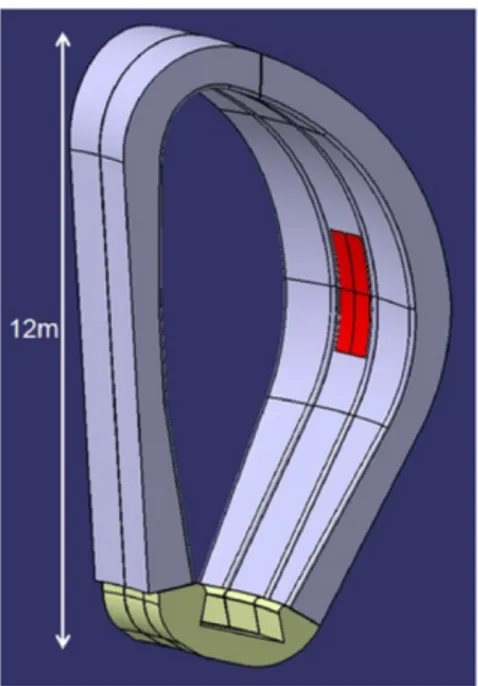
To understand the missing power in the previous case, a forward calculation is performed from the OMP. For each location on the OMP, we follow the magnetic field lines in the forward direction and see if this line hits a wall, a limiter, or the OMP itself. Calculation was done with PFCFlux on the CAD geometry of DEMO (see Fig-ure 3): 16 sectors of FW (height = 12m, minor radius = 6m, major radius = 12m) and 2-16 equatorial outer limiters (height=2.8m,width=1.1m, maximum protrusion to FW = 2cm) . A magnetic equilibrium corresponding to a plasma current ramp-up case (Fig. 4), where the power conducted by the particles Pcond=6MW and the
decay length λq=6mm, based on the DEMO prediction in
[1].
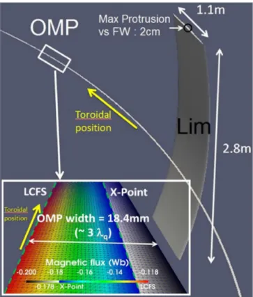
The most representative part of the OMP was mod-eled (range of magnetic flux from the value at the LCFS (ψLCF S) to a value slightly greater than that at the
X-point (ψX), representing an OMP width of 18.4mm, see
the small black rectangle on Fig.4 and see Fig. 5).
3.2. Area of missing power
The aim of this calculation is to detect the area where the OMP is paired with a wall or limiter and where the OMP is connected to itself (leading to missing power in the backward calculation). The results shown in Figure 6 illustrate a small area of the OMP (see rectangle in figure 4) for calculations with 2, 4, 8 and 16 limiters.
In these figures, the green area represents all points from the OMP directly connected to the wall or to the lower divertor, as expected since these points have a magnetic flux ψ < ψX (so from white to black on figure 4). As these
magnetic flux surfaces are open (see figure 5), a field line
Figure 3: CAD geometry of a sector (22.5◦) of DEMO - FW in blue - Outer limiter in red - Lower divertor in yellow
Figure 4: Map of magnetic flux : plasma current ramp-up equilib-rium. Ip=6MA. Bold red line : X-Point. Bold green line : LCFS.
Figure 5: Outer mid plane modeled in front of an outer limiter. Magnetic flux on the OMP from the LCFS to a little further than X-Point magnetic flux.
from a point on the wall cannot perform more than one poloidal turn before touching another wall.
The red area indicates all points from the OMP not paired with the wall or the limiters. A field line can com-plete a full poloidal turn without touching the FW or a limiter, and thus this represents the missing power in a backward calculation.
The white areas show the link between the OMP and a limiter: the areas from which particles can leave the OMP to hit a limiter.
One can see that when there are fewer limiters the red area is larger, explaining why the power ratio ρ during backward calculation decreases with the number of lim-iters.
This figure presents a local area of the OMP (at one toroidal position) but the result is not toroidally symmet-ric. For another toroidal position, the locations of white and red areas are different due to the position of the lim-iters, and can be larger or smaller. Actually, the connected areas depend on the distance to the limiters. The magnetic flux where the OMP is connected to a limiter is thus not constant toroidally.
3.3. Quantification of the missing power
For each value of magnetic flux on the OMP, we compare the area of the OMP connected to an object to the area connected to the OMP itself. This is thus the toroidal mean of the result illustrated in figure 6. This operation
was carried out for each limiter configuration (2 limiters to 16 limiters). Results are presented in figure 7.
One can notice that the missing power is not equally dis-tributed. The missing power is mostly concentrated near the LCFS, while it is negligible beyond ψX. For ψ < ψX,
the divertor and FW are concerned by the heat load and therefore the issue with discrete object disappears. There is thus no obvious reason to change heat flux value for ob-jects whose ψ < ψX. On the other hand, for objects whose
magnetic flux ψ is close to ψLCF S, the heat load is
prob-ably underestimated by a large fraction, as the missing power may be up to 95% of the expected power.
Figure 8 represents the effective heat flux profiles used at the OMP for different number of limiters inside the tokamak. The original profile is given by the red curve, but because of the missing power illustrated in figure 7, the effective profile obtained for the different cases is not an exponential decay anymore. The area ratio between a given curve and the expected one (red curve) represents the power ratio for this forward calculation. These ratios (ρ in the legend) are very close to the ones observed after a backward calculation (see 2.3), meaning that the same phenomenon occurs in forward and backward calculations.
4. Rescaling of heat load calculations with missing power
4.1. Basic rescale
The easiest way to rescale the missing power is to divide the heat load on the wall by the power ratio ρ.
ϕbasic rescale= ϕ × R OM PφdS R wallϕdS (6)
This method implies that the missing power is equally distributed on the FW and limiters, but Fig. 7 shows that this is not the case and this approach is surely not acceptable. With this rescaling, the heat flux profile at the OMP is no longer exponential.
4.2. Rescaling for each ψ value
A second way to rescale the heat load is to quantify the missing power at the OMP for each distance to the LCFS.
ϕψ rescale(d) = ϕ(d) × R OM PφdS d R wallϕdS d (7)
The main hypothesis is that different spots on the walls or limiters with the same magnetic flux receive the same missing power. The validity of this method is also ques-tionable because of the toroidal asymmetry of the geome-try.
Figure 6: Result of a field line tracing from the Outer Mid Plane for different number of limiters Green : the OMP is connected to a wall -White : the OMP is connected to a limiter - Red : the OMP is not paired with the wall/limiters (connected to itself)
Figure 7: Percentage of missing power at the OMP. LCFS is at x=0. λq= 6mm. P = 6M W .
Figure 8: Effective heat flux profile used on the OMP due to the missing power issue. λq= 6mm. P = 6M W .
Figure 9: Simplified representation of a magnetic field line starting from a limiter and hitting two positions of the OMP (red dots) before hitting another limiter
4.3. Rescaling as a function of the maximum number of poloidal turns
This third method relies on the fact that the mapping between the OMP and the wall is not bijective but sur-jective. To find all OMP points associated to a given wall point, the algorithm needs to continue following the field line even after reaching the OMP, until it hits another ob-ject. The number of particles coming from different points of the OMP to the same location of an object is then equal to the number of poloidal turns made (see Fig. 9).
4.4. Effect of the different rescaling methods on the heat load on limiters
The different rescaling methods have been tested on a 4-limiter case. Fig. 10 shows the heat load on the front face of a limiter, after rescaling using the different methods presented above.
When no rescale is done, the ratio of power recovered is about ρ = 0.29, with a maximum heat flux of 1.03M W/m2
on the limiter. The basic rescale doesn’t modify the dis-tribution of the heat load on the limiter, but just forces the power ratio ρ = 1 after rescaling. This method gives a maximum heat load of 1.03/ρ = 3.54M W/m2.
Figure 10: Heat load on a limiter for the different rescaling methods.
The second method (rescaling for each ψ value) increases the heat load on the center of the limiter, which has the highest value of ψ and thus has the greatest missing power according to Fig. 7. The maximum heat load in this case increases to 8.2M W/m2.
Rescaling by the number of passes through the OMP presents a more intriguing pattern, with very high heat load localized at some values of ψ, reaching 21.7M W/m2.
These areas are positioned where the ratio of toroidal turns to poloidal turns is almost rational, giving very little toroidal movement of the intersection point with the OMP, and thus needing many poloidal turns before reaching an-other wall. The magnetic field lines have been followed to a distance of up to 7km.
5. Conclusion and prospects
Simplified models using 3D field line tracing are used to design the shaping of the PFCs in new tokamaks. These models allow fast simulations for optimizing the design of the FW and limiters. Limiter equilibria are difficult to model accurately with this approach, because it leads to some missing power, due to the fact that the mapping from the OMP to the FW becomes surjective instead of bijective. Several methods were discussed to rescale the heat load on limiters and FW to match the power balance. The rescaling is of importance since the resulting heat load on the limiter is multiplied by a factor of 3-21.
Comparison with experiments and simulations carried with more physical realism would help to understand and quantify the errors of each rescaling method and improve the rescaling method. In particular the method based on the number of passes through the OMP could be improved by including cross-field transport, which is clearly needed for high connection length.
Acknowledgments
This work has been carried out within the framework of the EUROfusion Consortium and has received funding
from the Euratom research and training programme 2014-2018 under grant agreement No 633053. The views and opinions expressed herein do not necessarily reflect those of the European Commission.
References References
[1] R. Wenninger et al. The DEMO wall load challenge. Nucl. Fu-sion, 57 (046002), 2017.
[2] F. Maviglia et al. Wall protection strategies for DEMO plasma transients. Fusion Eng. Des., 136:410–414, 2018.
[3] P.C. Stangeby. A three-dimensional analytic model for discrete limiters in ITER. Nucl. Fusion, 50 (035013), 2010.
[4] M. Firdaouss et al. Modelling of power deposition on the JET ITER like wall using the code PFCFlux. Journal of Nuclear Materials, 438:536–539, 2013.
[5] W. Arter et al. The SMARDDA approach to ray tracing and par-ticle tracking. IEEE Trans. Plasma Sci, 43-9:3323–3331, 2015.