HAL Id: hal-01384319
https://hal.archives-ouvertes.fr/hal-01384319v2
Submitted on 21 Oct 2016
HAL is a multi-disciplinary open access archive for the deposit and dissemination of sci-entific research documents, whether they are pub-lished or not. The documents may come from teaching and research institutions in France or abroad, or from public or private research centers.
L’archive ouverte pluridisciplinaire HAL, est destinée au dépôt et à la diffusion de documents scientifiques de niveau recherche, publiés ou non, émanant des établissements d’enseignement et de recherche français ou étrangers, des laboratoires publics ou privés.
bacteria perform as fast as ostriches?
Nicole Meyer-Vernet, Jean-Pierre Rospars
To cite this version:
Nicole Meyer-Vernet, Jean-Pierre Rospars. Maximum relative speeds of living organisms: why do bacteria perform as fast as ostriches?. Physical Biology, Institute of Physics: Hybrid Open Access, 2016, 13 (6), pp.1-13. �10.1088/1478-3975/13/6/066006�. �hal-01384319v2�
do bacteria perform as fast as ostriches?
Nicole Meyer-Vernet1 and Jean-Pierre Rospars2
1LESIA, Observatoire de Paris, CNRS, PSL Research University, Sorbonne Univ.,
UPMC, Univ. Paris Diderot, Sorbonne Paris Cit´e, 92195 Meudon, France
2Institut National de la Recherche Agronomique (INRA), UMR 1392, Institut
d’Ecologie et des Sciences de l’Environnement de Paris, 78000 Versailles, France E-mail: nicole.meyer@obspm.fr
Abstract.
Self-locomotion is central to animal behaviour and survival. It is generally analysed by focusing on preferred speeds and gaits under particular biological and physical constraints. In the present paper we focus instead on the maximum speed and we study its order-of-magnitude scaling with body size, from bacteria to the largest terrestrial and aquatic organisms. Using data for about 460 species of various taxonomic groups, we find a maximum relative speed of the order of magnitude of ten body lengths per second over a 1020-fold mass range of running and swimming animals. This result
implies a locomotor time scale of the order of one tenth of second, virtually independent on body size, anatomy and locomotion style, whose ubiquity requires an explanation building on basic properties of motile organisms. From first-principle estimates, we relate this generic time scale to other basic biological properties, using in particular the recent generalisation of the muscle specific tension to molecular motors. Finally, we go a step further by relating this time scale to still more basic quantities, as environmental conditions at Earth in addition to fundamental physical and chemical constants.
Keywords: biological scaling, locomotion, molecular motors, metabolic energy, Earth-based life
1. Introduction
Autonomous locomotion is a fundamental property of animals, which involves an amazing diversity of mechanisms and has important consequences for ecosystems and evolution [1]. Biological scaling generally focuses on the preferred speed V , which minimizes the power or maximises the range and is primarily determined by dynamical constraints [2–5]. Because of the major role played by the gravitational acceleration g, most scalings with size L can be related to the ratio of kinetic to gravitational energy - the so-called Froude number F r = V2/Lg. For animals sharing similar locomotor mechanisms, this yields V ∝ (Lg)1/2 ∝ M1/6g1/2 if the body mass M ∝ L3 [6, 7].
The present study focuses instead on the maximum speed reached by animals when they are driven by circumstances to move faster than their natural speed, as for catching preys or escaping. Although such a speed has different consequences on behaviour from the preferred speed, it may be central to survival. Various scalings have been found over relatively narrow mass ranges or restricted animal groups and gaits, with allometries often compatible with a constant ratio of kinetic to gravitational energy, albeit with a value of F r variable and higher than for the preferred speed [8–12]. However, on a very large scale and in order of magnitude, the maximum speed has been shown by Bonner [2, 13] to be roughly proportional to body length L over nearly the 1020-fold mass range of running and swimming organisms - a fundamental and unexplained property which generalises a result observed for fishes [14–16]. If most aquatic and terrestrial species have a similar maximum relative speed Vmax/L, this implies a locomotor time scale (L/Vmax), whose near independence on size contrasts with the general increase of physiological time scales with body mass - smaller animals having a faster pace of life [17]. Furthermore such a ubiquitous time scale - holding from bacteria to large fishes and from small mites to ostriches, requires an order-of-magnitude explanation ignoring details and based on first principles. To the best of our knowledge, this has not been previously analysed nor interpreted in the biological literature.
Interpretations should build on basic properties common to motile organisms. Chemistry yields a huge range of time scales because of the variations in reaction rates with concentration, temperature, and catalyst. The next structural level is that of proteins, whose folding time scales span a large range, from about 10−4 to 102 s for typical numbers of amino-acids N ∼ 102− 103 [18]. A larger scale is the cell size, close to 10 µm for most organisms [19], so that the diffusion time scale of proteins in cells is 10−3− 10 s [20]; however in the cellular complex structure, diffusion is expected to be strongly modified and overwhelmed by non-thermal processes such as active transport mediated by molecular motors [19]. A different viewpoint is to consider macroscopic biological quantities which may limit the relative speed - the mass density, the specific tension of biological motors [22], and the maximum specific metabolic rate [23], as proposed by Meyer-Vernet and Rospars [24] using dimensional analysis in a preliminary paper written in the context of physics teaching.
(supplementing, analysing and referencing the preliminary set plotted in Ref [24]) to deduce the maximum speed as a function of body’s mass and the resulting time scale. Section 3 deals with an interpretation. Since the result is approximate and nearly independent on size and locomotion style, holding both from bacteria to large fishes and for all running taxa, we make first-principle order-of-magnitude estimates. We build in particular on the universality of the specific tension [22] used by organisms for their locomotion (section 3.1), based on a recent generalisation of the muscle tension to molecular motors [21, 22]. Section 4 examines the compatibility of the results with other empirical scalings, and tries to relate them to more basic properties. Indeed, from the physicist’s perspective, proposing to explain the order of magnitude of a time scale from known biological quantities as in a Fermi’s problem is not sufficient, unless we are able to calculate these biological quantities themselves from basic numbers. Since the organisms studied evolved on Earth, these basic numbers are expected to involve environmental conditions at Earth, in addition to fundamental physical or chemical constants. In particular, as Feynman once said [25], “all the things that we see that are moving, are moving because the sun is shining”; so, can we relate this scale to the amount of solar energy reaching Earth?
2. Methods and empirical results
Values of the maximum speed as a function of mass were taken from tables of values published in the literature listed in subsection 2.3 for a variety of running or swimming animals of different taxonomic groups, ranging in mass from an eubacteria (M ' 2 × 10⁻¹⁶ kg ) to the blue whale (M ' 1.5 × 10⁵ kg).
We only consider the velocity of organisms as a whole (i.e. the speed of the centre of mass). Hence, we include neither plants and fungi nor sessile animals. We do not consider either the motions resulting from sudden release of stored elastic energy as fleas’ jumps or spasmoneme motion [26], nor motion on inclined supports, or adhesive locomotion used for example by gastropods [27] and pili [28], nor cells’ crawling [29], which is based on a completely different mechanism from that considered here [30]. For microorganisms, we select the data for which the recorded speed cannot be confused with diffusion resulting from random directional changes, or with a drift due to gravity or chemical gradients [31].
In order to study the relative speed as a function of mass, we need empirical values of the three quantities Vmax, M and L. They are determined as follows.
2.1. Maximum speed
How is the empirical “maximum speed” defined? Does it mean a maximum speed sustainable for long periods, or a top speed briefly attainable in a sprint? The top speed requires the additional contribution of transient (anaerobic) processes leading to fatigue, whereas animals in prolonged (aerobic) locomotion must achieve oxygen balance, so that
the speed at which the maximal rate of oxygen consumption is attained is usually called the maximum aerobic speed.
Most data on mammals concern the transient maximum (top) speed, which has been found to be in average 2-3 times higher than the maximum sustainable speed [8, 32]. For ectothermic species, which typically move in short bursts of exercise followed by periods of recovery, most recorded data concern the “burst” speed, expected to be close to the top speed. For fishes, the average top speed (called “escape” speed) is known to be 3–4 times greater than the average sustained speed [15, 35]. This order-of-magnitude similarity of the transient top speed and the maximum sustained speed is in line with the observed similarity in order of magnitude of the maximum anaerobic (transient) and aerobic (sustainable) metabolisms [36] (see section 3.2). Since we seek order-of-magnitude values over a wide range of species and masses, we therefore consider the top speed, which represents the majority of the available maximum speed data.
Note that since both original and secondary sources were consulted, with experimental conditions not always available, the results may not be homogeneous in this respect. Indeed, the motivation to run and swim as fast as possible depends on the species and the experimental procedure; convincing a mite or an ostrich to run fast does not require the same tools. Therefore, since the diversity of animal sizes and gaits necessarily produces large differences in experimental set-ups, the data have variable degrees of accuracy - a problem inherent to considering organisms over a 20-fold mass range.
Another question concerns the temperature, which affects reaction rates and therefore speed. As far as possible, we selected the data corresponding to the mean body temperature of animals active in the field. For ectothermic organisms, the range of such temperatures is expected to produce a significant range in speeds; we shall discuss this point in section 4.3. We did not make corrections for the sake of consistency, because no such corrections were applied neither for deducing the constancy of the specific tension nor the constancy of the maximum specific metabolism (see e.g. discussion in Ref. [23]), which are used in our interpretation.
Similarly, we did not correct either for the phylogenetic context [33, 34]. Although phylogenetic considerations might affect the regressions (see e.g. [37, 38]), they should not invalidate our main result that the motional time scale has the same order of magnitude over the entire mass range.
2.2. Mass and length
When only one of the two parameters M and L was available we determined the other one from the documented relation between them. Since organisms of different sizes must compensate for varying dynamical and physiological conditions, they cannot be precisely geometrically similar. As size increases - implying larger dynamic forces, whereas the elasticity of materials remains constant, the length-to-diameter ratio L/D may have to decrease in order to prevent excessive deformations, yielding the relation D2 ∝ L3,
whence M ∝ L4 [2, 39]; this so-called elastic similarity holds for some properties in limited size ranges [2]. Another relevant constraint is the resistance of tendons and skeletons, which leads to stress similarity within some taxa [40]. However, recent observations show that for large-scale variations expressed in order of magnitude - which is what is needed here - geometric similarity is generally more adequate, i.e. M ∝ ρL3, ρ being the mass density, with a constant of proportionality depending on shape as summarized below.
First, for all terrestrial non-flying mammals, mass and length can be approximated by M ' (3L)3 (in SI units) over most of their size range [41] (although elastic similarity tends to hold for very large mammals [42]). By comparing with empirical allometries holding for various taxa [12, 43, 44], we have verified that extending this relation to non-mammals produces errors that do not affect significantly the results. An exception is the case of very elongated species as snakes and worms; hence we did not include limbless terrestrial taxa; we shall return to this point in section 4.2.
Second, swimming species (except microorganisms) tend to have a stream-lined shape with M ' (2L)3 (in SI units) [45].
Third, motile microorganisms have a much greater diversity of shapes (with a median at L/D ' 3) [16, 46, 47], the elongation being expected to facilitate their orientation by increasing the resistance to rotation induced by Brownian motion [16]; because of this diversity, we keep only microorganism data for which both L and M or L and D are available (contrary to the preliminary data plotted in Ref. [24]). When only L and D are available, we estimate M using the prolate spheroid approximation M = (π/6)ρL3(D/L)2. For our microorganism data set, the mean of L/D ' 4.8 (M ' (1.6L)3) with a standard deviation ' 6.4 and a median of 2.4 (M ' (3.3L)3).
2.3. Maximum speed versus body mass
Figure 1 shows the measured maximum (top) speed as a function of mass for about 460 species of different taxonomic groups. The data for 155 terrestrial mammal species (taken from [9] plus some species from [8, 48] not included in [9]) are plotted in magenta. The data for 137 other running species (a set roughly three times larger than considered in Ref. [24]) are plotted in green. They include 14 ant species [2, 11, 49], 16 other arthropod species (including crabs [50], mites [2,51], spiders [52,53], cockroaches [54] and beetles [55]), 100 species and subspecies of lizards [12], and 7 species of terrestrial birds [56–60]. This yields a terrestrial mass range spanning nearly 12 orders of magnitude, from 10−8 kg (clover mite) to 6000 kg (African bush elephant). The maximum speeds for 95 swimming mites, fishes, cetaceans, crustaceans, penguins, turtles, and squids [2, 5, 14, 15, 61–67] and 71 microorganisms [2, 46, 68–70] are also plotted (in blue). This yields a 7 × 10²⁰-fold range in mass, from 2 × 10⁻¹⁶kg (eubacteria) to 1.5 × 10⁵ kg (blue whale).
We have superimposed (dashed) regression lines of log10Vmax versus log10M in magenta for running mammals (slope 0.16 with 95% confidence limits (CL) [0.14, 0.18],
10−16 10−14 10−12 10−10 10−8 10−6 10−4 10−2 100 102 104 106 10−6 10−4 10−2 100 102 body mass (kg) maximum speed (m/s) Terrestrial mammals Terrestrial non−mammals Aquatic species
Figure 1. Maximum speed versus body mass for terrestrial mammals (in magenta) and non-mammals (in green), and aquatic species (in blue) from the references cited. The corresponding regression lines are shown (dashed) in similar colors, and the
regression line for all data is shown in (dashed) black. Maximum running and
swimming speed (black solid line, equation (7)) and upper limit at large masses (dotted) are also shown as estimated in section 3.
intercept 0.83, correlation coefficient r=0.80, n = 155), green for running non-mammals (slope 0.35 with 95% CL [0.31, 0.38], intercept 0.87, r=0.88, n = 137), and blue for swimming (slope 0.34 with 95% CL [0.33, 0.36], intercept 0.48, r=0.98, n = 166). The regression line for all running and swimming data is plotted in (dashed) black (slope 0.35 with 95% CL [0.34, 0.36], intercept 0.70, r=0.97, n = 458). In all data subsets the slope of the regression line is highly significantly different from 0 (P < 10−3). The proportion of the total variance explained by the regression is 64% for running mammals, 77% for running non-mammals, 96% for swimmers and 94% for swimmers and runners together. Figure 1 also shows that the maximum speed tends to level-off for large organisms, which confirms a known result [2, 8, 9] and strongly affects the fitted exponent of terrestrial mammals which includes a high number of large animals; we shall return to this point later.
2.4. Maximum relative speed and corresponding time scale
In figure 2 the time scale τ = L/Vmax is plotted as a function of body mass for the organisms considered in subsection 2.3. The slope of the regression line of log10τ versus log10M for all data, plotted as a dashed line (slope -0.008 with 95% CL [−0.017, 5×10⁻⁴], intercept -1.127, r = 0.087, n = 458) is not significantly different from 0 (P = 0.06). Terrestrial species have a mean ' 0.082 s (SD ' 0.10 s, median ' 0.049 s, n = 292), close to that of mammals only (0.091 s). Swimming species have a mean ' 0.27 s (SD ' 0.49 s, median ' 0.12 s, n = 166). Note that microorganisms (M . 10−8 kg, mean ' 0.37 s, SD ' 0.66) and other swimmers (M & 10−8 kg, mean ' 0.20 s, SD ' 0.28) have similar medians (' 0.12 s) and similar logarithmic means (' 0.14 s) despite the
10−16 10−14 10−12 10−10 10−8 10−6 10−4 10−2 100 102 104 106 10−3 10−2 10−1 100 101 body mass (kg)
Locomotor time scale (s)
Terrestrial mammals
Terrestrial non−mammals
Aquatic species
Figure 2. Locomotor time scale as a function of body mass for terrestrial mammals (in magenta) and non-mammals (in green), and aquatic species (in blue) from the references cited in subsection 2.3. The dashed line τ = 10−1.127 × M−0.008 is the
regression of log10τ versus log10M for the whole data set. The solid line (with values
smaller and larger by one order of magnitude dotted) is from (6), estimated in section 3; the limit for large masses estimated in subsection 3.4 is shown dash-dotted. For clarity the scale is twice larger on the speed axis than on the mass axis.
huge difference in mass. The larger variability of microorganism data may result in part from the increased difficulty in measurement of both size and speed as size decreases. The mean of all data together is ' 0.15 s (SD ' 0.3 s, median ' 0.07 s). More than 98% of the data lie in the range 10−2 < τ < 1 s, which is remarkably narrow compared to the 1020-fold variation in body mass. The next section proposes an order-of-magnitude interpretation of these empirical results.
3. Physical interpretations
The locomotor time scale of living organisms is expected to depend on at least three basic macroscopic properties, whatever their size and locomotion style: their mass density ρ, which is close to that of water
ρ ' 103 kg m−3 (1)
the maximum force per cross-section area σ (specific tension) that they can exert, and the maximum power per mass unit bM (maximum specific metabolic rate) that they can use for moving. Let us consider in turn the two latter factors.
3.1. Specific tension
The force per cross-sectional area of skeletal muscles at constant length (the so-called isometric specific tension) is known to be remarkably constant whatever the muscle and body mass, because of the similar construction of skeletal muscles based on the myosin molecule [71, 72]. This notion of specific tension has been formally generalised
to individual molecules [21, 22] and to propulsion organelles and individual molecular motors propelling microorganisms [22], showing that their maximum specific tension has a similar statistical distribution as that of conventional muscles, and that the maximum applied force per unit cross-section area is about
σ ∼ 2 × 10⁵ N m−2 (2)
over about 19 orders of magnitude in body mass, from microorganisms to the largest animals [22]. 0 500 1000 1500 σ (kPa) 0 20 40 60 80 100 Cumulated number (%) Non-locLoc n = 55 260 µ = 5.20 5.09 SD = 0.92 0.62 P = 0.07 0.02 A 0 50 100 150 200 250 300 350 σ < 350 kPa 0 20 40 60 80 100 Cumulated number (%) Non-loc Loc n = 44 243 µ = 143 173 SD = 60 77 P = 0.96 0.34 B
Figure 3. Empirical cumulative distribution functions (CDFs) of the specific tension σ used for locomotion (red) and other functions (blue) in aquatic and terrestrial species. Panel A shows empirical CDFs of all σ values (solid) fitted to lognormal CDFs of mean µ and SD indicated (dotted). Panel B shows empirical CDFs of values σ < 3.5 × 10⁵
Pa fitted to Gaussians (dotted) of mean and SD indicated. CDFs of locomotors
and non-locomotors are not significantly different at level 5% (P = 0.13) in A and significantly different (P = 0.01) in B. All comparisons based on Kolmogorov-Smirnov tests. (References of the data in Rospars and Meyer-Vernet [22]).
.
We are interested here in the specific tension used for locomotion. Figure 3 compares the cumulative distributions of the values of σ used (in red) or not (in blue) for locomotion. The values smaller than 3.5 × 10⁵ Pa (corresponding to the inflection point of the distributions in figure 3A), which can be fitted to Gaussians, are plotted in the right-hand-side panel.
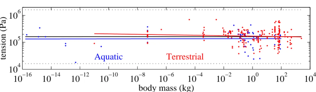
Figure 4 shows the specific tension used for locomotion as a function of cell or body mass for 260 terrestrial and aquatic species. The slope of the regression lines (-0.008 with 95% CL [-0.022, 0.005], n = 207, P = 0.22 for terrestrial species, 0.0008 with 95% CL [-0.017, 0.018], n = 53, P = 0.93, for aquatic species) and 6 × 10⁻⁵ with 95% CL [-0.0096, 0.0097], n = 260, P = 0.99 for all data together) are not significantly different from 0. The mean of all values of σ is 1.84 × 10⁵ (SD 1.1 × 10⁵, median 1.74 × 10⁵) N m−2.
The order of magnitude of this ubiquitous value of σ can be interpreted from first principles. Molecular motors as the myosin molecule [73] move by steps via a conformational change of their 3-D structure, so that the elementary step length is of the order of magnitude of their size, which is the typical protein size a0 ∼ 6 nm
10
−1610
−1410
−1210
−1010
−810
−610
−410
−210
010
210
410
410
510
6body mass (kg)
tension (Pa)
Aquatic
Terrestrial
Figure 4. Specific tension used for locomotion versus cell or body mass for terrestrial (in red) and aquatic (in blue) species, and corresponding log-log regression lines, with the regression for all data plotted in black (σ = 105.21× M0.00). The dotted lines
are the values smaller and larger by one order of magnitude. For clarity the scale is about twice larger on the tension axis than on the mass axis. (References of the data in Rospars and Meyer-Vernet [22]).
.
[74]. Each such step is mainly powered by the ATP release energy, of standard value W0 ' 0.5 × 10⁻¹⁹ J per molecule, so that the elementary force exerted by the motor is F0 ∼ W0/a0 in order of magnitude [75], whence the force per unit motor’s cross-section [22]
σ ∼ W0/a30 (3)
Substituting the above values of W0 and a0 into (3) yields (2).
3.2. Mass-specific metabolic rate
Most analyses of the energy consumption rate B of living organisms concern the so-called “basal” (“resting”) or “field” metabolic rates, depending on whether the organism is at rest or is performing its normal tasks. To compare organisms of different body mass M , it is convenient to define the mass-specific metabolic rate b = B/M . Power laws of the form b = αMβ have been fitted to various sets of data, yielding various scaling exponents, and fostering an amazing variety of models [76]. Since exchanges with the environment act through surfaces (∝ M2/3, yielding b ∝ M−1/3 - although such surfaces may scale differently [77, 78]), whereas internal resources vary with volume (∝ M , yielding b ∝ M0), one may expect −1/3 < β < 0, depending on the relative importance of external and internal constraints [79], if other properties as the transport system co-adjust [80]. This range covers most of the observations, including the so-called Kleiber’s law exponent β = −1/4 which remains controversial [17, 38] and in particular has been found not to hold for prokaryotes and protists [82]. Recently, b has been found to be constant in order of magnitude across the 1020-fold mass range of living organisms in comparable physiological states at natural temperatures [81] - a result compatible with the variety of exponents β because of the variation of the intercepts α for different taxa and mass ranges.
An important point is that the exponent β varies with the physiological state of the organisms, approaching zero at high level of activity [79, 84], which is the relevant state at maximum speed. Indeed, at high activity, the metabolism is expected to be mainly determined by the resource demand of working tissues, which scales as their mass (∝ M ), as does the oxygen and energy stored which are used during bursts of maximal activity. Hence the maximal specific metabolic rate is expected to be roughly constant in order of magnitude - at least when normalized to the mass of active tissues, as observed [23, 83–85].
This maximal specific metabolic rate bM, ubiquitous in order of magnitude across the 1020-fold mass range of living organisms, may represent a biochemical limit universal for life; measurements on dividing bacteria and moving animals during peak activities yield the maximal value
bM ∼ 2 × 10³ W kg−1 (4)
per unit mass of active tissue [23], like the mitochondria [84, 86–88] at their natural temperature. For example in mammals, over 90% of the energy at maximum metabolic rate is consumed in locomotor muscles, which are densely populated of mitochondria -the energy factories of eukaryotic cells - and we have bM ' 1600 W/kg of mitochondria mass [83, 84]. The value per unit body mass is smaller by the proportion of active tissue in the body (typically 1-50%), and is typically 5-30 times higher than the resting specific metabolic rate b for both vertebrates [1] and invertebrates [89]. In particular, the maximum metabolic rate per unit body mass amounts to only about 90 and 100 W/kg body mass for respectively (20 g) European woodmouses (Apodemus sylvaticus) and (28 kg) pronghorns (Antilocapra americana) [83], whose bodies have a large proportion of mitochondria, whereas it amounts to only about 20 W/kg body mass for human [36] and insect [89] runners.
Most of these measurements concern the aerobic metabolism, measured via oxygen consumption. At (short term) peak activity, part of the energy - or even most of it for ectoterms, is supplied by transient anaerobic processes [90]. However, the total maximal energy output is found to be generally similar in order of magnitude [36], the smaller aerobic power of ectoterms being compensated by a larger anaerobic power (e.g. [91–93]).
3.3. Consequences on the locomotor time scale
A basic order-of-magnitude estimate of the locomotor time scale can be derived from the constraints addressed above. Consider first a micro-organism whose locomotion is powered by N molecular motors of size a0, making it move by about its length L at the frequency f so that its speed is V ' Lf . Assuming that each motor (of mass ρa3
0) uses the elementary energy W0 for each such step, the total power is N W0f , which cannot exceed the maximum value N ρa30 × bM. This yields fmax ∼ ρa30bM/W0 [24], whence τ ∼ W0/(ρa30bM). From the expression (3) of σ we deduce
Substituting (1), (2) and (4) into (5) yields
τ = L/Vmax∼ 0.1 s (6)
Consider now an animal of length L, cross-section S⊥, and mass M ∼ ρS⊥L, moving via cyclic (of frequency f ) motion of appendages such as runners’ legs or fishes’ tail and fins. For an appendage i of length Li, muscle section Si, and tension σi rotating by θi with a lever arm li, the work performed is Wi = Γiθi with the torque Γi ∼ σiSili, so that the total work of the appendages is W ∼ ΣiσiθiSili. With the approximations θi ∼ 1 radian, σi ∼ σ, L ∼ Li ∼ li and S⊥ ∼ ΣiSi, the specific work per cycle is thus W/M ∼ σ/ρ - a gross simplification which also neglects the role of elastic elements and of gears and joints, and assumes that the applied tension is the maximal one, despite the actual variation of tension with muscle speed. If the step size is approximated by L, and both the efficiency and the proportion of muscle and active tissue are approximated by 100%, the specific power is therefore σf /ρ, which cannot exceed bM. This yields the time scale (5), i.e. (6), which is drawn as a solid black line on figure 2.
Substituting into (6) the average relation M ' (2.8L)3 deduced from the (logarithmic) average of M/L3 for the plotted data, we find the maximum speed
Vmax∼ 3.5 M1/3 (7)
which is drawn as a solid black line in figure 1 and is very close to the experimental dashed black line.
It may seem surprising that these order-of-magnitude estimates, which are little more than dimensional analysis estimates and make so drastic assumptions as to the actual mechanisms of locomotion [4, 86] agree with observation. It appears that the large number of factors that have been approximated by unity turn out to compensate each other in order of magnitude.
3.4. Upper limit to the maximum speed
Figure 1 suggests that the speed reaches a maximum value ∼ 15 m/s for masses exceeding ∼ 50 kg (L ' 1.5 m), which confirms known results [2, 8, 9]. Since this upper limit holds for both running and swimming (with a Reynolds number Re varying from 10−5 for bacteria to more than 108 for large fishes), it is not expected to result from constraints related to the locomotion style [40, 94] or to the drag, which depend on the ambient density and on Re. Such a ubiquitous constraint may derive instead from an argument inspired by Hill [95]. Consider again the periodic motion of an appendage of length Li and mass Mi ∼ ρSiLi. This motion is expected to be more limited by muscle tension than by the (higher) mechanic strength. With the torque Γi ∼ σSiLi and the angular momentum Ii ∼ MiL2i, the maximum angular acceleration is d2θ/dt2 ∼ Γi/Ii ∼ σ/ρL2i. Setting Li ∼ L, this yields the minimum time for the appendage to reach a significant angle θ ∼ 1 radian
We deduce the upper limit of the top speed VM ∼ L/τm ∼ (σ/ρ)1/2 ∼ 14 m/s from (1) and (2), which is plotted (dotted) in figure 1. In figure 2 we have plotted (dash-dotted) the time scale (8) evaluated as a function of M by using the (logarithmic) average of M/L3 for the plotted data, which yields τ
m ∼ 0.025 × M1/3.
4. Discussion
4.1. Comparaison with previous work
Let us verify that the present results are compatible with empirical scalings previously derived for narrower size ranges and/or restricted taxa. Allometries in living organisms are difficult to determine, mainly because the available data cannot be randomly drawn, truly independent and exactly comparable (see e.g. discussion in [89]), and generally depend on the range of taxa and sizes sampled. Hence we focus on the previously measured ranges of values of τ rather than on allometry, and compare them to the range shown in Figure 2.
The maximum relative running speed of mammals has been shown to vary with body mass as Vmax/L = 21.5 × M−0.17 in the range [0.015–6000] kg [9]. Not surprisingly since the set considered in the present paper is nearly the same, this scaling is equivalent to the regression between Vmaxand M found in section 2.3 for mammals with the relevant relation between M and L. This scaling yields τ = L/Vmax' 0.07 s in the (logarithmic) middle of that range, and makes τ vary by less than a factor of three from this value in the whole studied mass range. For invertebrates, the maximum frequencies found by Full [89] for runners and swimmers yield τ ∼ 0.1 − 1 s in the mass range [2 × 10⁻⁵− 0.5] kg. For still smaller masses, the various published relationships for running ants [11] can be converted into τ ∼ 0.07 − 0.3 s at 28 , in the mass range [3 × 10⁻⁷− 4 × 10⁻⁵] kg. Note also that the running stride frequency has been found to scale with body mass as f = 4.32 × M−0.148 s−1 in the range [3 × 10⁻⁸ − 103] kg [51]; this allometry yields τ = 1/f ∼ 0.11 s in the middle of the range with a variation by less than a factor of ten around this value in the whole range. Consider now still smaller masses, i.e. microorganisms. The relationship between the upper bound of swimming speeds of various microorganisms as a function of size published in Ref. [96] yields τ ' 1.6 × d0.3 s (in SI units; note that the given size d is an equivalent spherical value), which makes τ vary by less than a factor of three around 0.07 s in the mass range [2×10⁻¹⁵−3×10⁻⁸] kg. Consider finally fishes and cetaceans. The published relationship [10] can be converted into Vmax/L = 5.7 × M−0.17 in the range [10−3− 105] kg. This yields τ ' 0.26 s in the (logarithmic) middle of the range, with a variation of less than a factor of 5 around this value in the whole range. Note that the scalings for running mammals and for fishes and cetaceans both correspond to a constant Froude number in a restricted mass range (with a larger value for running mammals), but in both cases the speed levels off at body lengths exceeding about 1 m, and are compatible with our results.
shortening speed of muscles Vm/Lm (expressed in units of muscle length Lm)? For a large variety of species of different taxonomic groups covering a body mass range [1.9 × 10⁻⁶− 500] kg, Medler [72] found a significant relationship Vm/Lm ' 3.3 × M−0.17 (in S.I. units). However, all the values of Lm/Vm lie in the range [0.026 - 3] s, i.e. a time scale for muscles about 3 times larger than the value for the whole animal.
4.2. Some limitations and extensions
As noted in section 2, our result has several limitations since we have excluded locomotory styles which cannot be approximated by the elementary models of section 3, even in order of magnitude. In particular, it is not surprising that the rough constancy of τ does not hold for flyers [2], because our proposed interpretation is not expected to hold. Indeed, since they move in air, their speed must be high enough to ensure weight support. Hence their top speed is expected to be so large that it should be determined by air (pressure) drag [97] rather than by muscular forces. Writing that the drag power loss ∝ S⊥V3 (S⊥ denoting the body frontal area) should not exceed the maximum available power bMM with M ∝ S⊥L yields Vmax ∝ L1/3, which is close to the empirical mass allometry of the maximum flying speed [2].
However, one may consider extensions to very elongated species that were not included in our data (except for the microorganisms for which both mass and length were known), as worms and snakes. It is not easy to persuade a worm [98] to move at its maximal speed, but it is easier for terrestrial snakes. The latter have been found to move at Vmax' 1.2 M1/3 for 140 species of snakes over a [10−3− 1] kg mass range with M ' (0.6 L)3 [99], for slithering by lateral undulations or helical side winding based on travelling waves [100]. This yields τ ' 1.4 s, whereas the red racer - a snake speed champion - can even reach τ ' 0.8 s, near the upper values of the speed time scale found here. Another kind of limbless locomotion based on undulatory travelling waves is that of the sandfish lizard, who can swim in sand at V ' 0.35 L f with fmax' 4 Hz for M ' 1.6 × 10⁻² kg and L ' 8.3 × 10⁻² m [101]. This yields τ ' 0.7 s, also close to the upper values of the speed time scale found here. The fact that wavelike locomotion yields a time scale in the range of our results - albeit close to the upper values - is not surprising since the order-of-magnitude estimate made in section 3.3 might possibly be generalised to wavelike locomotion by summing over the ondulations (of wavelength λ) along L (with Si ' S⊥), rather than summing on limb sections as S⊥ ' P Si (with Li ' L). Since the step size is expected to be of the order of λ instead of L, this should yield τ greater than the value given by Eq.(5) by the factor L/λ.
4.3. Temperature effects
The maximum speed is expected to increase with body temperature, as do the reaction rates, and this is indeed observed in ectothermic species. For example the equivalent activation energy Wa ' 8 × 10⁻²⁰ J for ants [11] - of the same order of magnitude as W0, produces a variation in speed of a factor of exp[Wa∆T /T2] ' 3.6 (with Wa ' 0.5
eV and the temperatures in eV) over their typical field temperature range of 15 - 35 . However, some organisms use compensating strategies to maintain their level of performance. For example, some fishes use different muscle fibres to adapt to changes in temperature [102] or can even change the temperature of their muscles [103]. This is the reason why we have as far as possible selected the organisms’ maximum speeds at their typical temperatures, as was also the case for the determination of the values (2) and (4) of the specific tension and of the maximum specific metabolic rate. The data plotted in figures 1 and 2 correspond to body temperatures ranging from about 10 to 40 ; assuming an equivalent activation energy ' Wa, this should produce a variation in speed of a factor of about 12, which represents a major contribution to the dispersion of the data.
4.4. What basic quantities determine τ ?
Can we relate ρ, σ and bM, which determine τ according to (5), to more basic quantities? Since these three properties concern Earth-based life, the basic quantities are expected to be ambient conditions at Earth in addition to fundamental physical and chemical constants.
Consider first the mass density ρ. Life is based on liquid water at Earth, of surface temperature T⊕ ' 300 K, and of present atmospheric pressure 105 Pa near the middle of the range required for liquid water (from the triple point pressure ' 6 × 10² Pa to the critical point pressure ' 2 × 10⁷ Pa). The density ρ of living matter is close to that of water, of order of magnitude ρ ∼ 18 × mp/a3H2O, where mp is the proton’s mass and aH2O ' 0.3 nm is the size of the H2O molecule.
Second, consider the tension σ of muscles and molecular motors, whose order of magnitude is mainly determined by the elementary energy W0 and size a0 of life molecular motors from (3). The quantity W0 - the standard free energy involved in biological molecules (of the same order as the energies associated with H (hydrogen)-bonds [104]), can be expressed in terms of the temperature T⊕ as
W0 ' 12 kT⊕ (9)
which is high enough compared to kT⊕ for not being destroyed by thermal agitation, but small enough for not being too far from thermal equilibrium. A similar reasoning might determine a0 since, as Schr¨odinger first noted [105], biological structures must be relatively large in order to limit the relative importance of fluctuations, which in the case of proteins, requires a number N of amino-acids satisfying N−1/2 1 to enable robust folding by limiting structural fluctuations (see e.g. [106]). More precisely, one may argue that the motor force W0/a0 should be weak enough for not breaking the motor’s 3-D structure held by weak forces such as H-bonds [107]. Writing that the motor force should not exceed the thermal energy kT⊕ divided by the distance over which H-bonds operate, i.e. the size aH2O of the H2O molecule, we get [22]
which suggests that σ is determined via (3) by fundamental constants, in addition to the temperature and the existence of liquid water.
Third, consider the energy requirements. Where do the number given in Eq.(4) come from? Life is sustained by a continuous flow of ordered energy [105], mainly acquired at Earth through solar radiation and chemical energy contained in food. Solar radiation (of effective temperature T = 5700 K) provides at the top of the Earth’s atmosphere an average energy flux S /4, where S = 1.36 × 10³ W m−2 is the solar constant, and in the absence of atmospheric greenhouse effect would yield an average temperature at the Earth surface
T = (Wph/σSB)1/4 (11)
where Wph = (1 − A)S /4 ' 240 W m−2, A ' 0.3 is the mean albedo and σSB is the Stefan-Boltzmann constant. The actual temperature T⊕ is higher, while remaining of the same order of magnitude and below the run-away greenhouse limit [108].
Since living organisms acquire energy through their body surface S, but spend it within their body mass M , the way to become larger during evolution (thereby decreasing the ratio S/M ) while keeping a constant specific metabolic rate, is to devise more efficient means of delivering energy: becoming multicellular, increasing internal temperature and using sophisticated distribution networks [17].
Therefore we must consider the basic constraints to energy inputs at the smallest size level, that of a micro-organism or a cell deriving energy from photosynthesis (assuming that complementary resources are available). Photosynthesis is presently used essentially by non-motile organisms as plants, except for a minority of bacteria having photosynthetic capabilities [109] but the situation was different earlier in the evolution of life [110]. Note that with T ' 20 T⊕ the typical solar photon energy hν exceeds the standard free energy (9) involved in biological molecules. Assuming for simplicity a spherical organism of diameter L (of transverse surface-to-mass ratio 1.5/(ρL)) fully exposed to solar radiation and able to convert it, the maximum specific metabolic rate is then
bM ph∼ 1.5βphWph/(ρL) (12) where βph ∼ 0.1 is the maximum yield of photosynthesis [111]. Substituting Wph, βph , and ρ yields
bM ph∼ 3 × 10⁻²/L (13)
Comparing (13) with the empirical value (4), it follows that the maximum metabolic rate can be sustained by photosynthesis (which requires bM . bM ph) if L . 15 µm. It is remarkable that this crude estimate is of the same order of magnitude as the average size of an animal cell [19]. Larger motile organisms have indeed different shapes or organisation, or derive their energy from other sources. Hence, if the cell size L is determined [19, 20, 112], the solar radiation Wph might determine bM via (12) and therefore the time scale τ via (5), since ρ and σ are determined by fundamental constants and the temperature - itself determined by solar radiation.
5. Concluding remarks
A few remarks are in order. First of all, the constancy of the locomotor time scale is rough and approximate, as is the case for the specific tension and the maximal specific metabolic rate which determine it according to (5). Yet this approximate constancy - with 98% of the organisms considered here having a time scale between 10−2 and 1 second, holds throughout a 1020-fold mass range of aquatic and terrestrial species, with in particular bacteria, ants, fishes and mammals performing roughly as fast as ostriches. For motion in water, it is remarkable that the time scale remains approximatively the same at Reynolds numbers varying from about 10−5 for bacteria (for which the drag force ∝ V is determined by viscosity whereas inertia is negligible) to more than 108 for large fishes (for which the drag force ∝ V2 is determined by dynamic pressure).
As noted in section 4.1, this large scale order-of-magnitude constancy does not preclude - and is indeed compatible with - various scalings valid in narrower ranges of size and taxa. When considering narrow ranges, the detailed properties of the organisms and their locomotion style must be taken into account, as for example the proportion of active tissue or the role of elastic elements; these properties are expected to change the scaling, and it is only on a very large scale that these variations can be transcended. Similarly, as noted in section 2.1, even the large-scale scalings may be criticized because our data are not truly random, independent and comparable. However, the constancy of the order of magnitude of the motional time scale over the entire mass range is a more robust result, supported by our interpretation (Eq. 5) which neglects factors able to affect the scaling with M without changing the order of magnitude of τ .
It is worth noting that the special case of wheel-like locomotion is also accounted for. Indeed, consider the stomatopod somersaulters, who invented the (macroscopic) wheel [113, 114], whereas swimming bacteria use (microscopic) wheels when moving their flagella with rotary motors [115]. These stomatopods propel themselves on beaches, taking the shape of a wheel, in a motion akin to that of a one-legged animal [114] at a maximum speed of 5.6 cm/s for a 2 cm length [116], i.e. a time scale of about 0.4 s, well within the range shown in Fig. 2. This is not surprising, given the similarity in energetics and dynamics of locomotion whatever the number of legs [117].
It is important to keep in mind that, as noted in the introduction, alternative interpretations of the time scale of order of magnitude 0.1 s might be considered since this value lies in the middle of the range of other relevant biological time scales [118]. In particular, it equals the time scale corresponding to the median maximal turn-over rate of enzymes catalyzing biological reactions [119]. Other constraints or scalings might also be found.
Finally, the discussion leads us to conjecture that the values of ρ, σ and bM, which determine the ubiquitous motional time scale according to our proposal, are themselves determined by the available solar energy, in addition to fundamental physical and chemical constants. This contrasts with the preferred speed (mainly determined by gravity [120]), which may have consequences for putative life on other planets [121].
References
[1] Biewener A A. 2003 Animal locomotion. Oxford, UK: Oxford University Press.
[2] McMahon T A, Bonner J T. 1983 On size and life. New York: Scientific American Library. [3] Schmidt-Nielsen K. 1984 Scaling, why is animal size so important? Cambridge, New York:
Cambridge University Press.
[4] Pennycuick C J. 1992 Newton rules biology, a physical approach to biological problems. Oxford, New York: Oxford University Press.
[5] Alexander R McN. 2006 Principles of animal locomotion. Princeton: Princeton University Press. [6] Heglund N C, Taylor C R. 1988 Speed, stride frequency and energy cost per stride: how do they
change with body size and gait? J. Exp. Biol. 138, 301–318.
[7] Bejan A., Marden J H. 2006 Unifying constructal theory for scale effects in running, swimming and flying. J. Exp. Biol. 209, 238–248.
[8] Garland T Jr. 1983 The relation between maximal running speed and body mass in terrestrial mammals. J. Zool., London 199, 157–170.
[9] Iriarte-Diaz J. 2002 Differential scaling of locomotor performance in small and large terrestrial mammals. J. Exp. Biol. 205, 2897–2908.
[10] Domenici P. 2001 The scaling of locomotor performance in predator-prey encounters: from fish to killer whales. Comp. Biochem. Physiol. A131, 169–182.
[11] Hurlbert A H, Ballantyne IV F, Powell S. 2008 Shaking a leg and hot to trot: the effects of body size and temperature on running speed in ants. Ecological Entomology 33, 144–154.
[12] Van Damme R, Vanhooydonck B. 2001 Origin of inter-specific variation in lizard sprint capacity. Functional Ecology 15, 186–202.
[13] Bonner J T. 1965 Size and Cycle: an essay on the structure of biology. Princeton, New Jersey: Princeton University Press.
[14] Bainbridge R. 1958 The speed of swimming of fish as related to size and to the frequency and amplitude of the tail beat. J. Exp. Biol. 35, 109–133.
[15] Videler J J, Wardle C S. 1991 Fish swimming stride by stride: speed limits and endurance. Reviews in Fish Biology and Fisheries 1, 23–40.
[16] Dusenbery D B. 2009 Living at microscale, the unexpected physics of being small. (Cambridge, Massachusetts & London, England: Harvard University Press).
[17] Hoppeler H, Weibel E R. 2005 Scaling functions to body size: theories and facts. J. Exp. Biol. 208, 1573–1574.
[18] Lane T J, Pande V S. 2013 Inferring the rate-length law of protein folding. PLOS One 8, e78606. [19] Agutter P S, Wheatley, D N. 2000 Random walks and cell size. Bioessays 22, 1018–1023.
[20] Dill K A, Ghosh K, Schmit J D. 2011 Physical limits of cells and proteomes. Proc. Natl. Acad. Sci. USA 108, 17876–17882.
[21] Marden J H, Allen L R. 2002 Molecules, muscles, and machines: universal performance characteristics of motors. Proc. Natl. Acad. Sci. USA 99, 4161-4166.
[22] Rospars J-P, Meyer-Vernet N. 2016 Force per unit area from molecules to muscles: a general property of biological motors, R. Soc. open sci. 3, 160313.
[23] Makarieva A M, Gorshkov V G, Li B-L. 2005 Energetics of the smallest: do bacteria breathe at the same rate as whales. Proc. R. Soc. B 272, 2219–2224.
[24] Meyer-Vernet N, Rospars J-P. 2015 How fast do living organisms move: maximum speeds from bacteria to elephants and whales. Am. J. Phys., 83, 719–722. doi: 10.1119/1.4917310
[25] Feynman R. 1969 What is Science? The Physics Teacher 7, 313-320.
[26] Ryu S, Lang M J, Matsudaira P. 2012 Maximal force characteristics of the Ca2+-powered actuator
of Vorticella convallaria. Biophys. J. 103, 860-867.
[27] Lai J H, del Alamo J C, Rodriguez-Rodriguez J, Lasheras J C. 2010 The mechanics of the adhesive locomotion of terrestrial gastropods. J. Exp. Biol. 213, 3920-3933.
[28] Skerker J M. 2001 Direct observation of extension and retraction of type-IV pili. Proc. Natl. Acad. Sci. USA 98, 6901-6904.
[29] Maiuri P and 26 co-authors 2012 The first world cell race. Current Biology 22, PR673-R675. [30] Milo R, Phillips R 2015 Cell biology by the numbers, Garland Science, Taylor & Francis Group. [31] Mitchell J G. 1991 The influence of cell size on marine bacterial motility and energetics. Microb.
Ecol. 22, 227–238.
[32] Garland T Jr. 1988 Comparative locomotor performance of marsupial and placental mammals. J. Zool. Lond. 215, 505–522.
[33] Felsenstein J. 1985 Phylogenies and the comparative method. Amer. Nat. 125, 1–15.
[34] Garland T Jr, Harvey P H, Ives A R. 1992 Procedures for the analysis of comparative data using phylogenetically independent contrasts. Syst. Biol. 41, 18–32.
[35] Marras S, Claireaux G, McKenzie D J, Nelson J A. 2010 Individual variation and repeatability in aerobic and anaerobic swimming performance of European sea bass Dicentrarchus labrax. J. Exp. Biol. 213, 26–32.
[36] Di Prampero P E. 1981 Energetics of muscular exercise. Rev. Physiol. Biochem. Pharmacol. 89, 143–222.
[37] Ricklefs R E, Starck J M. 1996 Applications of phylogenetically independent contrasts: a mixed progress report. Oikos 77, 167–172.
[38] Glazier D S. 2005 Beyond the “3/4” power law: variation in the intra- and interspecific scaling of metabolic rate in mammals. Biol. Rev. 80, 611–662.
[39] McMahon T A. 1973 Size and shape in biology. Science 179, 1201–1204.
[40] Biewener A A. 1990 Biomechanics of mammalian locomotion. Science 250, 1097–1103.
[41] Silva M. 1998 Allometric scaling of body length: elastic or geometric similarity in mammalian design. J. Mammology 79, 20–32.
[42] Economos A C. 1983 Elastic and/or geometric similarity in mammalian design? J. Theor. Biol. 103, 167–172.
[43] Lighton J R B, Duncan F D. 2002 Energy cost of locomotion: validation of laboratory data by in situ respirometry. Ecology 83, 3517–3522.
[44] Roberts T J, Kram R, Weyand P G, Taylor C R. 1998 Energetics of bipedal running I. Metabolic cost of generating force. J. Exp. Biol. 201, 2745–2751.
[45] Videler J J, Nolet B A. 1990 Costs of swimming measured at optimum speed: scale effects, differences between swimming styles, taxonomic groups and submerged and surface swimming. Comp. Biochem. Physiol. 97A, 91–99 (1990).
[46] Brennen C, Winet H. 1977 Fluid mechanics of propulsion by cilia and flagella. Ann. Rev. Fluid Mech. 9, 339–398.
[47] Guasto J S, Rusconi R, Stocker R. 2012 Fluid mechanics of planktonic microorganisms. Ann. Rev. Fluid Mech. 44, 373–400.
[48] Garland T Jr, Janis C M. 1993 Does metatarsal/femur ratio predict maximal running speed in cursorial mammals? J. Zool. Lond. 229, 133–151.
[49] Duncan F D, Crewe R M. 1993 A comparison of the energetics of foraging of three species of Leptogenys (Hymenoptera, Formicidae). Physiol. Entomology 18, 372–378.
[50] Perry M J, Tait J, Hu J, White SC, Medler, S. 2009 Skeletal muscle fiber types in the ghost crab, Ocypode quadrata: implications for running performance. J. Exp. Biol. 212, 673–683.
[51] Wu G C, Wright J C, Whitaker D L, Ahn A N. 2010 Kinematic evidence for superfast locomotory muscle in two species of teneriffiid mites. J. Exp. Biol. 213, 2551–2556.
[52] Apontes P, Brown C A. 2005 Between-sex variation in running speed and a potential cost of leg autotomy in the wolf spider Pirata sedentarius. Am. Mid. Naturalist 154, 115–125.
[53] Spagna J C, Peattie A M. 2012 Terrestrial locomotion in arachnids. J. Insect Physiol. 58 599-606 doi:10.1016/j.jinsphys.2012.01.019
[54] Full R J, Tu M S. 1991 Mechanics of a rapid running insect: two-,four- and six-legged locomotion. J. Exp. Biol. 156, 215–231.
[55] Bartholomew G A, Lighton J R B, Louw G N. 1985 Energetics of locomotion and patterns of respiration in tenebrionid beetles from the Namib Desert. J. Comp. Physiol. B 155, 155–162. [56] Alexander R McN, Maloiy G M O, Njau R, Jayes A S. 1979 Mechanics of running of the ostrich
(Struthio camelus). J. Zool. Lond. 187, 169–178.
[57] Abourachid A, Renous S. 2000 Bipedal locomotion in ratites (Paleognatiform): examples of cursorial birds. Ibis 142, 538–549.
[58] Clark J, Alexander R McN. 1975 Mechanics of running by quail (Coturnix ). J. Zool. Lond. 176, 87–113.
[59] Hancock J A, Stevens N J, Biknevicius A R. 2007 Whole-body mechanics and kinematics of terrestrial locomotion in the Elegant-crested Tinamou Eudromia elegans. Ibis 149, 605–614. [60] Carr J A, Ellerby D J, Marsh R L. 2011 Function of a large biarticular hip and knee extensor
during walking and running in guinea fowl (Numida meleagris). J. Exp. Biol. 214, 3405–3413. [61] Domenici P, Blake R W. 1997 The kinematics and performance of fish fast-start swimming. J.
Exp. Biol. 200, 1165–1178.
[62] Enright J T. 1977 Copepods in a hurry: Sustained high-speed upward migration. Reviews in Fish Biology and Fisheries 1, 118–125.
[63] Lang T G, Norris K S. 1966 Swimming speed of a Pacific bottlenose porpoise. Science 151, 588– 590.
[64] Lang T G, Pryor K. 1966 Hydrodynamic performance of porpoises (Stenella attenuata). Science 152, 531–533.
[65] Fish F E. 1998 Comparative kinematics and hydrodynamics of odontocete cetaceans: morphological and ecological correlates with swimming performance. J. Exp. Biol. 201, 2867–2877.
[66] Arnott S A, Neil D M, Ansell A D. 1998 Tail-flip mechanism and size-dependent kinematics of escape swimming in the brown schrimp crangon crangon. J. Exp. Biol. 201, 1771–1784.
[67] Peake S J, Farrell A P. 2004 Locomotory behaviour and post-exercise physiology in relation to swimming speed, gait transition and metabolism in free-swimming smallmouth bass (Micropterus dolomieu). J. Exp. Biol. 207, 1563–1575.
[68] Magariyama Y, Sugiyama S, Muramoto K, Kawagishi I, Kudo S. (1995) Simultaneous measurement of bacterial flagellar rotation rate and swimming speed. Biophys. J. 69, 2154–2162.
[69] Magariyama Y, Sugiyama S, Kudo S. 2001 Bacterial swimming speed and rotation rate of bundled flagella. FEMS Microbiol. Lett. 199, 125–129.
[70] Fenchel T. 1994 Motility and chemosensory behaviour of the sulphur bacterium Thiovulum majus. Microbiology 140, 3109–3116.
[71] Weibel E R. 1985 Design and performance of muscular systems: an overview. J. Exp. Biol. 115, 405–412.
[72] Medler S. 2002 Comparative trends in shortening velocity and force production in skeletal muscles. Am J Physiol Regul Integr Comp Physiol 283, R368–R378.
[73] Rayment I, Holden H M, Whittaker M, Yohn C B, Lorenz M, Holmes K C, Milligan R A. 1993 Structure of the actin-myosin complex and its implications for muscle contraction. Science 261, 58-65.
[74] Erickson H P. 2009 Size and shape of protein molecules at the nanometer level determined by sedimentation, gel filtration, and electron microscopy. Biological Procedures Online (ed. S. Li) 11, 32-51.
[75] Fisher M E, Kolomeisky A B. 1999 Molecular motors and the forces they exert. Physica A 274, 241–266.
[76] Agutter P S, Wheatley D N. 2004 Metabolic scaling: consensus or controversy. Theoretical Biology and Medical Modelling doi:10.1186/1742-4682-1-13.
[77] Economos A C. 1984 The surface illusion and the elastic/geometric similarity paradox, encore. J. Theor. Biol. 109, 463-470.
[78] Weibel E R. 2009 What makes a good lung? The morphometric basis of lung function Swiss Med. Wkly 139, 375-386.
[79] Glazier D S. 2014 Scaling of metabolic scaling within physical limits. Systems 2, 425-450. doi:10.3390/systems2040425.
[80] Weibel E R, Taylor C R, Hoppeler H. 1991 The concept of symmorphosis: a testable hypothesis of structure-function relationship. Proc. Natl. Acad. Sci. USA 88, 10357–10361.
[81] Makarieva A M, Gorshkov V G, Li B-L. 2008 Mean mass-specific metabolic rates are strikingly similar across life’s major domains: evidence for life’s metabolic optimum. Proc. Natl. Acad. Sci. USA 105, 16994–16999.
[82] DeLong J P, Okie J G, Moses M E, Sibly R M, Brown J H. 2010 Shifts in metabolic scaling, production, and efficiency across major evolutionary transitions of life. Proc. Natl. Acad. Sci. USA 107, 12941–12945.
[83] Weibel E R, Bacigalupe L D, Schmitt B, Hoppeler H. 2004 Allometric scaling of maximal metabolic rate in mammals: muscle aerobic capacity as determinant factor. Respir. Physiol. Neurobiol. 140, 115–132.
[84] Weibel E R, Hoppeler H. 2005 Exercise-induced maximal metabolic rate scales with muscle aerobic capacity. J. Exp. Biol. 208, 1635–1644.
[85] Glazier D S. 2008 Effects of metabolic level on the body size scaling of metabolic rate in birds and mammals. Proc. R. Soc. B 275, 1635–1644.
[86] Pennycuick C J, Rezende M A. 1984 The specific power output of aerobic muscle, related to the power density of mitochondria. J. Exp. Biol. 108, 377–392.
[87] Hoppeler H, Lindstedt S L. 1985 Malleability of skeletal muscle in overcoming limitations: structural elements. J. Exp. Biol. 115, 355–364.
[88] Suarez R K. 1998 Oxygen and the upper limits to animal design and performance. J. Exp. Biol. 201, 1065–1072.
[89] Full R J. 1997 Invertebrate locomotor systems. In Handbook of Physiology - Comparative Physiology vol 2, 853–930 (Oxford: Oxford University Press).
[90] Di Prampero P E. 1999 The energetics of anaerobic muscle metabolism: a reappraisal of old and recent concepts. Respiration Physiol. 118, 103–115.
[91] Brett J R. 1972 The metabolic demand for oxygen in fish, particularly salmonids, and a comparison with other vertebrates. Respiration Physiol. 14, 151–170.
[92] Prestwich K N. 1983 The roles of aerobic and anaerobic metabolism in active spiders. Physiol. Zool. 56, 122–132.
[93] Seymour R S. 2013 Maximal aerobic and anaerobic power generation in large crocodiles
versus mammals: implications for dinosaur gigantothermy. PLoS ONE 8(7), e69361.
doi:10.1371/journal.pone.0069361
[94] Denny M W. 2008 Limits to running speed in dogs, horses, and humans. J. Exp. Biol. 211, 3836– 3849.
[95] Hill A V. 1950 The dimensions of animals and their muscular dynamics. Science Progress 38, 209–230.
[96] Murray A G, Jackson G A. 1992 Viral dynamics: a model of the effects of size, shape, motion and abundance of single-celled planktonic organisms and other particles. Mar. Ecol. Prog. Ser. 89, 103–116.
[97] Greenewalt C H. 1975 The flight of birds. Trans. Amer. Phil. Soc. 65(4), 1–67. [98] Keller J B. 1983 Crawling of worms. J. Theor. Biol. 104, 417–442.
[99] Hu D L, Shelley M. 2012 Slithering locomotion. In Natural locomotion in fluids and on surfaces, Childress S, Hosoi A., Schultz W W, Wang Z J. (eds.) Springer Science & Business Media, USA: New York.
[100] Hu D L, Nirody J, Scott T, Shelley M J. 2012 The mechanics of slithering locomotion. Proc. Natl. Acad. Sci. USA 106, 10081-10085.
[101] Maladen R D, Ding Y, Li C, Goldman D I. 2009 Undulatory swimming in sand: subsurface locomotion of the sandfish lizard. Science 325, 314–318.
[102] Rome L C, Loughna P T, Goldspink G. 1984 Muscle fiber activity in carp as a function of swimming speed and muscle temperature. Amer. J. Physiol. 247, R272–R279.
[103] Carey F G. 1982 Warm fish. In A companion to animal physiology (ed Taylor C R). Cambridge: Cambridge University Press.
[104] Bao G, Suresh S. 2003 Cell and molecular mechanics of biological materials. Nature materials 2, 715–725.
[105] Schr¨odinger E. 1944 What is life? Cambridge, USA: Cambridge University Press.
[106] Fernandez A, Colubri A, Burastero T, Tablar A. 1999 How large should proteins be? The minimal size of a good structure seeker. Phys. Chem. Chem. Phys. 1, 4347–4354.
[107] Schliwa M,Woehlke G. 2003 Molecular motors. Nature 422, 759–765. [108] Kasting J F. 1993 Earth’s early atmosphere. Nature 259, 920–927. [109] Karl D M. 2002 Hidden in a sea of microbes. Nature 415, 590–591.
[110] Blankenship R E. 2010 Early evolution of photosynthesis. Plant Physiology 154, 434–4388. [111] Bolton J R, Hall D O. 1991 The maximum efficiency of photosynthesis. Photochemistry and
Photobiology 53, 545–548.
[112] Marshall W F, Young K D, Swaffer M, Wood, E, Nurse P, Kimura A, Frankel J, Wallingford J, Walbot V, Qu X, Roeder A H K. 2012 What determines cell size? MC Biology 10, 101–122. [113] LaBarbera M. 1983 Why the wheels won’t go. Am. Nat. 121, 395-408.
[114] Full R, Earls K, Wong M, Caldwell R. 1993 Locomotion like a wheel? Nature 365, 495. [115] Berg H C. 2003 The rotary motor of bacterial flagella. Ann. Rev. Biochem. 72, 19–54.
[116] Caldwell R L. 1979 A unique form of locomotion in a stomatopod - backward somersaulting. Nature 282, 71-73.
[117] Blickhan R, Full R J. 1993 Similarity in multi-legged locomotion: bouncing like a monopole J. Comp. Physiol. 173, 509-517.
[118] Shamir M, Bar-On Y, Phillips R, Milo R. 2016 Snapshot: timescales in cell biology. Cell 164, 1302–1303.
[119] Bar-Even A, Noor E, Savir Y, Liebermeister W, Davidi D, Tawfik D S, Milo R. 1975 The moderately efficient enzyme: evolutionary and physicochemical trends shaping enzyme parameters. Biochemistry 50, 4402-4410.
[120] De Witt J K, Edwards W B, Scott-Pandorf M M, Norcross J R, Gernhardt M L. 2014 The preferred walk to run transition speed in actual lunar gravity. J. Exp. Biol. 217, 3200–3203. doi:10.1242/jeb.105684.
[121] Hossien H, Kani M R, Gulstan S E, Nzar R A. 2014 Estimation of walk-run transition speed and oxygen consumption on planets of the solar system. Astrobiol Outreach 2, 1000119.