HAL Id: hal-03142098
https://hal.archives-ouvertes.fr/hal-03142098
Submitted on 18 Feb 2021
HAL is a multi-disciplinary open access
archive for the deposit and dissemination of
sci-entific research documents, whether they are
pub-lished or not. The documents may come from
teaching and research institutions in France or
abroad, or from public or private research centers.
L’archive ouverte pluridisciplinaire HAL, est
destinée au dépôt et à la diffusion de documents
scientifiques de niveau recherche, publiés ou non,
émanant des établissements d’enseignement et de
recherche français ou étrangers, des laboratoires
publics ou privés.
satellite analysis
Fabrizio d’Ortenzio, Maurizio Ribera D’alcalà
To cite this version:
Fabrizio d’Ortenzio, Maurizio Ribera D’alcalà. On the trophic regimes of the Mediterranean Sea: a
satellite analysis. Biogeosciences, European Geosciences Union, 2009, 6 (2), pp.139-148.
�10.5194/bg-6-139-2009�. �hal-03142098�
Biogeosciences, 6, 139–148, 2009 www.biogeosciences.net/6/139/2009/
© Author(s) 2009. This work is distributed under the Creative Commons Attribution 3.0 License.
Biogeosciences
On the trophic regimes of the Mediterranean Sea: a satellite analysis
F. D’Ortenzio1,2and M. Ribera d’Alcal`a3
1UPMC Univ Paris 06, UMR 7093, Laboratoire d’Oc´eanographie de Villefranche, 06230 Villefranche-sur-Mer, France
2CNRS, UMR 7093, LOV, 06230 Villefranche-sur-Mer, France
3Laboratorio di Oceanografia Biologica, Stazione Zoologica “A. Dohrn”, Villa Comunale, Napoli, Italia
Received: 15 May 2008 – Published in Biogeosciences Discuss.: 24 July 2008
Revised: 17 December 2008 – Accepted: 13 January 2009 – Published: 5 February 2009
Abstract. The ten years of the SeaWiFS satellite surface
chlorophyll concentration observations, presently available, were used to characterize the biogeography of the Mediter-ranean Sea and the seasonal cycle of the surface biomass in different areas of the basin. The K-means cluster anal-ysis was applied on the satellite time-series of chlorophyll concentration. The resulting coherent patterns were then ex-plained on the basis of the present knowledge of the basin’s functioning. Winter biomass enhancements were shown to occur in most of the basin and last for 2–3 months depend-ing on the region. Classical sprdepend-ing bloom regimes were also observed, regularly in the North Western Mediterranean, and intermittently in four other specific areas.
The geographical correspondence between specific clus-ters and regions showing high values of mean chlorophyll concentration indicates that, at least in the Mediterranean Sea, accumulations of phytoplankton are observed only where specific temporal trends are present.
1 Introduction
In spite of its limited size (∼0.7% of the global ocean in sur-face, ∼0.25% in volume), the Mediterranean Sea is consid-ered one of the most complex marine environments on Earth, because of the variety and scale of physical processes occur-ring there, such as deep water formation, thermohaline cir-culation, sub-basins gyres etc. (Pinardi and Masetti, 2000). With regards to its bio-geochemical functioning, the picture is supposed to be relatively simply (IOC, 1999).
The Mediterranean is classified as an oligotrophic basin (Sournia, 1973), as its primary production by autotrophs is generally weak and chlorophyll concentration in the open
Correspondence to: F. D’Ortenzio ([email protected])
ocean areas rarely exceeds 2–3 mg/m3. Its phytoplankton
seasonal dynamics has been reported to prevalently follow a typical temperate cycle, with biomass increase in late win-ter/early spring and very low values in summer. This typical mid-latitudinal seasonality has been regularly observed at the long term open sea station (DYFAMED) located in the NW part of the basin, over approximately 20 years of measure-ments at the site (Marty et al., 2002). Such a pattern has been subsequently confirmed by the analysis of ocean color ob-servations conducted in two different periods, by the CZCS (1979–1985) and the SeaWiFS (1997–2001) sensors (Morel and Andr´e, 1991; Antoine et al., 1995; Bosc et al., 2004). As for spatial distributions, the dominant feature that emerged was a basin-scale east-west gradient in the chlorophyll distri-bution, which reinforced the paradigm of an extremely olig-otrophic Eastern basin and a more productive Western side.
More specifically, the outcome of the satellite-based stud-ies can be summarized as follows (Morel and Andr´e, 1991; Antoine et al., 1995; Bosc et al., 2004):
1. High Chlorophyll a values over large areas are rarely de-tected in the basin, with the exception of a large bloom observed in the Liguro-Provencal Region.
2. Areas with pronounced phytoplankton blooms are geo-graphically well localized. However, these chlorophyll enhancements exhibit different amplitude and duration over the years.
3. Phytoplankton biomass increase appears to be strongly coupled to physical forcing, which induces locally fa-vorable conditions for phytoplankton growth.
4. Of all types of forcing, wind is considered to be the most relevant factor in inducing build-up of phytoplankton biomass, together with the presence of cyclonic struc-tures. An exception is the bloom in the predominantly
anti-cyclonic Alboran Sea, where the meso-scale dy-namics, associated with the inflow of Atlantic water, plays a major role.
5. More confined high biomass spots are located near the coasts, especially when proximal to large river mouths. These observations captured the main features of the phyto-plankton dynamics in the basin, and the relevant events ruling them. Exploiting the potential of the space-based data, they contributed giving a general picture of the basin and charac-terizing the areas where the blooms are observed. However, these studies paid less attention to the coherence/incoherence of the patterns in the amplitude and phase of those events. Seasonal cycles and spatial distributions were often dis-cussed separately, and comparisons among the temporal evo-lution of different regions were often lacking. In fact, time series from remote sensing observations were usually calcu-lated by averaging the pixels of a specific image, on a given portion of the study area. This portion is generally defined on geographical (i.e. a sub-basin) or purely geometric (i.e. a square) basis. This approach is satisfactory when the studied area is strongly homogeneous and when its main features are weakly variable (i.e. they do not change location with time). Otherwise, the interpretation of time series can be extremely hard and less instructive.
The analysis of the seasonal patterns of chlorophyll con-centration, also observed in its geographical repartitions, is in fact a way of inferring the “internal” mechanisms driving the whole ecosystem functioning. In his synthesis on the “Eco-logical geography of the Sea”, Longhurst (1998) categorized different regions of the global ocean as belonging to specific provinces. This classification was based on phytoplankton biomass patterns, as derived from remote sensing data, to-gether with observations of grazing and mixed layer evolu-tion. Each province of the Longhurst regionalization differed from the others in that it displayed a different seasonal cy-cle of phytoplankton. In his study, the main features of the Mediterranean and the Black Seas (MEDI system) were de-scribed very synthetically. The whole basin was classified as following a dynamic defined “Subtropical Nutrient-Limited, winter-spring production period”. In brief, during summer, the density stratification inhibits the flux of nutrients towards the surface layer, preventing autotrophic biomass accumula-tion in the surface layer. In contrast, in late fall-winter, the upward mixing of underlying nutrients permits a slight but constant increase of biomass, as the depth averaged irradi-ance in the mixed layer is sufficient to support net growth.
In synthesis, previous works demonstrated that the Mediterranean is a complicated system, which hosts differ-ent regimes in a relatively small spatial extension. A way to characterize these regimes is the study of the seasonal cycles of the surface biomass and of its spatial distribution (“biogeography”). The only study dealing with this topic in the Mediterranean was the global analysis performed by
Longhurst (1998), which, however, considered the Mediter-ranean basin as whole. In addition, the quality of the satellite data that he used (the climatological monthly CZCS maps at
1◦ resolution) did not allow an appropriate characterization
of oceanic regions as the Mediterranean, where the tempo-ral and spatial scales are small compared with those of the global ocean. The ten years (1997–2007) of SeaWiFS ob-servations presently available offer the opportunity to better deal with the issue, constituting a coherent, systematic and good-quality ocean color data set.
In this paper, we propose a detailed analysis of the surface chlorophyll seasonal cycle in different areas and sub-areas of the Mediterranean Sea, based on the SeaWiFS satellite data. We pursue two main objectives:
1. to objectively identify regions of the Mediterranean Sea with similar patterns in the seasonal time series of sur-face chlorophyll concentration (“regionalization”). We make the assumption that similar/different seasonal-ity of surface biomass reflects similar/different mech-anisms driving the functioning of the ecosystem. 2. to formulate hypotheses on the interpretation of the
ob-served patterns (and the associated “regions”) which, even when speculative, may help better address future studies on the Mediterranean Sea.
Compared to the Longhurst approach, however, the regional-ization proposed here will be obviously much less detailed, as it will be based on a single term of the marine ecosystem (i.e. the surface chlorophyll concentration). However, the identified patterns (i.e. the bio-regions) could strongly im-prove the comprehension of the Mediterranean ecosystem’s functioning.
2 Data and methods
Ten years (1997–2007) of SeaWiFS ocean color observa-tions of the surface chlorophyll concentration are currently available, at different temporal and spatial resolutions (Mc-Clain et al., 2004). In this study, we used the reduced res-olution (i.e. 18 Km) Global Area Coverage 8-days and daily products. Data were downloaded from NASA website, and remapped on an equi-rectangular grid on the Mediterranean
area (−6 to 36◦E and 30 to 46◦N). The Black Sea was
masked, as its dynamics follows an independent regime and was considered distinct from the rest of the basin (e.g., Oguz et al., 2004).
In the Mediterranean Sea, ocean color data are affected by a calibration problem. Several studies have pointed out that the bio-optical response of the Mediterranean waters is anomalous compared to other oceanic regions with similar ranges of chlorophyll (Claustre et al., 2002; D’Ortenzio et al., 2002; Bosc et al., 2004; Volpe et al., 2007). As a con-sequence, chlorophyll concentrations retrieved from remote
F. D’Ortenzio and M. Ribera d’Alcal`a: On the trophic regimes of the Mediterranean Sea 141 sensing data through standard bio-optical algorithms, display
a considerable bias when compared to in situ observations. The bias (about 30% on average) is particularly relevant to the lower range of the chlorophyll concentrations, where er-rors produced by the standard algorithms could reach 150% of the in situ value. Several regional algorithms have been proposed (D’Ortenzio et al., 2002; Bosc et al., 2004; Volpe et al., 2007), although the real causes of the bias have not yet been determined. In addition, some recent studies pointed out an interannual variability of the anomaly, thus question-ing the common assumption of its constancy (Antoine et al., 2008).
In this study, we decided to utilize the NASA standard al-gorithm (OC4V4, O’Reilly, 1998), as we focused on the sea-sonal and interannual evolution of phytoplankton biomass and its spatial structure in the different areas of the basin, i.e., on relative changes more than on absolute quantities. To further reduce any possible bias due to the algorithm, the re-sults presented in what follows will be based on normalized data, obtained dividing the time series or the maps by their maximum value. The scope of this approach is twofold: 1) errors in the data become of second order, 2) time series and maps can be more easily compared, despite the wide range of chlorophyll concentrations spanned in different areas and seasons (chlorophyll distributions are generally log-normal). Another important point concerning the use of satellite data is that ocean color observations are limited to the first optical depth, which in Mediterranean is of about 15–35 m on average. Therefore they can miss some important fea-tures of the 3-D biomass field (i.e. the sub-surface chloro-phyll maximum). Our analysis and the results obtained, refer exclusively to the satellite chlorophyll, i.e., the upper layer. However, considering the high correlation existing between the depth integrated and the satellite chlorophyll this should affect our conclusions only minimally (Morel and Berthon, 1989, but see also Sathyendranath and Platt, 1989 for an in depth analysis of the possible errors).
Two types of analysis were conducted on satellite data, following two different approaches.
In the first analysis, we chose a synthetic representation of time and space variations of the biomass field, i.e. a Hovm¨oller diagram. On the basis of the main results ob-tained by Bosc et al. (2004) we extracted, from the whole data base of 8-days SeaWiFS maps, one zonal and three meridional transects, which encompass the most representa-tive areas of the different sub-basins (Fig. 1, super-imposed on the climatological average of SeaWiFS observations). For each 8-days transect, the data were normalized by dividing the absolute values of chlorophyll concentrations by the ab-solute maximum of the transect. This made it possible to dis-play the spatial-temporal variability of the biomass in a very compact way over the whole 10 years and to verify whether previous findings were confirmed over a longer time interval. In the second analysis, using the daily SeaWiFS maps, a weekly climatological time series of the chlorophyll
concen-5˚W 0˚ 5˚E 10˚E 15˚E 20˚E 25˚E 30˚E 35˚E 30˚N
35˚N 40˚N 45˚N
5˚W 0˚ 5˚E 10˚E 15˚E 20˚E 25˚E 30˚E 35˚E 30˚N
35˚N 40˚N 45˚N
5˚W 0˚ 5˚E 10˚E 15˚E 20˚E 25˚E 30˚E 35˚E 30˚N 35˚N 40˚N 45˚N 0.00 0.05 0.06 0.08 0.09 0.12 0.15 0.18 0.21 0.27 0.30 0.32 0.35 0.41 0.52 1.00 3.00
5˚W 0˚ 5˚E 10˚E 15˚E 20˚E 25˚E 30˚E 35˚E 30˚N 35˚N 40˚N 45˚N Alboran Sea Algerian Basin Sicily Channel Gulf of Lion Balearic Islands Thyrennian Sea Adriatic Sea Gulf of Sirte Ionian Sea Levantine Basin Rhode Gyre Region Aegean Sea
5˚W 0˚ 5˚E 10˚E 15˚E 20˚E 25˚E 30˚E 35˚E 30˚N
35˚N 40˚N 45˚N
2008 Nov 23 16:12:09 D’Ortenzio & Ribera, Fig. 1
Fig. 1. Ten years climatological mean map of the chlorophyll
con-centration in mg/m3, with, over-imposed, the geographical
loca-tions of the regions cited in the text. Bold lines indicate the position of the four transects used to extract satellite data.
tration was generated for each pixel of the basin (i.e. aver-aging all the first weeks, all the second weeks, etc.). The resulting climatological time-series was then normalized by the maximum values of each specific cell. A cluster K-means analysis (Hartigan and Wong, 1979) was then carried out on the normalized climatology, in order to statistically organize the time-series and to create clusters representing regions of similarity. The number of clusters, imposed a priori in the K-means analysis, was decided on the basis of four specific tests (Milligan and Cooper, 1985) conducted on the data set of satellite images. The four tests (Calinski and Harabasz, 1974; Hartigan, 1975; Ball and Hall, 1965; Ratkwosky and Lance, 1978) are based on a series of significant indexes, which measure the dispersion of the data points within a clus-ter and between the clusclus-ters. The optimal number of clusclus-ters for a specific data set is obtained when the value of a given index remains unaltered for the increasing number of clus-ters. The values of these indexes were calculated for the Sea-WiFS normalized data set spanning the number of clusters between 2 and 25. The four tests gave the value of 7 three times (Hartigan, Calinski and Harabasz, and Ratkwosky and Lance tests) and the value of 8 once (Ball and Hall). We then decided to keep the value of 7.
The rationale for performing a clustering is twofold. Firstly, to produce a more compact picture, by condensing the temporal and spatial variations of the surface chlorophyll concentration into a single statistical framework. Secondly, to produce an objective regionalization of the Mediterranean based on the similarities between seasonal cycles. A recent contribution by Devred et al., 2007 has already explored this approach, although it was based on the spatial coherence of different parameters (i.e.; Chla and SST).
-5 0 5 10 15 20 25 30 35 Longitude [degrees] 0.0 0.1 0.2 0.3 0.4 0.5 0.6 0.7 0.8 0.9 1.0 N o r m a l i z e d C h l o r o p h y l l
Alboran Algerian Sicily Ionian Levantine
Oct Jan Apr Jul Oct Jan Apr Jul Oct Jan Apr Jul Oct Jan Apr Jul Oct Jan Apr Jul Oct Jan Apr Jul Oct Jan Apr Jul Oct Jan Apr Jul Oct Jan Apr Jul Oct Jan Apr Jul 1997 1998 1999 2000 2001 2002 2003 2004 2005 2006 2007
Fig. 2. Hoevmoeller diagram on the West-East transect of Normal-ized Chlorophyll concentration (see Fig. 1 for the geographical po-sition of the transect). Normalized Chlorophyll is calculated nor-malizing the values along the transect by the maximum value of the transect.
3 Results
3.1 Zonal and meridional patterns of the distribution of the
biomass in the upper layer
The climatological mean of chlorophyll concentration (Fig. 1), as derived by taking the average of the 10 years of SeaWiFS observations, appears very similar to that obtained by Bosc et al. (2004) using 4 years of data (September 1997– December 2001). However, those absolute values are slightly higher, as a consequence of the specific Mediterranean bio-optical algorithm applied by Bosc et al. (2004). Based on the chlorophyll distribution of Fig. 1, the four transects (see above) have been selected.
The East-West distribution of the Mediterranean normal-ized biomass in the years 1997–2007 (Fig. 2) shows signifi-cant difference in the surface biomass concentration (approx-imately a factor of 4 on the average) between the Western and the Eastern sides, and confirms the analysis proposed by Bosc et al. (2004) over the period 1997–2001. The W-E difference does not follow a smooth gradient but exhibits a
37 38 39 40 41 42 43 Lat (a) Algerian Gulf of Lion 37 38 39 40 41 42 43 Lat 0.0 0.1 0.2 0.3 0.4 0.5 0.6 0.7 0.8 0.9 1.0 Normalized Chlorophyll
Oct Jan Apr Jul Oct Jan Apr Jul Oct Jan Apr Jul Oct Jan Apr Jul Oct Jan Apr Jul Oct Jan Apr Jul Oct Jan Apr Jul Oct Jan Apr Jul Oct Jan Apr Jul Oct Jan Apr Jul 1997 1998 1999 2000 2001 2002 2003 2004 2005 2006 2007 30 32 34 36 38 40 42 Lat (b) S. Ionian N. Ionian S. Adriatic 30 32 34 36 38 40 42 Lat
Oct Jan Apr Jul Oct Jan Apr Jul Oct Jan Apr Jul Oct Jan Apr Jul Oct Jan Apr Jul Oct Jan Apr Jul Oct Jan Apr Jul Oct Jan Apr Jul Oct Jan Apr Jul Oct Jan Apr Jul 1997 1998 1999 2000 2001 2002 2003 2004 2005 2006 2007 31 32 33 34 35 36 37 Lat (c) Rhodes Gyres Levantine 31 32 33 34 35 36 37 Lat
Oct Jan Apr Jul Oct Jan Apr Jul Oct Jan Apr Jul Oct Jan Apr Jul Oct Jan Apr Jul Oct Jan Apr Jul Oct Jan Apr Jul Oct Jan Apr Jul Oct Jan Apr Jul Oct Jan Apr Jul 1997 1998 1999 2000 2001 2002 2003 2004 2005 2006 2007
2008 Jan 8 16:10:19 D’Ortenzio & Ribera, Fig. 3
Fig. 3. Hoevmoeller diagram on North-South transects of Normal-ized Chlorophyll (see Fig. 2 and text). (a) Western Mediterranean (b) Adriatic and Central Mediterranean (c) Levantine Basin (see Fig. 1 for the position of the transects).
sharp decline at the straits of Sicily (see Fig. 1 for the indi-cation of geographical regions cited in the text). The ratio between maxima and minima of biomass is up to 10 in the Western basin and it is generally lower than 5, at most, in the Eastern side. The biomass maxima are all centered in the Western basin, at the beginning of the year, with some early starts in November-December and rare extension be-yond early spring (reliably observed in the Alboran region;
longitudinal band −5◦–0◦W). This pattern is persistent all
year round, and shows a small, but significant, interannual variability. In the Eastern basin, the lowest values are ob-served during the summer period, from May to September, whereas biomass increases are observed in winter. In sum-mer, the gradient between the Eastern and Western basins is much weaker, repeatedly over the 10 years of observations, with the notable exception of the Alboran region.
The westernmost meridional transect reported in Fig. 3a shows the striking buildup of biomass in the North
West-ern Mediterranean area (latitude >41◦N), which was often
observed from space (Morel and Andr´e, 1991; Bosc et al., 2004). The timing of the bloom follows a four phase pat-tern: an initial increase in winter (November–December), followed by a slight decrease in the first months of the year and by the development of the annual maximum in early spring and a final decay in late spring/early summer. While the above pattern is recurrently observed along the ten years, the interannual variability plays an important role in mod-ifying the amplitude of the four phases. In addition, the
F. D’Ortenzio and M. Ribera d’Alcal`a: On the trophic regimes of the Mediterranean Sea 143 bloom maximum in the North is slightly delayed compared
to the increase in the southern part of the transect (latitudinal
band <38◦N), as also evident in Fig. 2 (longitudinal band
5◦–10◦W). In fact, the timing of the southern bloom and of
most of the occidental basin (see Fig. 2), corresponds to the decrease observed in the northern area (phase 2 of the North Western Mediterranean bloom).
The second meridional transect extends from the south-ern Adriatic to the Gulf of Sirte, (Fig. 3b). Here, the north-south gradient is much steeper, with a sharp decrease in the
Northern Ionian (about 37◦–38◦N). The upper part (about
41◦–42◦N) encompasses the southern Adriatic gyre, where
maxima of the transect are located. They correspond to a re-current bloom, (already observed by Gacic at al., 2002 and Santoleri et al., 2003), which starts around mid-March and lasts until April. The pattern is recurrent over the years with a significant interannual variability. In some years, the bloom is strongly weakened or absent (i.e., 2001). Moving south-ward, the transect crosses the Ionian Sea, which is charac-terized by a weak N–S gradient in biomass. Annual max-ima occur everywhere in late winter (January–February) and minima in summer. A two to threefold increase in biomass spans over a period of 4–6 months in the Northern Ionian
(38◦–40◦N) with a significant interannual variability in the
timing of the start (up to one month). The southern region
(lat <38◦N) parallels both the timing and the magnitude of
the increase but with lower values of minima and maxima. In other words, the time course of phytoplankton biomass appears to be well phased in the Ionian basin, but with a N–S gradient in the amplitude of the response.
Finally, a third meridional transect was chosen to evaluate the chlorophyll dynamics in the Levantine basin (Fig. 3c). Also in this area an evident North-South gradient can be
de-tected in the diagram. The 34◦N parallel divides the plot
in an ultra-oligotrophic region (lat <34◦N) and in an
olig-otrophic area (lat >34◦). The maximum values in the transect
correspond to the sporadic bloom observed in Rhodes Gyre
area (i.e. 35◦–36 N), in late winter/early spring (D’Ortenzio
et al., 2003). The bloom is intermittent and, when observed, displays a strong interannual variability in the spatial shape and timing. Sometimes (i.e. in 2004) there are no signs of the bloom, and the region is very similar to the surrounding areas. Moving southward along the transect, for most of the year, the region exhibits very low values of chlorophyll con-centration. However, from December-January to the begin-ning of spring, biomass concentrations are 2–3 times higher
than the corresponding summer-autumn values.
Further-more, chlorophyll concentrations are only slightly lower than
the correspondent values north of the 35◦ parallel. Once
again, the gradients become smoother during early winter, as already observed in the other Hovm¨oller diagrams presented above.
In synthesis, the Mediterranean Sea displays relatively low values of annually averaged resident biomass with a clear dif-ference between the Eastern and Western basins. The
anal-ysis of the 4 transects confirms the results published previ-ously, while showing that interannual variability can be sig-nificant. The timing of the annual peak is different depending on whether the considered site is characterized by relatively confined intense blooms (i.e., North Western Mediterranean), by a widespread biomass increase over a large area of the basin (i.e., in early winter), or by recurrent, but not constant, localized biomass enhancements (i.e. Rhodes or South Adri-atic). The first two have their own specific timing, which for the former is centered around early spring and for the latter in early-mid winter, whereas the third type displays a more important variability. The timings of the first two types of bloom are then out of phase by approximately two months, whereas the third type displays a more variable dynamic with different duration and phase.
All the above implies that different dynamics coexist in the Mediterranean basin. There are sites where intense blooms occur in early spring, others where less intense (at least at the surface) but more diffuse biomass accumulations occur in early-mid winter. Others where the blooming events show a pronounced interannual variability of the seasonal dynamic, which spans from years with intense pulses of biomass en-hancement to years showing a persistence of oligotrophic conditions. To make the distinction more clear, we define the first sites as “blooming areas”, the second ones as “non-blooming areas” and the third ones as “intermittently bloom-ing areas”, without wishbloom-ing to revisit the controversial def-inition of what is a phytoplankton bloom. Very simply, a “bloom” is a substantial increase (i.e. more then double) of the normalized chlorophyll from its seasonal baseline. In other words, we only wish to highlight the different ranges of chlorophyll variations and/or of the baseline value.
In the following paragraph this preliminary classification will be supported by a more robust analysis based on K-means clustering.
3.2 The K-means cluster analysis
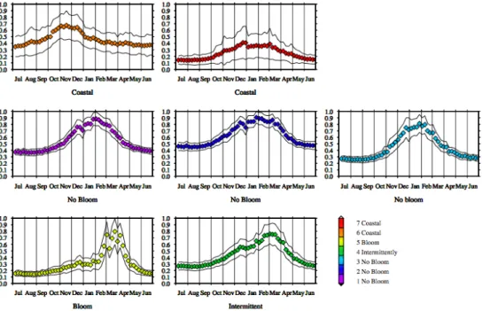
In general, the structure and the spatial classification of the Mediterranean pixels, as obtained with the K-means proce-dure, are very consistent (Fig. 4). The geographical bound-aries between the clusters are reasonably well defined and the within-cluster heterogeneity is very low. The associated tem-poral evolutions of the 7 centers are plotted with the relative +/− one standard deviation (Fig. 5). It is worth remember-ing that the only constraints imposed to the K-means analysis were: 1) the number of the clusters and 2) the normalization performed on the climatological time series. The first was chosen on the basis of a test indicating the maximum number of clusters statistically significant/important for the SeaWiFS data set.
To better discuss the results, clusters were grouped again in four bigger classes, using, as a discriminating criterion, the position of the yearly maximum in the temporal evolution of the cluster’s centers.
5˚W 0˚ 5˚E 10˚E 15˚E 20˚E 25˚E 30˚E 35˚E 30˚N
35˚N 40˚N 45˚N
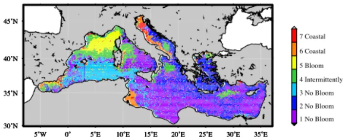
5˚W 0˚ 5˚E 10˚E 15˚E 20˚E 25˚E 30˚E 35˚E 30˚N 35˚N 40˚N 45˚N 1 No Bloom 2 No Bloom 3 No Bloom 4 Intermittently 5 Bloom 6 Coastal 7 Coastal
5˚W 0˚ 5˚E 10˚E 15˚E 20˚E 25˚E 30˚E 35˚E 30˚N
35˚N 40˚N 45˚N
2008 Jan 8 18:38:02 D’Ortenzio & Ribera, Fig. 4
Fig. 4. Spatial distribution of the clusters obtained from the k-means analysis.
In more detail: The north western area of the basin is classed as a unique, unambiguous, cluster (#5). Its time course displays a peak in late winter-early spring months. In the other months, the values are close to the background line (generally less than 25% of the maximum values), differing slightly between winter and summer/fall.
Another cluster (#4) encompasses several regions dissemi-nated all over the basin (the South Adriatic gyre, the area off-shore of the North-Western Ionian Italian, the Rhodes Gyres, the Western Tyrrhenian, the Balearic front, the Liguro-Provencal current and, partially, the Alboran sea). The tem-poral evolution of this class shows its maximum in February-March, with an appreciable increase in October and a less pronounced difference between minima and maxima than in cluster #5.
Two clusters (#6 and #7) are limited to the Northern and Western Adriatic boundaries, and to a few spots in coastal areas. The first cluster (#6) displays a pronounced maximum (up to a two fold increase of the background biomass value) in late summer-early autumn. For the second cluster (#7) the seasonal signal is barely evident, with very similar values all the year round (range=0.1–0.3).
The three residual clusters (#1, #2, #3) cover the rest of the basin (about 60% of the total area), following a well-defined, though not an exclusively geographical distribution: one is prevalently located in the Algerian Basin (#3), another (#1)
southward of the 35◦ parallel and in the Tyrrhenian Basin,
and the last (#2) almost entirely covers the Aegean, the Adri-atic and the Central Ionian basins. The temporal trends of these clusters are similar, showing a bimodal dynamic, with higher and quite constant values in fall-winter and lower and uniform values in late spring-summer. The slight differences observed concern the time of the decrease, which is Febru-ary for cluster #3 and March for cluster #2 and #1. The rise is in mid-September for all of them. Furthermore, the con-centration span between minima and maxima increases from cluster #2 (factor less than 2) to cluster #1 (around 2) to clus-ter #3 (more than 2).
The last three clusters have a more patchy distribution that is particularly evident along the boundaries they have in com-mon (e.g., the South Western Ionian) with a lot of
interweav-ing. This is definitely not the case for the other clusters, which are geographically well localized. Moreover, most of the cluster’s time series exhibit small dispersion around the mean values (continuous lines in Fig. 5, evaluated by a +/− one standard deviation), which indicates that the classifica-tion is able to group essentially similar time series together. Cluster #7 constitutes an exception, as the spreading of the data encompass most of the dynamic range.
To test the relevance and the stability of the regionaliza-tion, a series of statistical tests were performed. The orig-inal data set has been modified, introducing different de-grees of noise (see later) and then creating several “test” data sets. The clusterization was then applied to each modified data sets and the results were then compared to the clus-ters obtained from the original data set. The comparison was performed using as metric parameter the Jaccard coefficient (Henning, 2007 and references therein), which indicates the proportion of points belonging to both sets to all the points involved in at least one of the sets. A value of 0.7, or greater, indicates that the cluster is stable (Henning, 2007). Three different types of modified data sets were produced: a “boot strap”, which uses the obtained clusters to introduce bias in the data sets, a “noise”, which randomly replaces a percent-age of points (5% in our case) in the original data set with noise points, and “jittering”, which adds noise or error to ev-ery single point in the original data set. Noise and errors for the “noise” and “jittering” data sets were calculated using the procedure indicated by Henning (2007), which is based on the covariance matrix of the original data set. For each type of test, 15 data sets were produced and for each data set, the Jaccard parameter was calculated. Finally, the average of the Jaccard parameter is retained. The results are summa-rized in Table 1. Only cluster 6 shows a Jaccard parameter below 0.7 for the “boot strap” and the “noise” tests, while all the other clusters have high values of the Jaccard coefficient. The three tests demonstrated that the applied clusterization is sufficiently stable and that the obtained clusters, with the noticeable exception of the #6, remain practically unaltered when the original data set is modified.
To summarize, a well resolved zonation of the Mediter-ranean basin was obtained applying the k-means clusters analysis to the normalized climatological SeaWiFS data.
The link between the three classes introduced above (“blooming”, “non-blooming” and “intermittently blooming” zones) and the new classification can be evaluated by com-paring panels in Fig. 5.
Cluster #5 definitely corresponds to the “blooming” areas, while the big class including clusters #1, #2 and #3 matches the previous definition of the “non-blooming” regions. Clus-ter #4 identifies regions with erratic regimes, which combine periods of intense biomass accumulation with oligotrophic conditions, and then it can likely be associated to our def-inition of the “intermittently blooming” zones. Finally, the big class encompassing clusters #6 and #7 defines another regime, mainly related to the coastal areas. The “coastal”
F. D’Ortenzio and M. Ribera d’Alcal`a: On the trophic regimes of the Mediterranean Sea 145
Fig. 5. Temporal evolution of the centers of the clusters obtained from the k-means analysis. The colors of the curves follow the same color scale of Fig. 4. Lower panels: “Bloom” and “Intermittently blooming” areas (clusters #4 and #5). Middle panels: “No-bloom” regions (clusters #1, #2, #3). Upper panels: “Coastal” regions (clusters #6 and #7). Continuous lines indicate the relative +/− one standard deviation (see text).
Table 1. Results of the cluster’s stability tests.
Cluster 1 Cluster 2 Cluster 3 Cluster 4 Cluster 5 Cluster 6 Cluster 7
Boot strap 0.830 0.821 0.851 0.789 0.884 0.611 0.916
Noise 0.815 0.803 0.876 0.776 0.911 0.676 0.955
Jittering 0.889 0.883 0.914 0.870 0.913 0.826 0.940
regimes, which were barely visible in the Hovm¨oller diagram of transect 2, but are more evident in the climatological map of the whole basin (Fig. 1).
4 Discussion and conclusions
The proposed classification, while more statistically robust, does not substantially deviate from what already proposed by previous studies (Morel and Andre’, 1991; Antoine et al., 1995; Bosc et al., 2004). The comparison between the clima-tological mean (figure 1) and the clusters distribution (Fig. 5) confirms this point. Therefore, we infer that it is the struc-ture of the seasonal cycle that determines intense or moderate accumulation of phytoplankton biomass.
This point is not trivial and it represents an unexpected result. The geographical distribution of the clusters, deter-mined by the seasonal cycle of phytoplankton biomass, is tightly coupled with the dynamic range of biomass itself, as obtained, for example, from the mean of 10 years of
clima-tological data (i.e. Fig. 1). Oligotrophic regions, showing very low mean values of chlorophyll concentration, match exactly with clusters #1, 2, 3, whereas, productive regions have relevantly different seasonal cycles (cluster #4, 5). In other words, at least in the Mediterranean, accumulations of phytoplankton are observed only where a specific temporal trend is present.
Furthermore, the different Mediterranean seasonal cycles correspond to different “trophic regimes” sensu Longhurst. In fact, the chlorophyll time course of the Longhurst model number 3 follows a very similar trend to the “non-blooming” classification of the present study (clusters #1–3), which
actually represents 60% of the Mediterranean basin. On
the other hand, our “blooming” regime (cluster #5) appears very similar to model number 2 of the Longhurst classifica-tion, demonstrating that, at least in some areas, the Mediter-ranean follows North-Atlantic-like dynamics. The Longhurst coastal biome is also represented (our clusters #6 and #7), but with some important differences. In his reconstruction,
upwelling and tides play a major role. Almost all the areas in our coastal clusters are not proper coastal upwelling ar-eas and none of them depend directly on tidal mixing. Pixels from cluster #7 have a spotty distribution with the exception of Northern Adriatic, the Gulf of Lion area and the North Aegean region.
Our cluster #6 displays its maximal values during the late summer-fall period and a further decrease in winter. We ad-vance the following hypothesis: the fall increase may reflect the response to the disruption of pycnocline, which, in a shal-low area, could be particularly effective through the recircu-lation of the bottom reservoir (both of nutrients and biota). The later decrease of biomass is likely due to flushing by lat-eral water masses, which carry a lower amount of autotrophic biomass.
The most interesting group is cluster #4, which we classi-fied as “intermittently blooming”. Intermittence is certainly a manifestation of the interannual variability as also discussed by Longhurst, but it is crucial to understand which changes in the mechanisms are responsible for it. Some areas belong-ing to cluster #4 are areas of cyclonic circulation (Rhodes, South Adriatic, Northern Tyrrhenian) while the other areas are not. Their seasonal cycle displays a progressive increase in biomass from September to February. We speculate that this cycle is an overlap of the typical autumnal bloom of temperate regions followed by a progressive deepening of the thermocline and/or the subsequent vertical transport due to cyclonic or mesoscale frontal dynamics. Interestingly, we found that none of Longhurst’s oceanic provinces would match the pattern of cluster #4. We believe that, if our hy-pothesis about the role of flushing is correct, the explanation is that Longhurst analysis focused on much larger scales.
As Mediterranean is considered an oligotrophic ocean, we now focus our discussion on the oligotrophic clusters, i.e. the clusters that encompass the areas showing the lower values of chlorophyll concentration (#1, 2, 3). The “non-blooming” clusters (#1, 2, 3) display a similar seasonal cycle, with low biomass during late spring-summer and higher biomass up to the maxima in late fall-winter. The differences between them are in the ranges between maximum and minimum: cluster #3 displays the highest range (approximately 3:1 ratio) and cluster #2 the lowest (approximately 2:1). Differences are also noticeable in the inflections of the curve, with cluster 1 and 2 displaying a smooth rise and cluster #3 a steeper rise around October and a steeper decrease around mid-January. Looking at the distribution of the pixels for each cluster (Fig. 4) and at the mixed layer climatology by D’Ortenzio et al. (2005) our interpretation of the “non-blooming” clus-ters is the following. Cluster #3 is driven by the Atlantic wa-ter inflow. Assuming a transit time of two to four months from Gibraltar to the area (Millot, 1999), the surface wa-ter in September-November should be severely deprived of nutrients and biomass, entering the basin as a summer At-lantic surface water. The steep biomass increase from Oc-tober to December is supported by the progressive, though
moderate, deepening of the mixed layer within the area (e.g., D’Ortenzio et al., 2005 their Fig. 1). We also hypothesize that the phytoplankton biomass is only moderately controlled by grazing. In January and February there is a further deep-ening of the mixed layer, which produces a slight dispersal of biomass in the water column, with possibly a higher depth in-tegrated biomass. At the time of re-stratification (e.g. March) there are no more new nutrients to be used, which precludes any shift-up of phytoplankton biomass. We advance the hy-pothesis that the decrease is not only the result of the biolog-ical pump but derives also from the effect the redistribution of carbon within the food web with an increased ratio of con-sumers vs. primary producers. The time course of the other two “non blooming” clusters is quite similar to cluster #3 and displays a quasi-bimodal pattern: higher biomass from mid-October to mid-March and lower biomass in the remaining period. It is worth noting that the high biomass interval over-laps with the period when irradiance is at its minimum.
Our analysis demonstrated that the possible latitudinal gra-dient in the Mediterranean biomass is perturbed by regional processes that prevent the formation of a single trend. The Mediterranean seasonal signal is smoothed according to pat-terns typical of sub-tropical regions, which have different characteristics in the different Mediterranean areas. Most of the basin is characterized by early biomass enhancements, which last for 2–3 months depending on the region. They are not intense (although chlorophyll concentration doubles) as only very late blooms can exploit enough new nutrients to allow significant build-ups of biomass, which can be ini-tially uncoupled by consumers. This is the case of the clas-sical spring bloom regime, which also occurs in the basin: regularly (in the North Western Mediterranean) and intermit-tently (in four specific areas). We also speculate that each regime hosts a slightly different food web and that any shifts in the regime will result primarily in a rearrangement of the clusters, thus making the ocean color a tool for prompt de-tection of climate impact in the basin. Therefore, the view of the Mediterranean Sea as a good macrocosm to monitor changes in food web structure in relation to changes in ex-ternal forcing is somehow supported by the reduced space scales in which ecoclines take place.
Finally, it is interesting to compare the Mediterranean
provinces with the oceanic ones. It is well known that
the North Atlantic hosts the most intense (in terms of both temporal and spatial extension) phytoplankton bloom of the global ocean (see Duklow and Harris, 1993). The timing of the North Atlantic blooms onset and development are not uniform along the whole North Atlantic region. Following the analysis reported by Siegel et al. (2002), the blooms in
the regions located between 35◦N and 45◦N start in the first
days of the year (January–February), whereas in the north-ern region (where the highest concentrations are observed) the bloom onset occurs later in spring (March–April). The “bloom period” is identified in January–February, in
F. D’Ortenzio and M. Ribera d’Alcal`a: On the trophic regimes of the Mediterranean Sea 147
and 45◦–55◦N respectively. In the Mediterranean, the same
“mixture” of trophic regimes is embedded in a narrower
lat-itudinal range (30◦–43◦N). Therefore, even if the
tempo-ral dynamics are similar, the Mediterranean system appears shifted in time (or in latitude, depending on the perspective) compared to the corresponding regions in the North Atlantic following the same Longhurst model.
The meridional limit of the NA bloom is generally
lo-cated between 35◦and 40◦North, with biomass
concentra-tions increasing with latitude. South of this limit, the trophic regime is considered tropical or sub-tropical, thus charac-terized by a strong oligotrophy and a weak seasonal vari-ability. The Mediterranean is located on the boundary of these two regions, with the “non-blooming” areas exhibiting a sub-tropical regime, interleaved with areas (i.e. the “bloom-ing” an the “intermittently bloom“bloom-ing” regions) where, under particular conditions (both atmospheric and hydrographic), North Atlantic bloom-like events take place.
Acknowledgements. The US NASA space agency is thanked for
the easy access to SeaWiFS data. The authors are also grateful to Herv´e Claustre and Louis Prieur, for their helpful comments and suggestions. The authors would also like to acknowledge Salvatore Marullo and Rosalia Santoleri. Without their pioneering works on remote sensing analysis in the Mediterranean and their sharing of knowledge of remote sensing techniques, this work would have never been possible.
Edited by: E. Boss
References
Antoine, D., D’Ortenzio, F., Hooker, S. B., Becu, G., Gentii, B., Taillez, D., and Scott, A. J.: Assessment of uncertainty in the ocean reflectance determined by three satellite ocean color sen-sors (MERIS, SeaWiFS and MODIS-A) at an offshore site in the Mediterranean Sea (BOUSSOLE project), J. Geophys. Res. (C. Oceans), 113, C07013, doi:10.1029/2007JC004472, 2008. Antoine, D., Morel, A., and Andr´e, J. M.: Algal pigment
distri-bution and primary production in the eastern Mediterranean as derived from CZCS observations, J. Geophys. Res., 100, 16193– 16210, 1995.
Ball, G. H. and Hall, D. J.: A clustering technique for summarizing multivariate data, Behavioral Science, 12, 153–155, 1965. Bosc, E., Bricaud, A., and Antoine, D.: Seasonal and
interan-nual variability in algal biomass and primary production in the Mediterranean Sea, as derived from four years of Sea-WiFS observations, Glob. Biogeochem. Cy., 18, GB1005, doi:10.1029/2003GB002034, 2004.
Calinski, T. and Harabasz, J.: A dendrite method for cluster analy-sis, Communications in statistics, 3, 1–27, 1974.
Claustre, H., Morel, A., Hooker, S. B., Babin, M., Antoine, D., Oubelkheir, K., Bricaud, A., Leblanc, K., Qu´eguiner, B., and Maritorena, S.: Is desert dust making oligotrophic waters greener?, Geophys. Res. Lett., 29, 107–111, 2002.
D’Ortenzio, F., Iudicone, D., Montegut, C. D., Testor, P., Antoine, D., Marullo, S., Santoleri, R., and Madec, G.: Seasonal vari-ability of the mixed layer depth in the Mediterranean Sea as
derived from in situ profiles, Geophys. Res. Lett., 32, L12605, doi:10.1029/2005GL022463, 2005.
D’Ortenzio, F., Marullo, S., Ragni, M., d’Alcal`a, M. R., and San-toleri, R.: Validation of empirical SeaWiFS chlorophyll-a algo-rithms retrieval in the Mediterranean Sea: a case study for olig-otrophic seas, Remote Sens. Environ., 82, 79–94, 2002. D’Ortenzio, F., Ragni, M., Marullo, S., and d’Alcala, M. R.:
Did biological activity in the Ionian Sea change after the
East-ern Mediterranean Transient? Results from the analysis of
remote sensing observations, J. Geophys. Res., 108, 8113, doi:10.1029/2002JC001556, 2003.
Devred, E., Platt, T., and Sathyendranath, S.: Delineation of eco-logical provinces using ocean colour radiometry, Mar. Ecol. Progress S., 346, 1–7, 2007.
Ducklow, H. and Harris, R.: Introduction to the JGOFS North At-lantic Bloom Experiment, Deep Sea Res. II, 40, 1–4, 1993. Gacic, M., Civitarese, G., Miserocchi, S., Cardin, V., Crise, A., and
Mauri, E.: The open-ocean convection in the Southern Adriatic: a controlling mechanism of the spring phytoplankton bloom, Continental Shelf Research, 22, 1897–1908, 2002.
Hartigan, J. H.: Clustering Algorithms, Wiley, New York, 351 pp., 1975.
Hartigan, J. H. and Wong, M. A.: A K-Means clustering algorithm., Appl. Stat., 28, 100–108, 1979.
Henning, C.: Cluster-wise assessment of cluster stability Computa-tional Statistics and Data Analysis, 52, 258–271, 2007. Longhurst, A. R.: Ecological Geography of the Sea, edited by:
Press, A., Elsevier Science, New York, 552 pp., 1998.
Marty, J. C., Chiaverini, J., Pizay, M. D., and Avril, B.: Seasonal and interannual dynamics of nutrients and phytoplankton pig-ments in the western Mediterranean Sea at the DYFAMED time-series station (1991–1999), Deep Sea Res. II, 49, 1965–1985, 2002.
McClain, C. R., Feldman, G. C., and Hooker, S. B.: An overview of the SeaWiFS project and strategies for producing a climate research quality global ocean bio-optical time series, Deep Sea Res. Part II, 51, 5–42, 2004.
Milligan, G. W. and Cooper, M. C.: An examination of procedures for determining the number of clusters in a data set, Psychome-trika, 50, 159–179, 1985.
Millot, C.: Circulation in the Western Mediterranean sea, J. Mar. Syst., 20, 423–442, 1999.
Morel, A. and Andr´e, J. M.: Pigment distribution and primary pro-duction in the western Mediterranean as derived from CZCS ob-servations, J. Geophys. Res., 96, 12685-12691, 1991.
Morel, A. and Berthon, J. F.: Surface pigments, algal biomass pro-files, and potential production of the euphotic layer: relationship reinvestigated in view of remote-sensing applications, Limnol. Oceanogr., 34, 1545–1562, 1989.
O’Reilly, J. E., Maritorena, S., Mitchell, B. G., Siegel, D. A., Carder, K. L., Garver, S. A., Kahru, M., and McClain, C.: Ocean color chlorophyll algorithms for SeaWiFS, J. Geophys. Res., 103, 937–924, 1998.
Oguz, T., Tugrul, S., Kideys, A. E., Ediger, V., and N., K.: Physical and biogeochemical characteristics of the Black Sea in: The Sea, edited by: Robinson, A. R. and Brink, K. H., Harvard University Press, Cambridge (MA), 1331–1369, 2004.
Pinardi, N. and Masetti, E.: Variability of the large scale general circulation of the Mediterranean Sea from observations and
eling: a review, Palaeogeography Palaeoclimatology Palaeoecol-ogy, 158, 153–174, 2000.
Ratkowsky, D. A. and Lance, G. N.: A criterion for determining the number of groups in a classification, Australian Computer Journal, 10, 115–117, 1978.
Santoleri, R., Banzon, V., Marullo, S., Napolitano, E., D’Ortenzio, F., and Evans, R.: Year-to-year variability of the phytoplankton bloom in the southern Adriatic Sea (1998–2000): Sea-viewing Wide Field-of-view Sensor observations and modeling study, J. Geophys. Res., 108, 8122, doi:10.1029/2002JC001636, 2003. Sathyendranath, S. and Platt, T.: Remote sensing of oceanic
chloro-phyll: consequence of nonuniform pigment profile, Appl. opt., 28, 490–495, 1989.
Siegel, D. A., Doney, S. C., and Yoder, J. A.: The North Atlantic spring phytoplankton bloom and Sverdrup’s critical depth hy-pothesis, Science, 296, 730–733, 2002.
Sournia, A.: La production primaire planctonique en Mediterranee: Essai de mise a jour, Bull. Et. Comm. Medit. Special Issue 5, 1–128, 1973.
Volpe, G., Santoleri, R., Vellucci, V., Ribera d’Alcala, M., Marullo, S., and D’Ortenzio, F.: The colour of the Mediterranean Sea: global versus regional bio-optical algorithms evaluation and im-plication for satellite chlorophyll estimates, Remote Sens. Envi-ron., 107, 625–638, 2007.