Apparent optical properties of the Canadian Beaufort Sea – Part 1: Observational overview and water column relationships

HAL Id: hal-01532188

https://hal.sorbonne-universite.fr/hal-01532188

Submitted on 2 Jun 2017

HAL is a multi-disciplinary open access

archive for the deposit and dissemination of

sci-entific research documents, whether they are

pub-lished or not. The documents may come from

teaching and research institutions in France or

abroad, or from public or private research centers.

L’archive ouverte pluridisciplinaire HAL, est

destinée au dépôt et à la diffusion de documents

scientifiques de niveau recherche, publiés ou non,

émanant des établissements d’enseignement et de

recherche français ou étrangers, des laboratoires

publics ou privés.

Sea – Part 1: Observational overview and water column

relationships

David Antoine, S.B. Hooker, S Bélanger, A Matsuoka, M Babin

To cite this version:

David Antoine, S.B. Hooker, S Bélanger, A Matsuoka, M Babin. Apparent optical properties of

the Canadian Beaufort Sea – Part 1: Observational overview and water column relationships.

Bio-geosciences, European Geosciences Union, 2013, 10 (7), pp.4493-4509. �10.5194/bg-10-4493-2013�.

�hal-01532188�

Biogeosciences, 10, 4493–4509, 2013 www.biogeosciences.net/10/4493/2013/ doi:10.5194/bg-10-4493-2013

© Author(s) 2013. CC Attribution 3.0 License.

EGU Journal Logos (RGB)

Advances in

Geosciences

Open Access

Natural Hazards

and Earth System

Sciences

Annales

Geophysicae

Nonlinear Processes

in Geophysics

Atmospheric

Chemistry

and Physics

Atmospheric

Chemistry

and Physics

Atmospheric

Measurement

Techniques

Atmospheric

Measurement

Techniques

Biogeosciences

Open Access Open Access

Biogeosciences

Discussions

Climate

of the Past

Open Access Open Access

Climate

of the Past

Discussions

Earth System

Dynamics

Open Access Open Access

Earth System

Dynamics

Geoscientific

Instrumentation

Methods and

Data Systems

Open Access

_{Geoscientific}

Instrumentation

Methods and

Data Systems

Geoscientific

Model Development

Open Access Open Access

Geoscientific

Model Development

Hydrology and

Earth System

Sciences

Hydrology and

Earth System

Sciences

Ocean Science

Open Access Open Access

Ocean Science

Solid Earth

Open Access Open Access

Solid Earth

The Cryosphere

Open Access Open Access

The Cryosphere

Discussions

Natural Hazards

and Earth System

Sciences

Open Access

Discussions

Apparent optical properties of the Canadian Beaufort Sea – Part 1:

Observational overview and water column relationships

D. Antoine1,*, S. B. Hooker2, S. B´elanger3, A. Matsuoka4, and M. Babin1,4

1_{Laboratoire d’Oc´eanographie de Villefranche (LOV), UMR7093, Centre National de la Recherche Scientifique (CNRS) and}

Universit´e Pierre et Marie Curie, Paris 06, Villefranche-sur-Mer, France

2_{NASA Goddard Space Flight Center, Ocean Ecology Laboratory, Greenbelt, Maryland 20771, USA}

3_{Universit´e du Qu´ebec `a Rimouski, D´epartement de biologie, chimie et g´eographie and BOR ´EAS, Rimouski (Qu´ebec),}

Canada

4_{Unit´e Mixte Internationale Takuvik, Centre National de la Recherche Scientifique (CNRS) and Universit´e Laval, Avenue de}

la M´edecine, Qu´ebec City (Qu´ebec), Canada

*_{now at: Curtin University, Department of Imaging and Applied Physics, Remote Sensing and Satellite Research Group,}

Perth, WA 6845, Australia

Correspondence to: D. Antoine (antoine@obs-vlfr.fr)

Received: 2 February 2013 – Published in Biogeosciences Discuss.: 1 March 2013 Revised: 30 May 2013 – Accepted: 5 June 2013 – Published: 4 July 2013

Abstract. A data set of radiometric measurements collected

in the Beaufort Sea (Canadian Arctic) in August 2009 (Ma-lina project) is analyzed in order to describe apparent op-tical properties (AOPs) in this sea, which has been subject to dramatic environmental changes for several decades. The two properties derived from the measurements are the spec-tral diffuse attenuation coefficient for downward irradiance,

Kd, and the spectral remote sensing reflectance, Rrs. The

for-mer controls light propagation in the upper water column. The latter determines how light is backscattered out of the water and becomes eventually observable from a satellite ocean color sensor. The data set includes offshore clear wa-ters of the Beaufort Basin as well as highly turbid wawa-ters of the Mackenzie River plumes. In the clear waters, we show

Kd values that are much larger in the ultraviolet and blue

parts of the spectrum than what could be anticipated consid-ering the chlorophyll concentration. A larger contribution of absorption by colored dissolved organic matter (CDOM) is responsible for these high Kd values, as compared to other

oligotrophic areas. In turbid waters, attenuation reaches ex-tremely high values, driven by high loads of particulate mate-rials and also by a large CDOM content. In these two extreme types of waters, current satellite chlorophyll algorithms fail. This questions the role of ocean color remote sensing in the Arctic when Rrsfrom only the blue and green bands are used.

Therefore, other parts of the spectrum (e.g., the red) should be explored if one aims at quantifying interannual changes in chlorophyll in the Arctic from space. The very peculiar AOPs in the Beaufort Sea also advocate for developing spe-cific light propagation models when attempting to predict light availability for photosynthesis at depth.

1 Introduction

Current dramatic evolutions of the Arctic environment in-clude an increase in atmosphere temperature larger than else-where (Zhang, 2005), a summer ice melting that acceler-ates as compared to current model predictions (Stroeve et al., 2005), carbon-rich permafrost thawing on most coastal fringes (Schuur et al., 2008), and cloudiness changes (East-man and Warren, 2010). These major changes in physical and chemical forcing inevitably lead to significant modifi-cations of the underwater light environment of Arctic wa-ters, through their impact on seawater optical properties. A cascade of effects is to be expected on all light-mediated or light-controlled processes, including photosynthesis and photochemical reactions, and the heating rate of the upper layers.

Quantifying the impact of current changes in optical prop-erties requires knowledge of them prior to these changes. Es-tablishing such a baseline is actually difficult because op-tical properties of Arctic waters have been scarcely sam-pled until now. Reports have been made of inherent opti-cal properties (IOPs, sensu Preisendorfer, 1961), for instance in surface waters of the Chukchi Plateau (Pegau, 2002) or in the Beaufort and Chukchi seas in August 2000 (Wang et al., 2005). The Malina Leg2b cruise has brought addi-tional IOP observations, in particular of particulate absorp-tion (B´elanger et al., 2013), absorpabsorp-tion by colored dissolved organic matter (CDOM; Matsuoka et al., 2013), and partic-ulate backscattering (Doxaran et al., 2012). Other data were essentially collected in relation to quantifying upper ocean heating rates close to or below sea ice (Pegau, 2002, and ref-erences therein). Observations of apparent optical properties (AOPs) in the Arctic are even more rare. Smith (1973) re-ported irradiance measurements made below a 5 m thick ice-cap in the central Arctic (on Fletcher’s ice island T-3), and Maykut and Grenfell (1975) reported irradiance measure-ments also made under sea ice (∼ 1–2 m thick) near Point Barrow, Alaska. Smith (1973) concluded that Arctic waters were among the clearest in the world known at that time. The rationale in the 1970s and 1980s was definitely to understand under-ice conditions, which were prevailing and considered as the typical Arctic environment, whereas a different per-spective now emerges because large areas are free of ice in summer.

In the 1980s, Topliss et al. (1989) performed spectral Kd

measurements in the northern Baffin Bay, eastern Canadian Arctic, suggesting that the waters from this region departed significantly from the so-called case-1 waters (Morel and Prieur, 1977) because of the presence of an anomalously high particulate scattering background, as well as a greater contri-bution of the degradation products to blue light attenuation. Accordingly, Mitchell (1992) noticed an important contribu-tion of yellow substances to the blue light attenuacontribu-tion in Fram Strait and in the Barents Sea relative to the polar Antarctic waters. He showed that polar phytoplankton tend to present higher pigment-packaging effect relative to temperate lati-tudes that reduces their efficiency to absorb light for a given concentration of chlorophyll a (Chl a).

Historical observations were complemented only much more recently by measurements made in ice-free waters (Wang and Cota, 2003; Matsuoka et al., 2007, 2009, 2011; Hill, 2008; Ben Mustapha et al., 2012; Brunelle et al., 2012), and no other measurements have been reported in between in the open literature, at least to our knowledge. Therefore, at-tenuation and reflectance properties of Arctic waters are still poorly known.

Here we report on an intense program of radiometric data collection that was carried out during the Malina Leg2b cruise in the Canadian Beaufort Sea in August of 2009. The large number of sampled stations makes this effort appropri-ate to characterize the underwappropri-ater light field in this region.

The objective is to describe the data set in terms of the spec-tral diffuse attenuation coefficient for downward irradiance,

Kd(λ), and the spectral remote sensing reflectance, Rrs(λ).

The former controls light propagation in the upper water col-umn and therefore modulates the heating rate and the light availability for photosynthesis or photochemical reactions. The latter is a measure of the light backscattered out of the water and eventually observable from a satellite ocean color sensor.

The different light environments that were encountered are first described, and a classification is proposed for the sta-tions that were sampled in a variety of environments. Spectral characteristics and membership to either case-1 or case-2 wa-ters is discussed, and the results from a search for bio-optical relationships are presented. The implications of our findings on the modeling of primary production and the remote sens-ing of Chl a in the Arctic are finally discussed.

A second objective of this paper and especially of its com-panion part II paper (Hooker et al., 2013) is to illustrate the capabilities of a next-generation profiler system that we used for collection of the radiometric data. This instrument provides high-quality radiometric measurements over an ex-tended spectral range as compared to previously used pro-filing systems, which is particularly adapted to the multi-faceted Arctic environment.

2 Methods

2.1 Deriving AOPs from in-water profiles of radiometric quantities

Vertical profiles of radiometric quantities were collected dur-ing Malina Leg2b usdur-ing a biospherical Compact-Optical Pro-filing System (C-OPS). The rationale for the development of this next-generation in-water profiling system is provided in the companion paper (Hooker et al., 2013), along with de-tailed description of its design and operation, and further demonstration of its capability in deriving high-accuracy ra-diometric data in particular just below the surface. Suffice it to say here that this instrument allows getting high-resolution vertical profiles of the downward plane irradiance, Ed, and

the upwelling radiance at nadir, Lu, in the following 19

spec-tral bands: 320, 340, 380, 395, 412, 443, 465, 490, 510, 532, 555, 560, 625, 665, 670, 683, 710, 780 nm and photosynthet-ically active radiation (PAR). The high dynamic range of the microradiometers used in the C-OPS in principle allows get-ting Edand Luover 8 orders of magnitude, from high

irradi-ances typical of the surface layer during a sunny day in clear waters to dim irradiances under cloudy skies or at large depth or in extremely turbid waters. The C-OPS was deployed from a 12 m barge in parallel to, but at distance from, the

Amund-sen icebreaker main operations. This protocol allowed

avoid-ing any ship perturbation, either due to shadowavoid-ing from the hull and superstructures or due to mixing of the upper layers.

It also allowed an easy and unobstructed deployment of the deck reference using a telescoping mast (Hooker, 2010) for collection of above-surface downward irradiance (Ed(0+)or

Es; see below), and getting close to icecaps for specific casts.

The processing of these data is based here on a well-established methodology (Smith and Baker, 1984) that was evaluated in an international round robin (Hooker et al., 2001) and shown to be capable of agreement at the 1 % level when the processing options were as similar as possible. Complete details of the terms and dependencies are avail-able in the Ocean Optics Protocols (hereafter, the Protocols), which initially adhered to the Joint Global Ocean Flux Study (JGOFS) sampling procedures (JGOFS, 1991) and defined the standards for NASA calibration and validation activities (Mueller and Austin, 1992). Over time, the Protocols were initially revised (Mueller and Austin, 1995) and then updated annually (Mueller 2000, 2002, 2003).

The Protocols are detailed, so only a brief overview for ob-taining data products from vertical profiles of upwelling radi-ance (Lu)plus upward and downward irradiance (Euand Ed,

respectively) is presented here. In-water radiometric quanti-ties in physical units, ℵ (i.e., Lu, Eu, or Ed), are normalized

with respect to simultaneous measurements of the global so-lar irradiance, Ed(0+, λ, t), with t explicitly expressing the

time dependence, according to

ℵ(z, λ, t0) = ℵ(z, λ, t )

Ed(0+, λ, t0)

Ed(0+, λ, t )

, (1)

where ℵ (z, λ, t0) identifies the radiometric parameters as

they would have been recorded at all depths z at the same time t0, and t0is generally chosen to coincide with the start

of data acquisition. For simplicity, the variable t is omitted in the following text. In addition, any data collected when the vertical tilt of the profiler exceeds 5◦are excluded from the ensuing analysis.

After normalization and tilt filtering, a near-surface por-tion of Ed (z, λ) centered at z0 and having homogeneous

optical properties (verified with temperature and attenuation parameters) extending from z1=z0+1zand z2=z0−1z

is established separately for the blue-green and red wave-lengths; the ultraviolet (UV) is included in the interval most similar to the UV attenuation scales. Both intervals begin at the same shallowest depth, but the blue-green interval is al-lowed to extend deeper if the linearity in [Lu(z, λ)], as

deter-mined statistically, is thereby improved. The negative value of the slope of the regression yields the diffuse attenuation coefficient, Kd(λ), which is used to extrapolate the fitted

por-tion of the Edprofile through the near-surface layer to null

depth, z = 0−.

Fluctuations caused by surface waves and so-called lens

effects prevent accurate measurements of Ed(λ)close to the

surface (Zaneveld et al., 2001). A value just below the surface (at null depth z = 0−)can be compared to that measured con-temporaneously above the surface (at z = 0+)with a separate

solar reference using

Ed(0−, λ) =0.97Ed(0+, λ), (2)

where the constant 0.97 represents the applicable air–sea transmittance, Fresnel reflectances, and the irradiance re-flectance (Eu/Ed), and is determined to an accuracy better

than 1 % for solar elevations above 30◦_{and low-to-moderate}

wind speeds. The distribution of Ed measurements at any

depth z influenced by wave-focusing effects does not fol-low a Gaussian distribution, so linear fitting of Edin a

near-surface layer is poorly constrained, especially if the number of samples is small. The application of (2) to the fitting pro-cess establishes a boundary condition or constraint for the fit (Hooker and Brown, 2013).

The appropriateness of the Edextrapolation interval,

ini-tially established by z1 and z2, is evaluated by determining

if (2) is satisfied to within approximately the uncertainty of the calibrations (a few percent); if not, z1and z2are

redeter-mined – while keeping the selected depths within the shal-lowest homogeneous layer possible – until the disagreement is minimized (usually to within 5 %). The linear decay of ln[ℵ (z, λ)] for all light parameters in the chosen near-surface layer is then evaluated, and if linearity is acceptable, the en-tire process is repeated on a cast-by-cast basis. Subsurface primary quantities at null depth, ℵ (0−, λ), are obtained from the slope and intercept given by the least-squares linear re-gression of ln[ℵ (z, λ)] versus z within the extrapolation in-terval specified by z1and z2.

The processing uses two extrapolation intervals, one for the UV-green and one for the red-NIR. Both intervals start at the same depth, but the UV-green is allowed to extend deeper, because the attenuation is frequently less, as long as that part of the water column that is involved remains homogeneous. The average extrapolation intervals are in the top 1.5–3 m of the water column for the UV-green, and in the top 1–2 m for the red and near infrared.

The water-leaving radiance is obtained directly from

Lw(λ) =0.54Lu(0−, λ), (3)

where the constant 0.54 accurately accounts for the partial reflection and transmission of the upwelled radiance through the sea surface, as confirmed by Mobley (1999). To account for the aforementioned dependence of Lw on the solar flux,

which is a function of atmospheric conditions and time of day, Lw is normalized by the (average) global solar

irradi-ance measured during the time interval corresponding to z1

and z2:

Rrs(λ) =

Lw(λ)

Ed(0+, λ)

(4)

where Rrsis the remote sensing reflectance. Normalized

vari-ables are the primary input parameters for inverting TChl a concentration from in situ optical measurements as part of

the “OC” class of algorithms (O’Reilly et al., 1998), which means they are central variables for validation exercises.

An additional refinement includes the bidirectional nature of the upwelled radiance field, which is to a first approx-imation dependent on the solar zenith angle. An early at-tempt to account for the bidirectionality of Lw by Gordon

and Clark (1981), following Austin (1974), defined a nor-malized water-leaving radiance, [Lw(λ)]N, as the

hypotheti-cal water-leaving radiance that would be measured in the ab-sence of any atmospheric loss with a zenith Sun at the mean Earth–Sun distance. The latter is accomplished by adjusting

Rrs(λ)with the time-dependent mean extraterrestrial solar

ir-radiance, F0 (ignoring all dependencies except wavelength

for brevity):

[Lw(λ)]N=F0(λ)Rrs(λ), (5)

where F0(λ)is usually formulated to depend on the day of

the year and is derived from look-up tables (Thuillier et al., 2003). An additional correction for a so-called exact normal-ized water-leaving radiance is required for satellite and sea-truth matchups (Mueller and Morel, 2003), but that level of completeness is not needed here.

The solar zenith angle for the Malina data set ranged from 53 to 79◦and had an average value of 62◦, which is within or close to the 75◦threshold for some of the data processing corrections, e.g., computing the bidirectional correction for the exact form of the normalized water-leaving radiance. The vast majority of the Malina data were collected under over-cast (i.e., diffuse) conditions, wherein the Fresnel reflectance does not vary appreciably (i.e., literature values are to within 2 % of the value used in the data processing scheme). In ad-dition, the majority of the data were collected in quiescent waters from a small vessel, so wave-focusing effects were minimized. Under these conditions the convergence between the extrapolated in-water Ed(0−)values taken through the

air–sea interface for comparison with Ed(0+)(per the

bound-ing condition used in the processor) is easily satisfied with minimum manipulation of the extrapolation interval (assum-ing the interval is defined in a homogenous layer, which is required).

When needed, the irradiance reflectance R (= Eu/Ed)is

derived from Rrsfollowing

R (λ) =QnRrs

< , (6)

where the nadir Q factor (Qn)is a function of Chl a and the

Sun zenith angle (Morel and Gentili, 1993) and < includes all reflection and refraction effects at the air–sea interface (Morel and Gentili, 1996).

2.2 Inherent optical properties and geophysical quantities

2.2.1 Absorption by colored dissolved organic matter (CDOM)

The light absorbance of colored dissolved organic matter (CDOM) was measured using an UltraPath liquid waveguide system manufactured by World Precision Instruments, Inc. (Sarasota, Florida). The detailed methodology is described in Matsuoka et al. (2012), so only a brief summary is pre-sented here. Water samples were collected from a Niskin bot-tle or a clean plastic container (for surface samples) into pre-rinsed glass bottles covered with aluminium foil. Water sam-ples were immediately filtered after sampling using 0.2 µm GHP filters (Acrodisc Inc.) pre-rinsed with 200 mL of pure water. Absorbance spectra of the filtered waters were then measured at sea from 200 to 735 nm with 1nm increments with reference to a salt solution (the salinity of the reference was adjusted to that of the sample, to within 2 salinity units), prepared with pure water and granular NaCl pre-combusted in an oven (at 450◦C for 4 h).

An UltraPath allows four optical path lengths ranging from 0.05 to 2 m (i.e., 0.05, 0.1, 0.5, and 2 m) to be selected. In most cases, a 2 m path length was used, except for coastal wa-ters at the Mackenzie River mouth, where a 0.1 m path length was used. The absorption coefficient of CDOM, aCDOM(λ),

in units per meter, was calculated from the measured values of absorbance (A), or optical density, as follows:

aCDOM(λ) =2.303

A(λ) − ¯A(685)

1 , (7)

where 2.303 is a factor for converting from natural to base 10 logarithms, l is the optical path length (in meters), and for each absorbance spectrum the 5 nm average of the mea-sured values of A(λ) centered around 685 nm, ¯A(685), was assumed to be zero and the A(λ) spectrum was shifted ac-cordingly (Pegau et al., 1997; Babin et al., 2003).

2.2.2 Total chlorophyll a (TChl a)

Seawater filtration through 25 mm GF/F filters under low vacuum was used to collect particulate matter for phyto-plankton pigment analyses. Filters were flash-frozen in liq-uid nitrogen and kept at −80◦_{C until analyses. The}

pig-ment concentrations were determined by high-performance liquid chromatography (HPLC), following Van Heukelem and Thomas (2001) as modified by Ras et al. (2008). Total Chl a is calculated here as the sum of Chlorophyll a, divinyl Chlorophyll a and Chlorophillide a, as recommended by the National Aeronautics and Space Administration (NASA) protocol for ocean color algorithm development and valida-tion (Hooker et al., 2005).

140˚W 135˚W 130˚W 125˚W 68˚N 70˚N 72˚N −2000 −1000 ₋₅₀₀ −250 −250 −100 −100 −50 −50 −50−50 −30 −30 −10 −10 −10 −250 −250 680 394 280 260 220 240 110 130 170 150 380 360 320 340 670 660 620 640 760 780 695 694 691 693 345 398 397 396 395 540 430 460 135 235 −3000 −2500 −2000 −1500 −1000 −500 0 Depth m 0 500 Elevation m 2013 May 15 14:52:46 Fig. 1

Fig. 1. Map of the sampling area of the Malina Leg2b cruise (31 July to 29 August 2009). The meaning of symbols for stations is given in

legend of Fig. 4.

2.2.3 Suspended particulate matter (SPM)

Suspended particle matter (SPM) concentrations were mea-sured following Doxaran et al. (2012). Triplicate low vacuum (Van der Linde, 1998) filtrations of known volumes (V , in L) of seawater (0.2 to 6 L, depending on turbidity) were per-formed through pre-ashed (1 h at 450◦_{C) and pre-weighed}

(M0 in mg) 25 mm glass-fibre filters (Whatman, GF/F 0.7 µm nominal pore size). The filters were rinsed with Milli-Q wa-ter, dried for 12 h at 60◦C, and finally stored at −80◦C in clean Petri slides covered with aluminium foil. Back in the laboratory, filters were dried again and then weighed (M1), and SPM was calculated by dividing the difference between M0 and M1 by the volume filtered.

3 Results

3.1 Sampling area

The map in Fig. 1 shows the location and bathymetry of the sampling area of the Malina program in the Beaufort Sea (Canadian Arctic), and displays sampling stations occupied

during Leg2b of the cruise. These stations were organized along seven approximately north–south transects, the east-ernmost being identified as transect 100, followed by 200 and so on when progressing to the west. Only one or two stations were occupied on transects 400, 500 and 700. Over-all, twenty-one (21) stations were located on the continen-tal shelf (bottom depth < 250 m; delineated by the thick red curve in Fig. 1), among which the two river transects had depths < 10 m (stations 691–696 for what will be referred to as the western Mackenzie transect and stations 394–398 for the eastern Mackenzie transect). The other 15 stations are at open-ocean locations, with water depths greater than 250 m, and reaching a maximum of 1670 m at station 620. The deep-est part of the Beaufort Basin (depths > 2000 m) was covered by a thick multi-year icecap, and it was not sampled during Malina (see Fig. 1 in B´elanger et al., 2013).

Sampling was constrained by the presence of ice in the southern Beaufort Sea and by the overall cruise objectives, which implied collecting data both as close as possible to the Mackenzie River outflows and as far offshore as possi-ble in the deep part of the Beaufort Sea. The different sym-bols in Fig. 1 mostly reflect where the stations are located

with respect to the coast and the shelf, with black symbols (squares and circles) for the two river transects and open symbols for open-ocean stations. Intermediate coastal loca-tions are depicted in gray. This purely geographical split of stations actually also corresponds to well-identified clusters of stations based on optical criteria (see later on). Red stars in Fig. 1 indicate the stations with the clearest surface wa-ters, i.e., 0.024 m−1< Kd(443) < 0.1 m−1. The lower bound

corresponds to what the Morel and Maritorena (2001) bio-optical model would predict for a case-1 water with a Chl a concentration of 0.05 mg m−3.

3.2 The different light environments sampled during the cruise

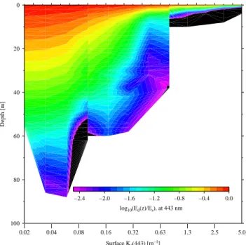
The combination of the sampling constraints described above with the characteristics of water masses and bottom topog-raphy led to the exploration of a large range of conditions in terms of water turbidity and optical complexity. This is illustrated in Fig. 2, which shows the exponential decrease of downward irradiance normalized to its value just below the sea surface, sorted as a function of the diffuse attenua-tion coefficient for downward irradiance at 443 nm, Kd(443)

(see Sect. 2.1 for determination of Kd). The right part of the

plot, for Kd(443) > ∼ 0.6 m−1, corresponds to sampling in

the two river transects (station numbers from 680 in the west Mackenzie transect and 394 to 398 for the east transect; see Fig. 1). At these very turbid stations, the one-percent light level (z1%)for λ = 443 nm is at depths from about 1 to 5 m.

At a few intermediate stations, where ∼ 0.3 m−1< Kd(443)

< ∼0.6 m−1, this depth is of about 20–30 m. For the clearest

stations (Kd(443) < ∼ 0.2 m−1), z1 %varies from about 50 to

70 m. The data set is therefore essentially made, on the one hand, of clear waters of the deep Beaufort Basin and shelf waters with water depths greater than about 50 m (17 sta-tions over a total of 36) and, on the other hand, of very turbid waters from the Mackenzie outflows (11 stations). Eight sta-tions represent intermediate situasta-tions, some of them being classified as “coastal”.

Four stations have been selected to illustrate in more de-tail the underwater light environments that were sampled dur-ing Malina Leg2b. The corresponddur-ing downward irradiance spectra at various depths, normalized to the maximum value found in the shallowest spectrum, are displayed in Fig. 3. They show, as expected, the progressive shift of the maxi-mum transmission from the blue wavelengths (λ ∼ 490 nm) for the clear station (Fig. 3b) to the green for mesotrophic sta-tions (Fig. 3b), and to the green and red for the highly turbid stations of the river transect (Fig. 3c and d). The underwa-ter environment at these turbid stations is nearly depleted of UV radiation, which is absorbed within the first meter (less than 1 % radiation for λ < 400 nm at a depth of 1 m). The

Ed peak due to Chl a fluorescence appears at the depth of

the deep chlorophyll maximum for the clearest station, i.e., at about 50 m (Fig. 3a), and, to lesser extent, at station 170

0 20 40 60 80 100 Depth [m] 0.02 0.04 0.08 0.16 0.32 0.63 1.3 2.5 5.0 Surface Kd(443) [m−1_] −2.4 −2.0 −1.6 −1.2 −0.8 −0.4 0.0 log10(Ed(z)/Es), at 443 nm 2013 Jun 05 14:35:58 Fig. 2

Fig. 2. Vertical profiles of the decimal logarithm of the downward

irradiance normalized to its value just below the sea surface. Data are sorted as a function of the Kd(443) value for the surface layer.

Discontinuities are due to sorting the profiles as a function of the surface Kdonly.

located near Cape Bathurst where moderate Chl a concen-trations were observed (i.e., 0.5 to 1.7 mg m−3)(Fig. 3b). At other stations, there is either not enough Chl a or too much of the light is absorbed in the blue-green by CDOM to produce a significant fluorescence signal.

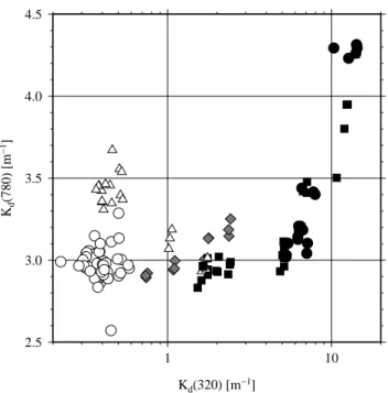
The large range of optical characteristics encountered dur-ing Malina Leg2b can actually be depicted by the relation-ship between the diffuse attenuation coefficient for down-ward irradiance (Kd) at the two extremes of the spectrum

sampled here, i.e., at 320 and 780 nm. The rationale for using these two values as a classification tool is fully ex-plored in the companion paper of this study (Hooker et al., 2013). Here it is used to show how the data set is distributed among different light regimes, and to identify stations clus-ters and assign them symbols that will be used from now on in this study to facilitate data interpretation. When plot-ting Kd(780) as a function of Kd(320) (Fig. 4), a first group

of stations clearly shows up with low Kd values for both

wavelengths. They correspond to the more offshore stations, and they will be identified by open circles. A number of sta-tions that would intuitively fall in the same category if they were classified on the basis of their geographical proximity with open-ocean stations actually separately appear in Fig. 4. They show low Kd(320) but moderate Kd(780) values. They

also correspond to clear waters but were characterized by the presence of an ice floe close to where the radiometry pro-files were performed. These “ice-edge” stations are identified

10−6 10−5 10−4 10−3 10−2 10−1 100 Normalized E d (λ ) 300 400 500 600 700 800 A Station 345−2 1 m 3 m 5 m 7 m 10 m 20 m 30 m 50 m 10−6 10−5 10−4 10−3 10−2 10−1 100 300 400 500 600 700 800 B Station 170−1 1 m 3 m 5 m 7 m 10 m 20 m 10−6 10−5 10−4 10−3 10−2 10−1 100 Normalized E d (λ ) 300 400 500 600 700 800 Wavelength [nm] C Station 693 1 m 3 m 5 m 7 m 10 m 20 m 10−6 10−5 10−4 10−3 10−2 10−1 100 300 400 500 600 700 800 D Station 398 Wavelength [nm] 1 m 3 m 2013 Jun 05 14:36:50 Fig. 3

Fig. 3. Example spectra of the downward irradiance at various depths and four stations as indicated. Values are normalized to the maximum

Edfound just below the sea surface.

by open triangles. Most of the stations corresponding to the two river transects have Kd(320) values greater than 3 m−1.

Therefore they very clearly separate from other stations (dark circles and squares). Stations of the northern part of the west-ern Mackenzie transect (640 to 680) represent an intermedi-ate situation (cluster of black squares for Kd(320) ∼ 2 m−1

and Kd(780) ∼ 3 m−1). Gray diamonds identify the coastal

stations.

3.3 Case-1/case-2 water classification

The irradiance reflectance at 560 nm, R(560), is plotted as a function of the Chl a concentration, Chl, in Fig. 5a. The theoretical maximum value of R(560) above which waters would belong to the sediment-dominated case-2 category (Morel and Prieur, 1977) has been computed from Chl a following Morel and B´elanger (2006) (continuous curve in Fig. 5a). Clearly, a large part of the Malina Leg2b data set is made of so-called case-2-S waters. As expected, these wa-ters essentially correspond to the two river transects and the

coastal stations, where water turbidity was high. A few of the open-ocean stations would also fall in the same category, at least with the criterion used here. It is known, however, that the theoretical threshold poorly performs for low Chl a and does not distinguish yellow-substance-dominated case-2 wa-ters (Morel and B´elanger, 2006). The ice-edge stations all fall below the theoretical line, which indicates that closeness of an ice floe would not enhance scattering in the green part of the spectrum, which is the parameter that essentially drives the theoretical threshold used here. Another possibility is that enhanced scattering is counterbalanced by enhanced absorp-tion in these particular situaabsorp-tions (see Sect. 3.3.2 in B´elanger et al., 2013).

Another look at the case-1/case-2 classification is given in Fig. 5b, where the ratio of remote sensing reflectances at 412 and 443, Rrs(412) / Rrs(443), is plotted as a function

of the Rrs(555) / Rrs(490) ratio (as in Lee and Hu, 2006; see

also Morel and Gentili, 2009). A monotonic relationship ex-ists between both ratios when they are determined from a case-1 water bio-optical model. Lee and Hu (2006) derived

2.5 3.0 3.5 4.0 4.5 Kd (780) [m −1 ] 1 10 Kd(320) [m−1] 2013 May 15 14:53:03 Fig. 4

Fig. 4. Kd(780) as a function of Kd(320). The grouping of points

shown here was used to group stations into different clusters as fol-lows: offshore clear-water stations (open circles), coastal stations (gray diamonds), the western Mackenzie transect (black squares), the eastern Mackenzie transect (black circles), and ice-edge stations (open triangles).

such a relationship from the Chl-based bio-optical model of Morel and Maritorena (2001) (MM01). The corresponding curve is superimposed on the Malina data points in Fig. 5b. Case-1 water stations should be distributed within ±10 % of this theoretical line (see Fig. 1 in Lee and Hu, 2006), which is not the case here. The entire data set, on the con-trary, falls well below the average curve and outside of the

±10 % variability, which indicates a much lower than ex-pected Rrs(412) / Rrs(443) ratio. This is a clear indication of

an excess of absorption by CDOM.

Therefore, although the more offshore stations of Malina Leg2b can be ascribed to the case-1 water category when looking at a criterion essentially based on scattering (Fig. 5a), none of the stations would belong to this category when the classification is based on the relative proportion of CDOM with respect to scattering (or Chl a).

3.4 Spectral characteristics

A few stations have been selected as exemplary of spectral shapes present in our data set. The corresponding spectra of normalized Rrs and Kd’s are displayed in Fig. 6a and b,

re-spectively, for stations 394–398 (east transect), 380 (coastal), 320, 340 and 360 (open-ocean clear waters), and 460 and 760 (ice-edge stations). For the river stations, extremely low Rrs

in the UV bands, around 5 × 10−5sr−1, combined with large values in the red part of the spectrum (about 2 × 10−2sr−1)

0.01 0.1 R(560) 0.01 0.1 1 10 TChla [mg m−3_] A Case II Case I 0.0 0.5 1.0 1.5 2.0 Rrs (412) / R rs (443) 0.0 0.5 1.0 1.5 2.0 R_rs(555) / R_rs(490) B Case I 2013 May 15 14:53:07 Fig. 5

Fig. 5. (A) Irradiance reflectance at 560 nm, R(560), as a

func-tion of the Chl a concentrafunc-tion. The curve corresponds to the the-oretical limit between case-1 and case-2 waters, computed from Chl a following Morel and B´elanger (2006). (B) Rrs(412)/Rrs(443)

as a function of Rrs(555)/Rrs(490). The solid line corresponds to

Eq. (2a) in Lee and Hu (2006), and the dashed curves to ±10 % around this line.

make Rrs varying over about three decades. The Rrs values

for open-ocean and coastal stations vary over slightly more than two decades. The Kdvalues in the UV bands can be as

high as 20 m−1in the innermost part of the Mackenzie River mouth. In the visible spectral domain, the lowest values are of about 0.035 m−1. They expectedly correspond to the blue bands (490 nm in particular) of the open-ocean stations.

The case-1/case-2 delineation examined in Fig. 5 is insuf-ficient to fully characterize the optical regimes. It cannot, in particular, indicate whether or not the waters classified here as case-1 have similar spectral characteristics as case-1 wa-ters of other oceanic areas. It has already been shown that optical properties of low-chlorophyll clear waters can sig-nificantly vary at a given Chl a concentration (Morel et al., 2007a; Brown et al., 2008). Therefore, the spectral shape of

1e−05 0.0001 0.001 0.01 Normalized R rs [sr −1 ] 300 400 500 600 700 800 Wavelength [nm] A 0.01 0.1 1 10 Kd (λ ) [m −1 ] 300 400 500 600 700 800 Wavelength [nm] B 2013 May 15 14:53:17 Fig. 6 Fig. 6. Example Rrs(A) and Kd(B) spectra, for stations 320, 340

and 360 (open waters), 235 and 460 (ice edge), 380 (coastal), and 394–398 (eastern Mackenzie transect). The open diamonds show modeled values from Morel and Maritorena (2001).

offshore stations in the Beaufort Sea have been compared to the prediction of the MM01 bio-optical model, in order to see how this particular sea behaves with respect to the mean conditions encountered in the world ocean. The model was fed with the average Chl a concentration and Sun zenith an-gle of the 3 stations shown in Fig. 6 (Chl a = 0.05 mg m−3,

θs=62◦). The resulting Rrsand Kdare displayed in Fig. 6a

and b as open diamonds connected by a dotted line (note that the spectral range of the model is limited to 350–700 nm). They show a close coincidence with the measured spectra for all spectral bands from 490 to 700 nm, but a much higher

Rrs and much lower Kd in the near UV and blue parts of

the spectrum than what was measured in the Beaufort Sea during Malina Leg2b (by about ±50 % at 443 nm, and by a factor of about 2 at 412 nm, for instance). What is referred to as open-ocean clear water here for the Beaufort Sea is ac-tually much less blue than what can be found in other low-chlorophyll waters around the world. A similar depression of Rrsbelow 450 nm has been reported for the Beaufort Sea

by previous authors (Wang and Cota, 2003; Matsuoka et al., 2007; B´elanger et al., 2007). A higher absorption by CDOM at a given Chl a concentration is likely responsible for this difference. This can be illustrated by computing the 8 factor from Morel and Gentili (2009), which expresses the excess or deficit in CDOM absorption as compared to what the Morel and Maritorena (2001) model would predict for a given Chl a concentration. With a ratio R(412)/R(443) of about 0.95 and a ratio R(490)/R(555) of about 3.5, as derived from the spectra shown in Fig. 6, and for Chl a = 0.05 mg m−3, the 8 factor would be close to 5 (see Fig. 2b in Morel and Gen-tili, 2009). This is a clear indication that CDOM absorption is much higher in the clear waters of the Beaufort Sea than it is elsewhere (see also B´elanger et al., 2013, and references therein).

The spectra identified by open triangles in Fig. 6 cor-respond to two of the ice-edge stations. The surface Chl a concentration for these two stations is in the same range as for the three open-ocean stations also displayed in Fig. 6 (open circles), namely values from 0.035 to 0.05 mg(Chl) m−3. Their Rrs spectra differ for wavelengths

lower than ∼ 500 nm, however, with lower values for the ice-edge stations. A much more significant difference is observed for the Kdspectra, by at least a factor of two, and not only for

blue bands but across the entire spectrum. The enhanced par-ticulate absorption in the top 2 m of the water column iden-tified by B´elanger et al. (2013) is likely responsible for this increase in Kd. In addition, the spectral shapes of the two

ice-edge Kdspectra are different, indicating that the

proxim-ity of ice does not always lead to the same perturbation of optical properties. It may depend on the proximity of the ice edge, on the thickness of the ice sheet, the mixing conditions prior to measurement and on the chemical composition of the material that is released in the water when ice melts.

3.5 Bio-optical relationships

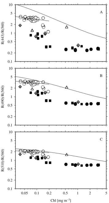
Radiometry measurements are not only used for character-ization of the underwater light field. They are also largely used as inputs to bio-optical models aiming at quantify-ing geophysical parameters such as the Chl a concentration. We have accordingly examined whether existing bio-optical models that were developed for global ocean case-1 waters could apply to the clear waters of the Beaufort Sea, either in their forward mode (i.e., deriving AOPs from Chl a) or in their inverse forms to derive Chl a from combinations – usu-ally ratios – of AOPs. We used the MM01 as a typical model

0.1 0.2 0.5 1 2 5 10 R(443)/R(560) A 0.1 0.2 0.5 1 2 5 10 R(490)/R(560) B 0.1 0.2 0.5 1 2 5 10 R(510)/R(560) 0.05 0.1 0.2 0.5 1 2 5 Chl [mg m−3_] C 2013 May 15 14:55:36 Fig. 7

Fig. 7. Reflectance ratios for the wavelengths indicated, as a

func-tion of the Chl a concentrafunc-tion. The thick solid curves show mod-eled values from Morel and Maritorena (2001). The thin solid curves are linear fits using the log-transformed data, for the clear-water stations only.

for case-1 waters. The results are displayed on the three pan-els of Fig. 7, where three reflectance ratios are plotted as a function of Chl a, using either the field data (symbols) or the model (solid curve). None of the three reflectance ratios are appropriately reproduced by the model. The predicted aver-age of the reflectance ratio is closer to the field values when using the 510-to-560 band ratio, but still with a significant overestimation (15–20 %). For the open-ocean stations the measured reflectance ratios are actually close to being insen-sitive to Chl a when it is lower than about 0.15 mg m−3. This is illustrated by plotting the regression curve obtained on the

log-transformed data, which shows a slope close to 0 (from

−0.19 in Fig. 7a to −0.08 in Fig. 7c). Clearly, the MM01 model cannot be used to predict reflectance ratios from Chl a in clear waters of the Beaufort Sea. Because the MM01 model is the basis for the OC4Me “satellite chl” maximum-band-ratio algorithm (Morel et al., 2007b), using the latter to derive Chl a from the reflectance ratios is also invalid, regardless of whether these ratios are obtained from field or satellite remote sensing observations (OC4Me was con-ceived to apply to observations from the European Medium Resolution Imaging Spectrometer – MERIS – ocean colour sensor). This comment can be actually extended to any simi-larly derived algorithm such as the OC4-like algorithms used by the NASA Sea-viewing Wide Field-of-view Sensor (Sea-WiFS) and Moderate Resolution Imaging Spectroradiome-ter (MODIS) ocean color missions. As a consequence, ac-curately deriving Chl a in these clear waters from current ocean color remote sensing algorithms based on global data sets seems illusory. The Chl retrievals obtained via such al-gorithms are shown in Fig. 8, for the OC4Me (Morel et al., 2007) and GSM (Garver and Siegel, 1997; Maritorena et al., 2002) global algorithms, and for an algorithm locally tuned to the southeast Beaufort Sea waters (Ben Mustapha et al., 2012). The GSM algorithm performs better than the OC4Me because it allows for a varying CDOM component, whereas OC4Me assumes proportionality between Chl and CDOM absorption. Both algorithms overestimate the field determinations, however. The local and empirical algorithm performs clearly better for Chl > ∼ 0.2 mg m−3, yet it largely underestimates Chl in clear waters.

For the river transects, the reflectance ratios are also close to being insensitive to Chl a when it is greater than about 0.2 mg m−3. This is rather expected, however, because op-tical properties at these stations are essentially under the influence of sediments. However, when the three panels in Fig. 7 are redrawn as a function of SPM instead of Chl a (not shown), a similar grouping of stations appears, with thresh-olds of about 0.5 and 2 g m−3, respectively, below and above which the reflectance ratios little vary. Therefore, two optical regimes exist in the Beaufort Sea, inside which neither Chl a nor SPM have a significant influence on the reflectance ra-tios, at least in the wavelength range examined here (440 to 560 nm). So, deriving these quantities from AOP ratios (or other AOP combinations) probably necessitates embracing a broader spectral range.

Therefore, a thorough exploration of the relationships be-tween AOPs or ratios of AOPs, and either IOPs or geophysi-cal quantities such as particulate absorption, Chl a and SPM, has been performed. Considering the high value we got for the 8 parameter (see above), absorption by CDOM has been considered as well. Because the range of optical regimes was large in the Leg2b data set, and because those waters that would belong to the case-1 category when using a Chl a cri-terion actually behave differently from average models, the logic was to search for bio-optical relationships that would

0.01 0.02 0.05 0.1 0.2 0.5 1 2 5 10 Chl, model [mg m −3 ] 0.010.02 0.05 0.1 0.2 0.5 1 2 5 Chl, field [mg m−3_] A OC4Me 0.01 0.02 0.05 0.1 0.2 0.5 1 2 5 10 Chl, model [mg m −3] 0.010.02 0.05 0.1 0.2 0.5 1 2 5 Chl, field [mg m−3_] B GSM 0.01 0.02 0.05 0.1 0.2 0.5 1 2 5 Chl, model [mg m −3] 0.010.02 0.05 0.1 0.2 0.5 1 2 5 Chl, field [mg m−3_] C BM12 2013 May 30 18:12:45 Fig. 8 Fig. 8. Chl concentrations retrieved from (A) OC4Me, (B) GSM and

(C) Ben Mustapha et al. (2012) algorithms (see text), as a function

of the Chl value determined from field samples.

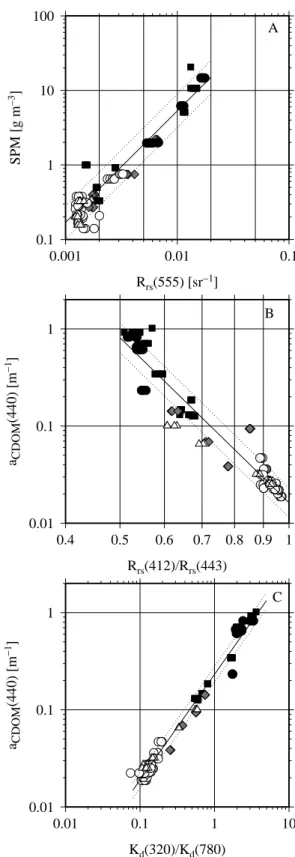
0.1 1 10 100 SPM [g m −3 ] 0.001 0.01 0.1 Rrs(555) [sr−1] A 0.01 0.1 1 aCDOM (440) [m −1 ] 0.4 0.5 0.6 0.7 0.8 0.9 1 Rrs(412)/Rrs(443) B 0.01 0.1 1 aCDOM (440) [m −1 ] 0.01 0.1 1 10 Kd(320)/Kd(780) C 2013 May 15 14:55:48 Fig. 9 Fig. 9. Bio-optical relationships in the Malina Leg2b data set. Solid

curves are regression fits on the log-transformed data, and the dotted curves show the RMSE around the regressions (A) Rrs(555) nm as a

function of SPM concentration, (B) ratio of Rrs(412) to Rrs(443) as

a function of CDOM absorption at 440 nm, and (C) ratio of Kd(320)

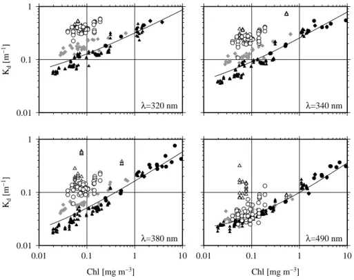
0.01 0.1 1 Kd [m −1] λ=320 nm λ=340 nm 0.01 0.1 1 Kd [m −1] 0.01 0.1 1 10 Chl [mg m−3_] λ=380 nm 0.01 0.1 1 10 Chl [mg m−3_] λ=490 nm 2013 Jun 05 14:33:50 Fig. 10

Fig. 10. Kdas a function of Chl a, and for selected wavelengths as indicated (redrawn from Morel et al., 2007a, with addition of the data

from Malina Leg2b). The open symbols are for the Malina Leg2b clear-water stations, the gray symbols for the Mediterranean Sea, and the black symbols for South Pacific data. The continuous black curve represents the MM01 prediction.

encompass the entire range of conditions encountered here, recognizing however that they could not be as accurate as specific relationships that would be established on more ho-mogeneous subsets of data (e.g., only the clear-water sta-tions). The latter might show a better predictive accuracy lo-cally, yet they would have less general applicability.

This exercise revealed only three relationships valid for the entire data set and with an acceptable predictive accu-racy. They emphasize the SPM concentration as a function of

Rrs(555) (Fig. 9a), the CDOM absorption as a function of the

Rrs(412) / Rrs(443) ratio (Fig. 9b), and the CDOM absorption

as a function of the Kd(320) / Kd(780) ratio (Fig. 9c). The

relative predictive skill of the linear regressions is given here as the root mean square error (RMSE) of the log-log regres-sion. It is of about 50 % for derivation of SPM directly from

Rrs(555), of about 35 % for derivation of aCDOM(440) from

the Rrs(412) / Rrs(443) ratio, and of about 20 % for derivation

of aCDOM(440) from the Kd(320) / Kd(780) ratio. The latter

provides an interesting opportunity to derive aCDOM from

field radiometry only, which is of great help, considering the difficulty in accurately measuring aCDOMfrom field samples.

This relationship would not, however, be of great help in a remote sensing context where spectral Kdvalues have to be

determined indirectly from the sole quantity amenable to re-mote sensing, i.e., from spectral Rrs. The less-accurate yet

still-acceptable relationship shown in Fig. 9b would have to be used from satellite Rrs.

4 Discussion

It has been previously reported that the contribution of ab-sorption by CDOM relative to other absorbing material, in particular phytoplankton, is higher in the absorption budget of Arctic waters than in other parts of the world ocean (Pe-gau, 2002; Hill, 2008; Matsuoka et al., 2007, 2011; B´elanger et al., 2008, 2013; Ben Mustapha et al., 2012). Our re-sults (Figs. 5, 6) confirm these specific characteristics, which were also quantified through the calculation of the 8 pa-rameter from Morel and Gentili (2009). A synthetic view of the anomalously high attenuation in the UV and blue parts of the spectrum is provided in Fig. 10 (Kd as a

func-tion of Chl a), where the Kdvalues for clear waters of

Ma-lina Leg2b (open symbols) are superimposed on values from other oceans (gray and black symbols), as redrawn from Morel et al. (2007a). This figure clearly shows that the Beau-fort Sea clear waters have more absorption in the UV-blue for given low Chl a levels than any other clear waters we have previously sampled (when “clear water” is defined with respect to Chl a).

Among Malina’s objectives is the determination of net pri-mary production (NPP) in the Arctic from ocean color re-mote sensing observations. When doing so using so-called “satellite-chl” algorithms (Carr et al., 2006), one undergoes three main initial steps: (1) deriving surface Chl a from spectral Rrs (O’Reilly et al., 1998; Morel et al., 2007b),

0 20 40 60 80 100 120

Modeled depth of the DCM [m]

0 20 40 60 80 100 120

Measured depth of the DCM [m]

2013 May 15 14:55:51 Figure 11

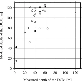
Fig. 11. Predicted versus measured depth of the deep chlorophyll

maximum (DCM). Stations from the two river transects are ex-cluded from this comparison because they do not exhibit a DCM (stations 395 to 398, and 691 to 695). 0 5 10 15 20 25

% of surface irradiance at DCM depth

300 400 500 600 700 Wavelength [nm] 320 110 760 460 2013 May 15 14:55:52 Fig. 12

Fig. 12. Percentage of surface irradiance that reaches the depth

of the deep chlorophyll maximum (DCM). The percentage is de-termined either from the radiometry profiles (black dots) or from MM01 (dashed curves) fed with the measured vertical Chl a pro-file.

(2) estimating the depth profile of Chl a from its surface value (e.g., Morel and Berthon, 1989; Uitz et al., 2006), and (3) propagating incoming spectral irradiance using this Chl a vertical profile and a bio-optical model (MM01 for instance). Subsequent steps that are not considered here are the estima-tion of absorpestima-tion of the available light at any depth by phy-toplankton, and the transfer of the absorbed energy to photo-synthesis (through parameterization of the production versus irradiance curve).

1 10 100

Modeled depth of the 1% light level [m]

1 10 100

Measured depth of the 1% light level [m]

1 10 100

Modeled depth of the 10% light level [m]

1 10 100

Measured depth of the 10% light level [m]

2013 May 15 14:56:02 Figure 13

Fig. 13. Predicted (MM01) versus measured depth of the 1 % (top)

and 10 % (bottom) light levels. Symbols are as for previous figures, i.e., circles for open-ocean stations and triangles for ice-edge sta-tions. Pink, blue, green, red, and black symbols are for λ = 380, 443, 555, 670 nm and PAR, respectively.

The inappropriateness of current bio-optical algorithms re-ported here (Fig. 7) shows that step 1 would be wrongly achieved if using them, resulting in a large overestimation of Chl a (Fig. 8). Solving this issue requires using either locally tuned Chl a algorithms or NPP algorithms that are not Chl-based (e.g., Hirawake et al., 2012; Mouw and Yoder, 2005). Combining the retrieval of non-water absorption, at,

aCDOM (Matsuoka et al., 2013) might help in providing an

estimate of particulate absorption (ap=at−aCDOM), from

which phytoplankton absorption, aϕ, could be derived (e.g.,

Bricaud and Stramski, 1990) and used as an input to aϕ-based

models.

Step 2 would also be wrongly achieved because the Chl a vertical profile is not correctly reproduced by existing pa-rameterizations, which in particular largely overestimate the depth of the deep chlorophyll maximum (DCM). This is il-lustrated here using the Morel and Berthon (1989) model, which predicts the shape of the vertical Chl a profile from knowledge of the surface value only. For clear-water sta-tions, the overestimation is generally at least by a factor of two (Fig. 11). Using such a parameterization would largely underestimate the contribution of the DCM to the integrated NPP over the productive column.

Finally, step 3 (irradiance propagation) would also be per-formed incorrectly (see Fig. 6). This is further illustrated here by comparing the amount and spectral composition of downward irradiance at the measured depth of the DCM. This composition is determined either from the Ed(λ)

spec-tra measured at the DCM depth or from specspec-tra modeled from MM01 when fed with the measured Chl a(z) profile (Fig. 12). This comparison clearly shows that there is much less radiation in the near UV and blue part of the spectrum that reaches the DCM in clear waters of the Beaufort Sea than what the model predicts. This further illustrates the strong dimming effect of CDOM absorption in these waters. An-other consequence of this effect is that the depth of the pro-ductive layer is much reduced as compared to what the model would predict. This is shown in Fig. 13, where the measured and modeled depths of the 1 % and 10 % light levels are com-pared for different wavelengths and also for PAR. As a con-sequence, conclusions about the importance of the DCM in the NPP budget of Arctic waters may need to be revised in light of these very peculiar attenuation properties. That as-pect was ignored in Arrigo et al. (2011), for instance. Com-pensating effects may occur among the various parameteriza-tions, however, eventually decreasing errors in NPP predic-tions as compared to what can be expected from the separate examination of the steps outlined above. NPP cannot be reli-ably estimated, however, by hoping that such effects indeed occur, which advocates for developing Arctic-specific NPP models.

Another overarching objective of the Malina program is to address interannual to decadal changes of the phytoplank-ton communities in the Arctic, in particular by assessing Chl a concentrations from ocean color remote sensing ob-servations. The results reported here confirm, however, that remote sensing of Chl a is likely infeasible in the clear wa-ters of the Arctic using conventional techniques based on absorption in the blue part of the spectrum, because of the dominance of absorption by CDOM in this spectral domain. Maximum-band-ratio algorithms such as the OC4-type algo-rithms (O’Reilly et al., 2000) or simpler relationships such

as those shown here (Fig. 9) are more likely to be used for remote sensing of CDOM absorption. The difficulty in get-ting Chl a from ocean color could be solved by exploiget-ting other parts of the spectrum, e.g., the red (Dall’Olmo et al., 2006; Shen et al., 2010). This could prove useful for moder-ately to highly turbid waters but not for clear waters, where the marine reflectance in the red is extremely small (Fig. 6a). Our AOP data set is likely one of the most extensive for the Arctic, and relationships were derivable that can provide regional-scale distribution of CDOM from satellite remote sensing, assuming that the upstream issue of atmospheric corrections has been solved. This data set is, however, still restricted to the Beaufort Sea in August. Additional data are therefore desirable if one aims at a comprehensive view of optical properties in the entire Arctic Ocean, at least during the periods of the year when ocean color remote sensing is possible.

Acknowledgements. We are grateful to the captain and crew of the Canadian Icebreaker CCGS Amundsen. This study was conducted as part of the Malina Scientific Program funded by ANR (Agence nationale de la recherche), INSU-CNRS (Institut national des sciences de l’univers – Centre national de la recherche scientifique), CNES (Centre national d’´etudes spatiales) and ESA (European Space Agency). We thank Jos´ephine Ras for the HPLC pigment analyses and David Doxaran for providing the SPM data. Edited by: K. Suzuki

The publication of this article is financed by CNRS-INSU.

References

Arrigo, K. R., Matrai, P. A., and Van Dijken G. L.: Primary produc-tivity in the Arctic Ocean: impacts of complex optical properties and subsurface chlorophyll maxima on large-scale estimates, J. Geophys. Res., 116, C11022, doi:10.1029/2011JC007273, 2011. Austin, R. W.: The remote sensing of spectral radiance from below the ocean surface, in: Optical Aspects of Oceanography, edited by: Jerlov, N. G. and Nielsen, E. S., Academic Press, London, 317–344, 1974.

Babin, M., Stramski, D., Ferrari, G. M., Claustre, H., Bricaud, A., Obolensky, G., and Hoepffner, N.: Variations in the light absorp-tion coefficients of phytoplankton, nonalgal particles, and dis-solved organic matter in coastal waters around Europe, J. Geo-phys. Res., 108, 3211, doi:10.1029/2001JC000882, 2003. B´elanger, S., Ehn, J., and Babin, M.: Impact of Sea Ice on

the Retrieval of Water-leaving Reflectance, Chlorophyll a Concentration and Inherent Optical Properties from Satel-lite Ocean Color Data, Remote Sens. Environ., 111, 51–68, doi:10.1016/j.rse.2007.03.013, 2007.

B´elanger, S., Babin, M., and Larouche, P.: An empirical ocean color algorithm for estimating the contribution of chro-mophoric dissolved organic matter to total light absorption in optically complex waters, J. Geophys. Res., 113, C04027, doi:10.1029/2007JC004436, 2008.

B´elanger, S., Cizmeli, S. A., Ehn, J., Matsuoka, A., Doxaran, D., Hooker, S., and Babin, M.: Light absorption and partitioning in Arctic Ocean surface waters: impact of multi year ice melting, Biogeosciences Discuss., 10, 5619–5670, doi:10.5194/bgd-10-5619-2013, 2013.

Ben Mustapha, S., B´elanger, S., and Larouche, P.: Evaluation of ocean color algorithms in the southeastern Beaufort Sea, Cana-dian Arctic: New parameterization using SeaWiFS, MODIS and MERIS spectral bands, Can. J. Remote Sens., 54, 535–556, 2012. Bricaud, A. and Stramski, D.: Spectral absorption coefficients of living phytoplankton and nonalgal biogenous matter: A compar-ison between the Peru upwelling area and the Sargasso Sea, Lim-nol. Oceanogr., 35 , 562–582, 1990.

Brown, C. A., Huot, Y., Werdell, P. J., Gentili, B., and Claustre, H.: The origin and global distribution of second order variabil-ity in satellite ocean color and its potential applications to al-gorithm development, Remote Sens. Environ., 112, 4186–4203, doi:10.1016/j.rse.2008.06.008, 2008.

Brunelle, C. B., Larouche, P., and Gosselin, P.: Variability of phy-toplankton light absorption in Canadian Arctic seas, J. Geophys. Res., 117, C00G17, doi:10.1029/2011JC007345, 2012. Carr, M.-E.,Friedrichs, M. A. M., Schmeltz, M., Ait´e, M. N.,

An-toine, D., Arrigo, K. R., Asanuma, I., Aumont, O., Barber, R., Behrenfeld, M., Bidigare, R., Buitenhuis, E., Campbell, J., Ciotti, A., Dierssen, H., Dowell, M., Dunne, J., Esaias, W., Gentili, B., Groom, S., Hoepffner, N., Hishisaka, J., Kameda, T., LeQu´er´e, C., Lohrenz, S., Marra, J., M´elin, F., Moore, K., Morel, A., Reddy, T., Ryan, J., Scardi, M., Smyth, T., Turpie, K., Tilstone, G., Waters, K., Yamanaka, Y.: A comparison of global estimates of marine primary production from ocean color, Deep-Sea Res., Pt. II, 53, 741–770, 2006.

Dall’Olmo, G., Gitelson, A. A., Rundquist, D. C. Leavitt, B. Bar-row, T. J., and Holz, C.: Assessing the potential of SeaWiFS and MODIS for estimating chlorophyll concentration in turbid pro-ductive waters using red and near-infrared bands, Remote Sens. Environ., 96, 176–187, 2006.

Doxaran, D., Ehn, J., B´elanger, S., Matsuoka, A., Hooker, S., and Babin, M.: Optical characterisation of suspended particles in the Mackenzie River plume (Canadian Arctic Ocean) and implica-tions for ocean colour remote sensing, Biogeosciences, 9, 3213– 3229, doi:10.5194/bg-9-3213-2012, 2012.

Eastman, R. and Warren, S. G.: Interannual variations of Arctic cloud types in relation to sea ice, J. Climate, 23, 4216–4232, doi:10.1175/2010JCLI3492.1, 2010.

Garver, S. A. and Siegel, D. A.: Inherent optical property inversion of ocean color spectra and its biogeochemical interpretation 1. time series from the Sargasso Sea, J. Geophys. Res., 102, 18607– 18625, 1997.

Gordon, H. R. and Clark, D. K.: Clear water radiances for atmo-spheric correction of coastal zone color scanner imagery, Appl. Optics, 20, 4175–4180, 1981.

Hill, V.: The Impacts of Chromophoric Dissolved Organic Material on Surface Ocean Heating in the Chukchi Sea, J. Geophys. Res., 113, doi:10.1029/2007JC004119, 2008.

Hirawake, T., Shinmyo, K., Fujiwara, A., and Saitoh, S.: Satellite re-mote sensing of primary productivity in the Bering and Chukchi Seas using an absorption-based approach, ICES J. Mar. Sci., 69, 1194–1204, doi:10.1093/icesjms/fss111, 2012.

Hooker, S. B.: The telescoping mount for advanced solar technolo-gies (T-MAST), in: Advances in Measuring the Apparent Optical Properties (AOPs) of Optically Complex Waters, edited by: Mor-row, J. H., Hooker, S. B., Booth, C. R., Bernhard, G., Lind, R. N., and Brown, J. W., NASA Tech. Memo. 2010, 215856, NASA Goddard Space Flight Center, Greenbelt, Maryland, 80 pp., 2010. Hooker, S. B. and Brown, J. W.: Processing of Radiometric Obser-vations of Seawater using Information Technologies (PROSIT): In-Water User Manual, NASA Tech. Memo., NASA Goddard Space Flight Center, Greenbelt, Maryland, in preparation, 2013. Hooker, S. B., Zibordi, G., Berthon, J.-F., D’Alimonte, D., Mari-torena, S., McLean, S., and Sildam, J.: Results of the Second Sea-WiFS Data Analysis Round Robin, March 2000 (DARR-30 00), NASA Tech. Memo. 2001–206892, Vol. 15, edited by: Hooker, S. B. and Firestone, E. R., NASA Goddard Space Flight Center, Greenbelt, Maryland, 71 pp., 2001.

Hooker, S. B., Van Heukelem, L., Thomas, C. S., Claustre, H., Ras, J., Barlow, R., Sessions, H., Schluter, L., Perl, J., Trees, C., Stuart, V., et al.: The second SeaWiFS HPLC Analysis Round-Robin Experiment (SeaHARRE-2), in Technical Memorandum NASA/TM-2005-212787, 112 pp., NASA Goddard Space Flight Center, Greenbelt, MD, 2005.

Hooker, S. B., Morrow, J. H., and Matsuoka, A.: Apparent optical properties of the Canadian Beaufort Sea – Part 2: The 1 % and 1 cm perspective in deriving and validating AOP data products, Biogeosciences, 10, 4511–4527, doi:10.5194/bg-10-4511-2013, 2013.

Joint Global Ocean Flux Stud: JGOFS Core Measurements Proto-cols, JGOFS Report No. 6, Scientific Committee on Oceanic Re-search, Bergen, Norway, 40 pp., 1991.

Lee, Z. and Hu, C.: Global distribution of Case-1 waters: An anal-ysis from SeaWiFS measurements, Remote Sens. Environ., 101, 270–276, 2006.

Maritorena, S., Siegel, D. A., and Peterson, A.: Optimization of a Semi-Analytical Ocean Colour Model for Global Scale Applica-tions, Appl. Optics, 41, 2705-2714, 2002.

Matsuoka, A., Huot, Y., Shimida, K., Saitoh, S.-I., and Babin, M.: Bio-optical characteristics in the Western Arctic Ocean: Impli-cations for ocean color algorithms, Can. J. Remote Sens., 33, 503–518, 2007.

Matsuoka, A., Larouche, P., Poulin, M., Vincent, W., and Hattori, H.: Phytoplankton community adaptation to changing light lev-els in the southern Beaufort Sea, Canadian Arctic, Estuar. Coast. Shelf S., 82, 537–546, 2009.

Matsuoka, A., Hill, V., Huot, Y., Babin, M., and Bricaud, A.: Sea-sonal variability in the light absorption coefficient of phytoplank-ton, non-algal particles, and colored dissolved organic matter in western Arctic waters: parameterization of the individual com-ponents of absorption for ocean color applications, J. Geophys. Res., 116, C02007, doi:10.1029/2009JC005594, 2011.

Matsuoka, A., Bricaud, A., Benner, R., Para, J., Semp´er´e, R., Prieur, L., B´elanger, S., and Babin, M.: Tracing the transport of colored dissolved organic matter in water masses of the Southern Beau-fort Sea: relationship with hydrographic characteristics, Biogeo-sciences, 9, 925–940, doi:10.5194/bg-9-925-2012, 2012.

Matsuoka, A., Hooker, S. B., Bricaud, A., Gentili, B., and Babin, M.: Estimating absorption coefficients of colored dissolved or-ganic matter (CDOM) using a semi-analytical algorithm for southern Beaufort Sea waters: application to deriving concentra-tions of dissolved organic carbon from space, Biogeosciences, 10, 917–927, doi:10.5194/bg-10-917-2013, 2013.

Maykut, G. A. and Grenfell, T. G.: The spectral distribution of light beneath first-year ice in te Arctic ocean, Limnol. Oceanogr., 20, 554–563, 1975.

Mitchell, B. G.: Predictive bio-optical relationships for polar oceans and marginal ice zones, J. Marine Syst., 3, 91–105, 1992. Mobley, C. D.: Estimation of the remote-sensing reflectance from

above-surface measurements, Appl. Optics, 38, 7442–7455, 1999.

Morel, A. and B´elanger, S.: Improved Detection of turbid waters from Ocean Color information, Remote Sens. Environ., 102, 237–249, 2006.

Morel, A. and Berthon, J. F.: Surface pigments, algal biomass pro-files, and potential production of the euphotic layer: Relation-ships reinvestigated in view of remote-sensing applications, Lim-nol. Oceanogr., 34, 1545–1562, 1989.

Morel, A. and Gentili, B.: Diffuse reflectance of oceanic waters. 2. Bidirectional aspects, Appl. Optics, 32, 6864–6872, 1993. Morel, A. and Gentili, B.: Diffuse reflectance of oceanic waters. 3.

Implication of bidirectionality for the remote-sensing problem, Appl. Optics, 35, 4850–4862, 1996.

Morel, A. and Gentili, B.: A simple band ratio technique to quantify the colored dissolved and detrital organic material from ocean color remotely sensed data, Remote Sens. Environ., 113, 998– 1011, doi:10.1016/j.rse.2009.01.008, 2009.

Morel, A. and Maritorena, S.: Bio-optical properties of oceanic wa-ters: A reappraisal, J. Geophys. Res., 106, 7763–7780, 2001. Morel, A. and Prieur, L.: Analysis of variations in ocean color,

Lim-nol. Oceanogr., 22, 709–722, 1977.

Morel, A., Claustre, H., Antoine, D., and Gentili, B.: Natural vari-ability of bio-optical properties in Case 1 waters: attenuation and reflectance within the visible and near-UV spectral domains, as observed in South Pacific and Mediterranean waters, Biogeo-sciences, 4, 913–925, doi:10.5194/bg-4-913-2007, 2007a. Morel, A., Huot, Y., Gentili, B., Werdell, P. J., Hooker, S. B., and

Franz B. A.: Examining the consistency of products derived from various ocean color sensors in open ocean (Case 1) waters in the perspective of a multi-sensor approach, Remote Sens. Environ., 111, 69–88, 2007b.

Mouw, C. and Yoder, J. A.: Primary production calculations in the Mid-Atlantic Bight, including effects of phytoplankton commu-nity size structure, Limnol. Oceanogr., 50, 1232–1243, 2005. Mueller, J. L.: Overview of measurement and data analysis protocol,

in: Ocean Optics Protocols for Satellite Ocean Color Sensor Vali-dation, Revision 2, NASA Tech. Memo. 2000–209966, edited by: Fargion, G. S. and Mueller, J. L., NASA Goddard Space Flight Center, Greenbelt, Maryland, 87–97, 2000.

Mueller, J. L.: Overview of measurement and data analysis proto-cols, in: Ocean Optics Protocols for Satellite Ocean Color Sensor Validation, Revision 3, Volume 1, NASA Tech. Memo. 2002– 210004/Rev3–Vol1, edited by: Mueller, J. L. and Fargion, G. S., NASA Goddard Space Flight Center, Greenbelt, Maryland, 123– 137, 2002.

Mueller, J. L.: Overview of measurement and data analysis meth-ods, in: Ocean Optics Protocols for Satellite Ocean Color Sen-sor Validation, Revision 4, Volume III: Radiometric Measure-ments and Data Analysis Protocols, NASA Tech. Memo. 2003– 211621/Rev4 Vol.III, edited by: Mueller, J. L., Fargoin, G. S., and McClain, C. R., NASA Goddard Space Flight Center, Green-belt, Maryland, 1–20, 2003.

Mueller, J. L. and Austin, R. W.: Ocean optics protocols for Sea-WiFS validation, NASA Tech. Memo. 104566, Vol. 5, edited by: Hooker, S. B. and Firestone, E. R., NASA Goddard Space 30 Flight Center, Greenbelt, Maryland, 43 pp., 1992.

Mueller, J. L. and Austin, R. W.: Ocean optics protocols for Sea-WiFS validation, Revision 1, NASA Tech. Memo. 104566, Vol. 25, edited by: Hooker, S. B., Firestone, E. R., and Acker, J. G., NASA Goddard Space Flight Center, Greenbelt, Maryland, 66 pp., 1995.

Mueller, J. L. and Morel, A.: Fundamental definitions, relation-ships and conventions, in: Ocean Optics Protocols for Satel-lite Ocean Color Sensor Validation, Revision 4, Volume I: Ra-diometric Measurements and Data Analysis Protocols, NASA Tech. Memo. 2003–211621/Rev4–Vol.I, edited by: Mueller, J. L., Austin, R. W., Morel, A., Fargion, G. S., and McClain, C. R., 5 NASA Goddard Space Flight Center, Greenbelt, Maryland, 11–30, 2003.

O’Reilly, J. E., Maritorena, S., Mitchell, B. G., Siegel, D. A., Carder, K. L., Garver, S. A., Kahru, M., and McClain, C.: Ocean color chlorophyll algorithms for SeaWiFS, J. Geophys. Res., 103, 24937–24953, 1998.

O’Reilly, J. E., Maritorena, S., O’Brien, M. C., Siegel, D. A., Toole, D., Menzies, D., Smith, R. C., Mueller, J. L., Mitchell, B. G., Kahru, M., Chavez, F. P., Strutton, P., Cota, G. F., Hooker, S. B., McClain, C. R., Carder, K. L., Muller-Karger, F., Harding, L., Magnuson, A., Phinney, D., Moore, G. F., Aiken, J., Arrigo, K. R., Letelier, R., and Culver, M.: SeaWiFS Postlaunch Calibra-tion and ValidaCalibra-tion Analyses, Part 3. NASA Tech. Memo. 2000-206892, Vol. 11, edited by: Hooker, S. B. and Firestone, E. R., NASA Goddard Space Flight Center, 49 pp., 2000.

Pegau, W. S.: Inherent optical properties of the central Arctic surface waters, J. Geophys. Res., 107, 8035, doi:10.1029/2000JC000382, 2002.

Pegau, W. S., Gray, D., and Zaneveld, J. R. V.: Absorption and at-tenuation of visible and near infrared light in water: dependence on temperature and salinity, Appl. Optics, 36, 6035–6046, 1997. Preisendorfer, R. W.: Application of radiative transfer theory to light measurements in the sea, Monogr. Int. Union Geod. Geophys. Paris, 10, 11-30, 1961.

Schuur, E. A. G., Bockheim, J., Canadell, J. G., Euskirchen, E., Christopher, B., Goryachkin, S.V., Hagemann, S., Kuhry, P., Lafleur, P. M., Lee, H., Mazhitova, G., Nelson, F. E., Rinke, A., Romanovsky, V. E., Shiklomanov, N., Tarnocai, C., Venevsky, S., Vogel, J. G., and Zimov, S. A.: Vulnerability of Permafrost Carbon to Climate Change: Implications for the Global Carbon Cycle, BioSci., 58, 701–714, doi:10.1641/B580807, 2008. Shen, F., Zhou, Y., Li, D., Zhu, W., and Salama, Mhd., S.:

Medium resolution imaging spectrometer (MERIS) estimation of chlorophyll-a concentration in the turbid sediment-laden waters of the Changjiang (Yangtze) Estuary, Int. J. Remote Sens., 31, 4635–4650, 2010.