HAL Id: hal-02934576
https://hal.sorbonne-universite.fr/hal-02934576
Submitted on 9 Sep 2020
HAL is a multi-disciplinary open access
archive for the deposit and dissemination of
sci-entific research documents, whether they are
pub-lished or not. The documents may come from
teaching and research institutions in France or
abroad, or from public or private research centers.
L’archive ouverte pluridisciplinaire HAL, est
destinée au dépôt et à la diffusion de documents
scientifiques de niveau recherche, publiés ou non,
émanant des établissements d’enseignement et de
recherche français ou étrangers, des laboratoires
publics ou privés.
Case study of multi-temperature coronal jets for
emerging flux MHD models
Reetika Joshi, Ramesh Chandra, Brigitte Schmieder, Fernando
Moreno-Insertis, Guillaume Aulanier, Daniel Nóbrega-Siverio, Pooja Devi
To cite this version:
Reetika Joshi, Ramesh Chandra, Brigitte Schmieder, Fernando Moreno-Insertis, Guillaume Aulanier,
et al.. Case study of multi-temperature coronal jets for emerging flux MHD models. Astronomy
and Astrophysics - A&A, EDP Sciences, 2020, 639, pp.A22. �10.1051/0004-6361/202037806�.
�hal-02934576�
A&A 639, A22 (2020) https://doi.org/10.1051/0004-6361/202037806 c R. Joshi et al. 2020
Astronomy
&
Astrophysics
Case study of multi-temperature coronal jets for emerging flux
MHD models
?
Reetika Joshi
1,2, Ramesh Chandra
2, Brigitte Schmieder
1,3,4, Fernando Moreno-Insertis
5,6, Guillaume Aulanier
1,
Daniel Nóbrega-Siverio
7,8, and Pooja Devi
21 Observatoire de Paris, LESIA, UMR8109 (CNRS), 92195 Meudon Principal Cedex, France
e-mail: [email protected], [email protected]
2 Department of Physics, DSB Campus, Kumaun University, Nainital 263 001, India
3 Centre for Mathematical Plasma Astrophysics, Dept. of Mathematics, KU Leuven, 3001 Leuven, Belgium
4 SUPA School of Physics and Astronomy, University of Glasgow, Glasgow G12 8QQ, UK
5 Instituto de Astrofisica de Canarias, Via Lactea, s/n, 38205 La Laguna, Tenerife, Spain 6 Department of Astrophysics, Universidad de La Laguna, 38200 La Laguna, Tenerife, Spain
7 Rosseland Centre for Solar Physics, University of Oslo, PO Box 1029, Blindern 0315, Oslo, Norway 8 Institute of Theoretical Astrophysics, University of Oslo, PO Box 1029, Blindern 0315, Oslo, Norway
Received 24 February 2020/ Accepted 11 May 2020
ABSTRACT
Context.Hot coronal jets are a basic observed feature of the solar atmosphere whose physical origin is still actively debated.
Aims.We study six recurrent jets that occurred in active region NOAA 12644 on April 4, 2017. They are observed in all the hot filters of AIA as well as cool surges in IRIS slit–jaw high spatial and temporal resolution images.
Methods.The AIA filters allow us to study the temperature and the emission measure of the jets using the filter ratio method. We studied the pre-jet phases by analysing the intensity oscillations at the base of the jets with the wavelet technique.
Results.A fine co-alignment of the AIA and IRIS data shows that the jets are initiated at the top of a canopy-like double-chambered structure with cool emission on one and hot emission on the other side. The hot jets are collimated in the hot temperature filters, have high velocities (around 250 km s−1) and are accompanied by cool surges and ejected kernels that both move at about 45 km s−1. In the pre-phase of the jets, we find quasi-periodic intensity oscillations at their base that are in phase with small ejections; they have a period of between 2 and 6 min, and are reminiscent of acoustic or magnetohydrodynamic waves.
Conclusions.This series of jets and surges provides a good case study for testing the 2D and 3D magnetohydrodynamic emerging flux models. The double-chambered structure that is found in the observations corresponds to the regions with cold and hot loops that are in the models below the current sheet that contains the reconnection site. The cool surge with kernels is comparable with the cool ejection and plasmoids that naturally appears in the models.
Key words. Sun: activity – Sun: magnetic fields – Sun: oscillations
1. Introduction
Solar coronal jets are detected throughout the entire solar cycle in a wide wavelength range, from X-rays (Shibata et al. 1992) to the extreme ultraviolet (EUV; Wang et al. 1998;
Alexander & Fletcher 1999; Innes et al. 2011; Sterling et al. 2015; Chandra et al. 2015; Joshi et al. 2017a). Many jets are seen as collimated plasma material that flows with high veloc-ity along open magnetic field lines. Other interesting ejec-tions are cool surges, which emerge in the form of unwrinkled threads of dark material in Hα (Roy 1973;Mandrini et al. 2002;
Uddin et al. 2012; Li et al. 2016), and sprays, which are very fast ejections that generally originate in active region filaments (Warwick 1957; Tandberg-Hanssen et al. 1980; Pike & Mason 2002; Martin 2015). Some surges are closely related to hot jets (Schmieder et al. 1988;Canfield et al. 1996). Solar coronal jets are observed in active (Sterling et al. 2016; Chandra et al. 2017; Joshi & Chandra 2018) and quiet regions (Hong et al. 2011; Panesar et al. 2016). Their physical parameters such as height (1–50 × 104km), lifetime (tens of minutes to one
? Movies are available athttps://www.aanda.org
hour), width (1–10 × 104km), and velocity (100–500 km s−1)
have been studied by many authors (Shimojo et al. 1996;
Savcheva et al. 2007; Nisticò et al. 2009; Filippov et al. 2009;
Joshi et al. 2017b).
Magnetic reconnection is believed to trigger the activation of the jet phenomenon according to different theoretical mod-els (Yokoyama & Shibata 1995; Archontis et al. 2004, 2005;
Pariat et al. 2015). Reconnection is the process of restructuring the magnetic field lines and can occur in 2D (Filippov 1999;
Pontin et al. 2005) or in 3D configurations (Démoulin & Priest 1993; Filippov 1999; Longcope et al. 2003; Priest & Pontin 2009; Masson et al. 2009). In a 2D magnetic null-point con-figuration, magnetic field lines contained in a plane and with opposite orientations approach eachother across an X-point and instantaneously change connectivity; the result are hybrid field lines that are expelled away from the X-point, typically with velocities of about the Alfvén speed. In 3D there is a whole vari-ety of possible patterns (e.g. spine-fan, torsional, or separator reconnection pattern); in many cases, the underlying structure is known as a fan-spine configuration around a central null-point. The field lines from inside the fan surface are joined to open field lines from just outside with ensuing connectivity change.
Changes in the remote connectivity of magnetic field lines may also take place in regions with strong spatial gradients of the field components that are called quasi-separatrix layers (QSLs;
Mandrini et al. 2002).
Magnetic reconnection can take place as a result of a pro-cess of magnetic flux emergence from the low solar atmo-sphere or interior. In typical magnetic flux emergence processes, the emerging magnetised plasma interacts with the pre-existing ambient coronal magnetic field, thus providing a favourable con-dition for magnetic reconnection, and therefore for the occur-rence of solar jets. The observations indicate that the expan-sion of the region in which the magnetic flux emerges leads to reconnection with the ambient quasi-potential field and magnetic cancellation (Gu et al. 1994; Schmieder et al. 1996; Liu et al. 2011; Guo et al. 2013). A number of numerical models have simulated this process (see e.g. Yokoyama & Shibata 1996;
Archontis et al. 2004; Moreno-Insertis et al. 2008; Török et al. 2009; Moreno-Insertis & Galsgaard 2013; Archontis & Hood 2013; Nóbrega-Siverio et al. 2016; Ni et al. 2017). In the model by Moreno-Insertis et al. (2008), in particular, a split-vault structure is clearly shown to form below the jet, and it contains two chambers: the chamber containing previ-ously emerged loops with a decrease in volume, and the chamber containing reconnected loops with a increase in vol-ume as a result of reconnection. This structure is also con-firmed in radiation-magnetohydrodynamic (MHD) simulations by Nóbrega-Siverio et al. (2016). The observations that moti-vated those models were either X-ray jets observed by Hinode (Moreno-Insertis et al. 2008), or cool surges observed in chro-mospheric lines and bright bursts in transition region lines (Nóbrega-Siverio et al. 2017), but these models have not yet been compared with simultaneously observed hot jets and cool surges. On the other hand, for another category of MHD mod-els, the important mechanism that drives the jet onset is not the emerging flux itself, but the injection of helicity through photo-spheric motions (Pariat et al. 2015,2016); see further references in the review byRaouafi et al.(2016). Shear and/or twist motions at the base of the closed non-potential region below a preexisting null-point induces reconnection with the ambient quasi-potential flux and initiates untwisting or helical jets (Pariat et al. 2015;
Török et al. 2016). In some of these MHD models that are based on the loss of equilibrium through twisting motions, the thermal plasma parameters of the jets are not directly considered, but are suggested by correspondence parameters such as the plasma β (Pariat et al. 2016).
The observational analysis from previous studies has revealed that the jet evolution might be preceded by some wave-like or oscillatory disturbances (Pucci et al. 2012;Li et al. 2015;
Bagashvili et al. 2018). Pucci et al. (2012) analysed the X-ray jets observed by Hinode November 2−4, 2007 and found that most of the jets are associated with oscillations of the coronal emission in bright points (for a recent review of coronal bright points, seeMadjarska 2019) at the base of the jets. They con-cluded that the pre-jet oscillations are the result of the change in area or temperature of the pre-jet activity region. Recently, a statistical analysis of pre-jet oscillations of coronal hole jets has been carried out byBagashvili et al.(2018). They reported that 20 out of 23 jets in their study were preceded by pre-jet intensity oscillations some 12−15 min before the onset of the jet. They tentatively suggested that these quasi-periodic inten-sity oscillations may be the result of MHD wave generation through rapid temperature variations and shear flows associated with local reconnection events (Shergelashvili et al. 2006).
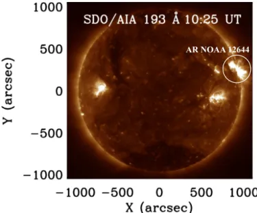
AR NOAA 12644
Fig. 1.Full-disc image of the Sun on April 4, 2017. The solar jets were ejected from active region NOAA 12644 that is shown by the white cir-cle at the west limb.
Here, we found a series of jets observed in the hot EUV channels of Atmospheric Imaging Assembly (AIA;Lemen et al. 2012) on board the Solar Dynamics Observatory (SDO;
Pesnell et al. 2012) as well as in cool temperatures with the Interface Region Imaging Spectrograph (IRIS;De Pontieu et al. 2014) slit-jaw images. The jets were ejected from active region NOAA 12644 on April 4, 2017; on that date, the region was located at the west limb (N13W91) (Fig. 1). When it passed through the central meridian, this region had shown high jet activity alongside episodes of emerging magnetic flux (Ruan et al. 2019). Its location at the limb in the present obser-vations allows us to visualise the structure of the brightenings from the side and thus facilitates the comparison with the MHD jet models, which motivates our research.
The layout of the paper is as follows. We present the observa-tions and kinematics of jets and identify the reconnected struc-tures in Sect.2. Pre-jet oscillations are reported in Sect.3. We discuss our results in Sect.4. We conclude that this series of jet and surge observations obtained with a high spatial and tempo-ral resolution match important aspects of the expected behaviour predicted by MHD models of emerging flux. We are able to iden-tify a candidate location for the current sheet and reconnection site, and we follow the evolution of the cool surge and hot jets with individual blob ejections. This is a clear case study for 2D and 3D MHD models where flux emergence is the trigger of the jet.
2. Jets
2.1. Observations
We selected six jet eruptions that occurred in active region NOAA 12644 at the western solar limb on April 4, 2017. We used data from SDO/AIA and IRIS. AIA observes the full Sun in seven UV and EUV wavelengths (94 Å, 131 Å, 171 Å, 193 Å, 211 Å, 304 Å, and 335 Å) with a pixel size and temporal cadence of 000. 6 and 12 s. We aligned the complete data set using the
drot_map routine. For the bad pixel correction, we processed the level 1 AIA data to level 1.5 using the code aia_prep.pro. These
codes are available in SolarSoftWare (SSW) on the IDL plat-form. IRIS simultaneously provides spectra and images of the photosphere, chromosphere, transition region, and corona that cover a temperature range between 5000 K and 10 MK. Slit-jaw images (SJI) are obtained in four different passbands with a high spatial and temporal resolution of 000. 16 pixel−1 and 1.5 s. The
IRIS data set includes two transition region lines (C II 1330 Å, Si IV 1400 Å), one chromospheric line (Mg IIk 2796 Å), and one photospheric passband (in the Mg II wing around 2830 Å). We took the IRIS level 1.5 data from the data archive1. The level 1.5 data were corrected for dark current, and we removed the far-UV (Ffar-UV) background data by iris_prep.pro in SSWIDL. The IRIS target was pointed towards active region NOAA 12644 at the western limb with a field of view of 12600× 11900 between
11:05:38 UT and 17:58:35 UT. For our current study, we used the SJIs in the C II and Mg II k bandpasses obtained with a cadence of 16 s. The SJIs picture the chromospheric plasma around 104K.
2.2. Characteristics of the jets
On April 4, 2017, active region jets were observed at the limb between 02:30 and 17:10 UT with AIA. The movies in di ffer-ent wavelengths of AIA (131 Å, 171 Å, and 304 Å) reveal two sites of plasma ejections (jets) along the limb. First, a northern site ([92100, 26400]), where the jets are straight and their base is located behind the limb and hence concealed by it. Second, a site south of the field of view ([93100, 25500]) in which the jet bases
are above the limb. Therefore we here studied the six main jets that originated in the southern site and occurred after 10:00 UT. Five of them were also observed by IRIS, but the first occurred before the IRIS observations.
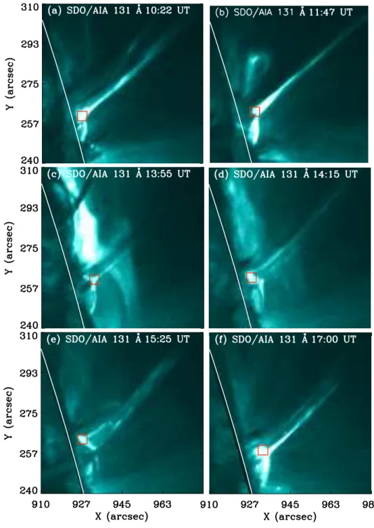
These jets reached an altitude between 30 and 70 Mm; their recurrence period was around 80 min, with the exception of two jets that were separated by only 15 min. The movies also show many small jets that reach less than 10 Mm height both before and in between the main jets. The jets observed in AIA 131 Å are shown in Figs.2a–f and in an accompanying animation (MOV1). The first main jet, jet1, reaches its peak at ≈10:22 UT with an average speed of 210 km s−1 (panel a). Jet2 (panel b) starts at
11:45 UT and reaches its maximum extent at ≈11:47 UT. In the movie (MOV1) we note a large filament eruption located on the northern site of the jets that erupts at ≈13:30 UT and falls back after reaching its maximum height. Moreover, the jet and fila-ment are not associated with each other. Jets3 and 4 (panel b and c, respectively) reach their maximum altitude at 13:55 UT and 14:15 UT, respectively. Jet5 (panel e) erupts with a broader base and reaches its maximum height at ≈15:25 UT. The jet base along a bright loop is fast extended laterally. Jet6 (panel f) is ejected at ≈16:57 UT. A second instance of filament eruption is observed during the peak phase of jet6, which starts again at the same location as the first. In this case, the erupted filament mate-rial seems to merge later with the jet matemate-rial and is ejected in the same direction. However, here the jet is not launched by the filament eruption because it is not at the jet base location.
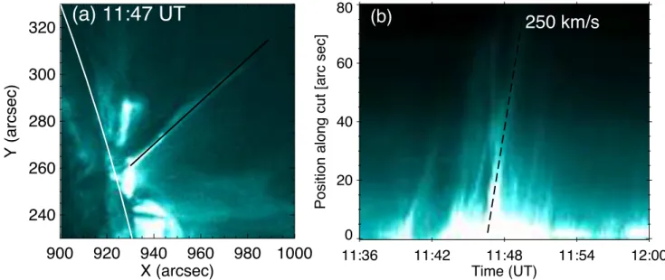
We computed various physical parameters: height, width, lifetime, and speed of these jets. To do this, we used the AIA 131 Å data. For the velocity calculation, we calibrated the height-time of each jet in AIA 131 Å by fixing a slit in the mid-dle of the jet plasma flow and calculated the average speed in the flow direction. An example of the height-time calculation is
1 http://iris.lmsal.com/search
shown in Fig.3for jet2. All computed physical parameters are listed in Table1. The maximum height, average speed, width, and lifetime of the observed jets vary in the ranges ≈30−80 Mm, 200−270 km s−1, 1−7 Mm, and 2−10 min.
Jets2–6were also observed by IRIS in two wavelength pass-bands: CII (top row of Fig.4) and MgII k (bottom row). The high spatial resolution of IRIS allowed us to make a clear iden-tification of what looks like a null-point structure at a height of ≈6 Mm. The CII filter shows bright loops above a bright half-dome in the northern site of the jet footpoints. In the Mg II filter, the northern part of the dome is also bright. We find jet strands throughout the northern side of the dome, like a collection of sheets. We discuss these jet strands, which are cool jets or surges with a lower velocity, in Sect.2.4. In AIA 131 Å all the jets show a bright area that might correspond to a current sheet (CS), pos-sibly containing a null-point, with underlying bright loops shap-ing a dome (Fig.2). However, the bright dome and loops are located on the southern side of the tentative CS, whereas the bright loops in IRIS C II are on its northern side. In the fol-lowing, when we refer to observations of this candidate CS and possible null-point we sometimes call them “the null point” for simplicity even though there is clearly no way in which a zero-point of the magnetic field (or the intensity of the electric current) in these temperatures might be detected with current observational means. Moreover, in all the hot channels of AIA (131 Å, 193 Å, 171 Å, and 211 Å) and IRIS C II and Mg II SJIs, the jets have an anemone (so-called Eiffel-tower or inverted-Y) structure, with a loop at the base and elongated jet arms (see Figs.2and4), as reported in previous events (Nisticò et al. 2009;
Schmieder et al. 2013; Liu et al. 2016). In AIA 131 Å the ten-tative CS and the jet spine move in the south–west direction between the first and last eruption (Fig.2). More precisely, by following the motion of the point with maximum intensity, we determined a drift of 5 arcsec in less than 6 h.
2.3. Temperature and emission measure analysis
We investigated the distribution of the temperature and emission measure (EM) at the jet spire for all jet events. We performed the differential emission measure (DEM) analysis with the regu-larised inversion method introduced byHannah & Kontar(2012) using six AIA channels (94 Å, 131 Å, 171 Å, 193 Å, 211 Å, and 335 Å). After this process, we obtained the regularised DEM maps as a function of temperature. We used a temperature range from log T (K)= 5.5 to 7 with 15 different bins of width ∆ log T = 0.1. We calculated the EM and lower limit of the electron density in the jet spire using ne=
√
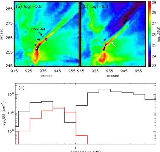
E M/h, where h is the jet width, assum-ing that the fillassum-ing factor equals unity. These EM values were obtained by integrating the DEM values over the temperature range log T (K)= 5.8 to 6.7. We chose a square box to measure the EM and density at the jet spire and at the same location before the jet activity for each jet. The example for the DEM analysis of jet2is presented in Fig.5, which represents the DEM maps at two different temperatures, log T(K) = 5.8 (panel a) and 6.3 (panel b), at 11:45 UT. We investigated the temperature variation at the jet spire during the jet and pre-jet phase. During the pre-jet phase for jet2, the log EM and the electron density values were 27.3 and 2 × 109cm−3, whereas for the jet phase, the values were 28.1 and 8.6×109cm−3, respectively. Thus, during the jet evolution the EM
value increased by over one order of magnitude and the electron density increased by a factor three at the jet spire. The EM and density values increased during the jet phase in all six jets. The values for all jets are listed in Table1.
Fig. 2. Six solar jets (jets1–6) in AIA 131 Å filter. The red square in each panel shows the position at which the pre-jet oscillations are measured. The limb is indicated by the white circle in each panel.
2.4. Identification of observed structural elements
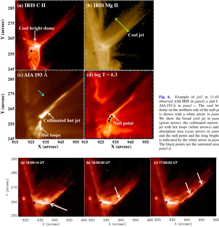
In Sect.2.2we discussed the morphology of the jets observed with AIA and IRIS. The region below the jet, as seen in different wavelengths, has a remarkably clear structure, resembling the structures discussed in theoretical models in the past years. For identification with previous theoretical work, in Fig. 6 several structural elements are indicated for the case of the jet2 obser-vations. In IRIS CII (Fig. 6, panel a), the brightenings below the jet delineate a double-chambered vault structure, with the main brightening being located in the northern part of the base of the jet. Only narrow loops are seen above the southern part of the vault in this wavelength. In the other chromospheric line, IRIS Mg II, we see (panel b) roughly the same scenario, although the general picture is rather fuzzier. The jet, in particular, is no longer narrow, but is formed by parallel strands issuing from the
edge of the northern part of the vault, similar to a comb (Fig.6
panel b). The assumption of a double-vault structure below the jet is reinforced in the two hot-plasma observations (AIA 193 Å, panel c) and the temperature map obtained through the DEM analysis explained in the previous section (panel d). In these two panels, the southern loops are shown to be bright and hot struc-tures, and the same applies to the point right at the base of the jet, where the temperature reaches 106K. Additionally, bright
kernels sometimes move along the jets and are more clearly vis-ible in jets4–6. An example of brightening kernels that move along jet6 in IRIS CII is presented in Fig.7. We computed the velocities of the kernels and find that they are comparable to the mean velocities of the cool jet (45 km s−1). The time between the ejection of two kernels is shorter than 2 min.
The structural elements described above seem to correspond to various prominent features in the numerical 3D models of
11:36
11:42
11:48
11:54
12:00
Time (UT)
0
20
40
60
80
Position along cut [arc sec]
250 km/s
(b)
900
920
940
960
980
1000
X (arcsec)
240
260
280
300
320
Y (arcsec)
(a) 11:47 UT
Fig. 3.Example of a time-slice analysis of jet1 that we used for velocity and height calculations in AIA 131 Å. Panel a: the solid black line is the slit location, which we used to create the height-time plot (b).
Table 1. Physical parameters of the six hot jets.
Jet Jet start Jet peak Max Average T EM Oscillation
no. time time height speed (1028 period
(UT) (UT) (Mm) (km s−1) (MK) cm−5) (min)
1 10:15 10:22 80 210 1.4 1.4 6.0 2 11:46 11:47 50 245 1.8 1.9 1.5 3 13:54 13:55 40 265 1.4 1.5 2.5 4 14:12 14:15 50 250 1.8 1.1 2.0 5 15:23 15:25 55 235 1.8 1.3 4.0 6 16:57 17:00 70 220 1.8 2.0 2.5
Moreno-Insertis et al. (2008) and Moreno-Insertis & Galsgaard
(2013), or in the more recent 2D models ofNóbrega-Siverio et al.
(2016,2018), all of which studied in detail the consequences in the atmosphere of the emergence of magnetised plasma from below the photosphere. The bright and hot plasma apparent in the obser-vations at the base of the jet can be identified with the null-point and CS structures in these simulations (see the scheme in Fig.8, right panel): the collision of the emerging magnetised plasma with the pre-existing coronal magnetic system leads, when the mutual orientation of the magnetic field is sufficiently different, to the for-mation of an elongated CS harbouring a null-point, and it leads to reconnection. As a next step in the pattern identification, the hot plasma loops apparent in the southern vault in the AIA 193 Å image and the temperature panels of Fig.6should correspond to the hot post-reconnection loop system in the numerical models (as apparent in Figs. 3 and 4 inMoreno-Insertis et al. 2008, or in
Moreno-Insertis & Galsgaard 2013). On the other hand, the north-ern vault appears dark in AIA 193 Å and has lower temperatures in the DEM analysis. This region might then correspond to the emerged plasma vault underlying the CS in the numerical models: the magnetised plasma in that region is gradually brought toward the CS, where the magnetic field is reconnected with the coronal field.
Additional features in the observation that fit this identifica-tion are listed below.
(a) As time proceeds, the northern chamber decreases while the southern chamber grows. In our observations in the begin-ning phase of the jets (e.g. jet2 at 11:30 UT), the area of the northern and southern vaults is 1.4×10¹⁸and 1.16×1018cm2, respectively, and during the jet phase (11:47 UT), they become 1.05×10¹⁸and 2.2×1018cm2, respectively. This
sug-gests that while the reconnection occurs, the emerging vol-ume decreases, whereas the reconnected loop domain grows, as in the emerging flux models (Moreno-Insertis et al. 2008;
Moreno-Insertis & Galsgaard 2013; Nóbrega-Siverio et al. 2016).
(b) One main item for identifying the observation with the flux emergence models is the possibility that we also observe a wide, cool, and dense plasma surge that is ejected in the neighbourhood of the vault and jet complex (see the movie in C II attached as MOV2). This wide laminar jet is observed in the Mg II IRIS filter as an absorption sheet parallel to the hot jet in AIA 193 Å. The evolution of the cool mate-rial at both sides of the hot jet in the IRIS Mg II chan-nel is presented in Fig.9, and the leading edge of the cool part is indicated by red stars. The cool ejection is gener-ally less collimated than the hot jet and is seen to first rise and then fall, similar to classical Hα surges. The veloci-ties measured along the cool sheet of plasma in Mg II are ≈ 45 km s−1. The ejection of cool material next to the hot
jets is a robust feature in different flux emergence mod-els (Yokoyama & Shibata 1996;Moreno-Insertis et al. 2008;
Nishizuka et al. 2008; Moreno-Insertis & Galsgaard 2013;
MacTaggart et al. 2015;Nóbrega-Siverio et al. 2016,2017,
2018). The cool plasma in the models consists of matter that has gone over from the emerged plasma domain to the sys-tem of reconnected open coronal field lines without passing near the reconnection site, that is, just by flowing, because of flux freezing, alongside the magnetic lines that are recon-nected at a higher level in the corona. All these models report velocities that match the observed value quoted above very well.
(c) The observed kernels in Fig.7might be plasmoids created in the CS during the reconnection process. In some of the flux emergence models just discussed, plasmoids are created in
Fig. 4.IRIS observed the active region from 11:05 UT to 17:58 UT. It covers five jets in our present analysis in CII (top) and MgII k (bottom) lines. The black points in the top panels are produced by extreme saturation, which we used for a better visibility of jets.
Fig. 5. Top: two maps of the active region jet2 at 11:45 UT at two di ffer-ent temperatures (log T= 5.8 and 6.3). The blue square in panel a shows the location we used for the emission anal-ysis at the jet spire. The black arrow in panel a indicates a weak EM region that we call the cool jet, and the white arrow in panel b shows the hot jet. Bottom: the red line shows the temper-ature at the location of the blue box in panel a before the first jet ejec-tion on April 4, 2017, and the black line shows the temperature of the solar active region jet at 11:45 UT.
the CS domain (see e.g.Moreno-Insertis & Galsgaard 2013), and they are hurled out of the sheet probably via the melon-seed instability (Nóbrega-Siverio et al. 2016), even though they are not seen to reach the jet region. Observational evi-dences of the formation of plasmoids in this kind of scenario have been found byRouppe van der Voort et al.(2017). On
the other hand, in the 2D jet model by Ni et al. (2017), plasmoids are created in the reconnection site and maintain their identity when they rise along the jet spire, possibly because of the higher resolution afforded by the advanced mesh refinement used in the model; this is in agreement with the behaviour noted in our observations and in the
(c) AIA 193
Å
(a) IRIS C II
(b) IRIS Mg II
(d) log T = 6.3
915 925 935 945 955 915 925 935 945 955 245 255 265 275 285 245 255 265 275 285X (arcsec)
X (arcsec)
Y
(ar
cs
ec
)
Y
(ar
cs
ec
)
Collimated hot jet
Null point
Hot loops
Cool jet
Cool bright dome
Fig. 6. Example of jet2 at 11:45 UT observed with IRIS in panels a and b and AIA 193 Å in panel c. The cool bright dome on the northern side of the null-point is shown with a white arrow in panel a. We show the broad cool jet in panel b (green arrow), the collimated narrow hot jet with hot loops (white arrows) and the absorption area (cyan arrow) in panel c, and the null-point and the long bright CS is indicated by the white arrow in panel d. The black points are the saturated areas in panel d.
(a) 16:59:14 UT (b) 16:59:30 UT (c) 17:00:03 UT
Fig. 7.Kernels of brightening that move along jet6 observed in the IRIS SJI in the CII wavelength range (see the white arrows). The kernels might correspond to untwisted plasmoids.
previous observations ofZhang & Ji(2014) andZhang et al.
(2016) mentioned in the introduction. Plasmoids are also generated in the model byWyper et al. (2016), which is a result of footpoint driving of the coronal field rather than flux emergence from the interior. On the other hand, the for-mation of the kernels might follow the development of the Kelvin–Helmholtz instability (KHI). The KHI can be pro-duced when two neighbouring fluids flow in same direction with different speeds (Chandrasekhar 1961). This instabil-ity may develop following the shear between the jet and its surroundings. For details about this sort of process in
jets and coronal mass ejections (CMEs), see the review by
Zhelyazkov et al.(2019).
(d) The main brightening at the top of the two vaults appears systematically to change position in the observations. There is a shift in the south–west direction as time advances, and the same displacement is apparent in AIA 131 Å (see Figs.2
and4); this might indicate the motion of the reconnection site. This type of observation is also reported in the study ofFilippov et al.(2009). This shift may be used to compare with the drift of the null-point position detected in the MHD models.
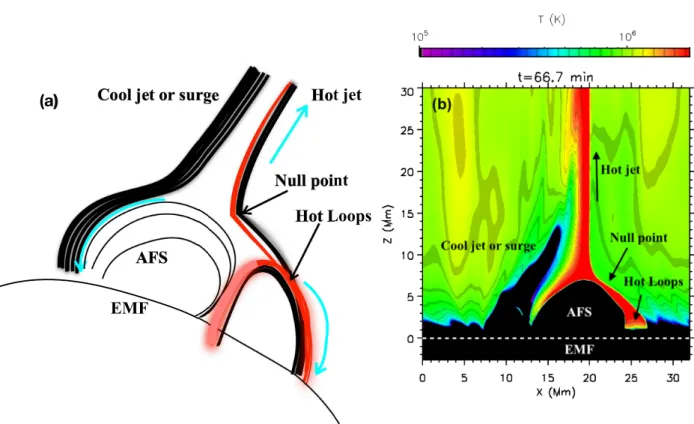
(a)
Cool jet or surge
Hot jet
Hot Loops
EMF
AFS
Null point
Fig. 8.Panel a: schematic view of the 3D jet derived fromMoreno-Insertis et al.(2008), showing the location of the null-point, the cool surge, and the hot loops next to the AFS. The cyan arrows indicate the flow direction. The red lines indicate hot plasma. The black lines are magnetic field lines. Panel b: temperature map of one of the numerical experiments byNóbrega-Siverio et al.(2017,2018) showing the hot jet and the cool surge (an animation of this panel is availableonline). In both panels, the region of the convection zone where the new magnetic flux has emerged (EMF) is also indicated.
⋆
⋆
⋆
⋆
⋆
⋆
Fig. 9.Evolution of cool plasma material on both sides of the hot jet (jet2) in the IRIS MgII wavelength. The red star shows the leading edge of the cool material that is ejected with an average speed of 45 km s−1.
(e) We also note a significant rise of the brighter point (null-point) between different jet events. The rise of the reconnec-tion site as the jet evolureconnec-tion advances has been found in the MHD emerging flux models ofYokoyama & Shibata(1995) andTörök et al. (2009). In our case, it may be because the reconnection process causes a displacement of the null-point and jet spine in each jet event. In this way, the next jet event occurs in a displaced location as compared with the previ-ous jet. This might indicate that the magnetic field configura-tion has some reminiscences of the earlier reconnecconfigura-tion and behaves in the same manner afterwards. Another possible
reason for this shifting might be that it is a result of the inter-action between different QSLs, as suggested byJoshi et al.
(2017b). However, because of the limb location of the active region, we were unable to compute the QSL locations here.
3. Oscillations before the jet activity
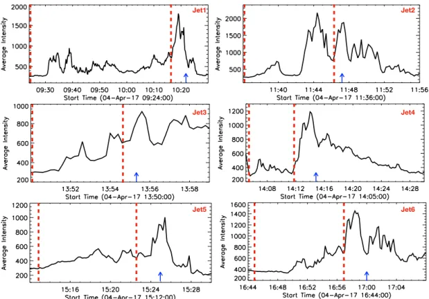
In Sect.2.2we reported that before and in between the six main jets, we also observed many small jet-like ejections, with lengths shorter than 10 Mm. Moreover, the AIA 131 Å movie clearly
Jet1 Jet2
Jet3 Jet4
Jet5 Jet6
Fig. 10.Intensity distribution during pre-phase of recurrent jets at the base of each jet in AIA 131 Å. The location of the jet base of each jet is displayed in Fig.2(see the red squares). In each panel, the blue arrow indicates the peak phase of the main jet. The small intensity peaks before each main jet are related to small jet ejections (10 Mm height) from the same location. The two vertical dashed red lines in each panel show the duration of the pre-jet intensity oscillation that is used for the wavelet analysis.
shows many episodic brightenings related to the small jets. In this section we investigate different properties of these features, such as the periodicity. To this end, we selected a square of size 4 × 4 arcsec at the base of the jets where the intensity is high-est in the AIA 131 Å data, as shown in Fig.2, and calculated the mean intensity inside the square in the AIA 131 Å channel. We computed the relative intensity variation at the base after normal-isation by the quiet-region intensity. We find that the oscillations start at the jet base some 5−40 min before the main jet activity. Figure10shows the intensity distribution at the jet base for all the jets before and during the jet eruption, and the pre-jet phase. The starting and peak time of the main jets are also indicated. The maximum of the brightening at the jet base does not always coincide exactly with the start of the jet or with the maximum extension time. In most cases, the maximum brightening occurs before the peak time of the jets by a few minutes. For the smaller jets it is nearly impossible to compute the delay between bright-enings and jets. They appear to be in phase with the accuracy of the measurements.
To calculate the time period of these pre-jet oscillations, we applied a wavelet analysis technique. For the significance of time periods in the wavelet spectra, we took a significance test into account, and levels higher than or equal to 95% were labelled as real. The significance test and the wavelet analysis technique are well described byTorrence & Compo(1998). The cone-of-influence (COI) regions make an important background for the edge effect at the start and end point of the time range (Tian et al. 2008;Luna et al. 2017). The wavelet analysis of the intensity fluctuation at the jet base shows that the oscillation period for these pre-jet intensities varies between 1.5 min and 6 min; the current values obtained are presented in the last
col-umn of Table 1. An example of the wavelet spectrum for the pre-jet activity for jet2 is presented in Fig.11a. The COI region is the outer area of the white parabolic curve. The global wavelet spectrum in panel b shows the distribution of power spectra over time. Bagashvili et al. (2018) investigated the intensity at the base of several jets issued from a coronal hole and obtained sim-ilar results concerning the periodicity and duration of the oscil-lations.
4. Discussion and conclusion
We presented observations of the structure, kinematics, and pre-jet intensity oscillations of six main pre-jets that occurred on April 4, 2017, in active region NOAA 12644. The discussion was based on the observational data from AIA and IRIS. A brief summary of our main results is listed below.
1. All the jets show pre-jet intensity oscillations at their base, accompanied by smaller jets. The oscillation period ranges from 1.5 to 6 min.
2. The jets are issued from a canopy-like structure with two vaults delineated by the brightenings seen in the different wavelengths. One of the vaults harbours hot loops, as seen in the EUV AIA filters and also in the IRIS C II wavelength. The hot jets are accompanied by laminar cool surge-like jets visible in IRIS Mg II and C II wavelengths.
3. The spatial and temporal pattern of brightenings in the various wavelengths show clear similarities with the two- and three-dimensional numerical models of Moreno-Insertis et al.
(2008), Moreno-Insertis & Galsgaard (2013), and
Nóbrega-Siverio et al. (2016). The high brightening overlying the two vaults in the observations is in particular
Fig. 11.Panel a: example of a wavelet spectrum for the pre-jet intensity oscillations for jet2. The solid thick white contours (around the green surface) are the regions in which the value of the wavelet function is higher than 95% of its maximum value. The area outside the parabolic COI is the region where the wavelet analysis is not valid. Panel b: global wavelet spectra for the distribution of power over time. The highest peak corresponds to the time period of the pre-jet intensity oscillations, i.e. 1.5 min for jet2.
suggestive of the null-point and CS complex in the models; the two vaults would then correspond to the domains occupied by the emerging plasma and the reconnected hot loops, respectively, in the models.
4. The cool surge-like jets visible in the IRIS images and in absorption in AIA filters may be the counterpart to the cool ejections that naturally accompany the flux emergence mod-els. Further observed features that are present in flux emer-gence models are the ejection of bright kernels from the region we identified as the reconnection site, and the shift in the reconnection site in the south–west direction.
We discuss our findings here.
A first significant finding is the observation of pre-jet activ-ity, in particular in the form of oscillatory behaviour. The pre-jet activity of quiet-region jets observed in the hot AIA filters has been studied previously (Bagashvili et al. 2018). The jets orig-inated in coronal bright points, and the bright points showed oscillatory behaviour before the onset of jet activity. Bagashvili and colleagues reported periods for the pre-jet oscillations of around 3 min. We studied active region jets instead that were also observed in the hot filters of AIA, and we found an oscil-latory behaviour of the intensity in a time interval of 5−40 min prior to the onset of the jet. The period of the intensity oscil-lation is in the range 1.5−6 min. These values are consistent with the results reported by Bagashvili et al.(2018). They are also close to typical periods of acoustic waves in the magne-tised solar atmosphere. This indicates that acoustic waves may be responsible for these observed periods in the occurrence of jets (Nakariakov & Verwichte 2005). Quasi-oscillatory vari-ations of intensity can also be the signature of MHD wave exci-tation processes, which are generated by very rapid dynamical changes in velocity, temperature, and other parameters man-ifesting the apparent non-equilibrium state of the medium in which the oscillations are sustained (Shergelashvili et al. 2005,
2007;Zaqarashvili & Roberts 2002). In 3D reconnection regions such as the QSL, a sharp velocity gradient is likely to be present. The impulsiveness of the jets might lead to such MHD wave excitation. The fast change in dynamics and thermal parameters at these reconnection sites should be checked when possible to prove the interpretation of the intensity oscillation
by MHD waves. The observed brightness fluctuations might also be due to the oscillatory character of the reconnection processes that lead to the launching of the small jets. Oscil-latory reconnection has been found in theoretical contexts in two dimensions (Craig & McClymont 1991; McLaughlin et al. 2009; Murray et al. 2009). Murray et al. (2009) in particular, studied the emergence of a magnetic flux rope into the solar atmosphere endowed with a vertical magnetic field. As the pro-cess advances, reconnection occurs in the form of bursts with reversals of the sense of reconnection, whereby the inflow and outflow magnetic fields of one burst become the outflow and inflow fields, respectively, in the following field. The oscilla-tion period covers a wide range 1.5−32 min. The authors con-cluded that the characteristics of oscillatory reconnection and MHD modes are quite similar. However, their model has two dimensions, and it is not clear if the oscillatory nature of the reconnection can also be found in general 3D environments.
A second significant point in our study is the comparison of the observations of the structures and time evolution of the jet complex with numerical experiments of the launching of jets following flux emergence episodes from the solar interior. Struc-tures such as the double-vault dome with a bright point at the top where the jets are initiated as seen in the hot AIA channels and also in the high-resolution IRIS images mimic the structures found in the numerical simulations of Moreno-Insertis et al.
(2008) andMoreno-Insertis & Galsgaard(2013), who solved the MHD equations in three dimensions to study the launching of coronal jets following the emergence of magnetic flux from the solar interior into the atmosphere. These structures also have similarities with the more recent experiments, in two dimen-sions, of Nóbrega-Siverio et al. (2016), which were obtained with the radiation-MHD Bifrost code (Gudiksen et al. 2011). In the 3D models, the jet is launched along open coronal field lines that result from the reconnection of the emerged field with the pre-existing ambient coronal field. Underneath the jet, two vault structures are formed, one containing the emerging cool plasma and the other a set of hot, closed coronal loops resulting from the reconnection. Overlying the two vaults is a flattened CS of Syrovatskii type, which contains hot plasma and where the reconnection occurs. The field in the sheet has a complex
structure with a variety of null-points; in its interior, plasmoids with the shape of tightly wound solenoids are seen to form. The reconnection is of the 3D type, in broad terms of the type described by Archontis et al. (2005). A vertical cut of the 3D structure, as in Fig. 4 of Moreno-Insertis et al. (2008), clearly shows the two vaults with the overlying CS containing the recon-nection site and with the jet issuing upwards from it. The fig-ures in that paper contained values for the variables that were obtained by solving the physical equations; a scheme of the gen-eral structure is provided here as well (Fig. 8, left panel). As the reconnection process advances, the hot-loop vault grows, whereas the emerged-plasma region decreases, very much as observed here.
An interesting feature in the observations is the tentative detection of a surge-like episode next to the jet that is appar-ent in the IRIS Mg-II time series in a region that appears dark, in absorption, in the AIA 193 Å observations. This ejection of dense and cool plasma next to the hot jet, with the cool mat-ter rising and falling, like in an Hα surge, also occurs nat-urally both in the 3D and 2D numerical models cited above (and was before introduced byYokoyama & Shibata 1995in an early 2D model). The phenomenon has been studied in depth byNóbrega-Siverio et al.(2016,2017,2018) using the realistic material properties and radiative transfer provided by the Bifrost code, which, in particular, facilitates the study of plasma at cool chromospheric temperatures. A snapshot of one of the experi-ments by these authors showing a temperature map and indicat-ing some main features is given in Fig.8(right panel). In their model, the magnetic field can accelerate the plasma with accel-erations up to 100 times the solar gravity for very brief periods of time after going through the reconnection site because of the high field line curvature and associated large Lorentz force. In the advanced phase of the surge, the cool plasma instead basi-cally falls with free-fall speed, just driven by gravity, as was ten-tatively concluded in observations (see Nelson & Doyle 2013). The velocities we obtained from the observations broadly agree with those obtained in the numerical models.
We conclude that our observations of the six EUV jets and surges constitute a clear case study for comparison with the experiments that were developed to study flux emergence events such as the MHD models ofMoreno-Insertis et al.(2008),
Moreno-Insertis & Galsgaard(2013), andNóbrega-Siverio et al.
(2016). Many observed structures were identified in their mod-els: the reconnection site with two vaults, hot jets accompa-nied by surges, and ejections of plasmoids in parallel with the development of the cool surges. The velocity of the hot jets (250 km−1) and of the cool surge (45 km s−1) in particular fit the predicted velocity in the models quite well. The similari-ties between the observations and the numerical models based on magnetic flux emergence are no proof that the observed jets are directly caused by episodes of magnetic flux emergence through the photosphere into the corona: given the limb loca-tion of our observaloca-tions, we cannot ascertain whether magnetic bipoles really emerge at the photosphere and cause the jet activ-ity. However, a jet from this active region that occurred on March 30, 2017, was also studied byRuan et al.(2019); on this date, the active region was at the solar disc, and the photospheric mag-netic field measurements were reliable. These authors reported that flux emergence episodescontinually occurred in the active region at that time. Although there can be no direct proof through magnetograms, it is likely that flux emergence continued to take place as the active region remained strong and complex until April 4, 2017. Strong jets were also observed the day before, when the region was close to the limb with AIA and in Hα, but
we have no IRIS data to observe the fine structures and the null-point.
In the future it will be interesting to observe such events with a double vault in multi-wavelength images with AIA and IRIS but on the disc, to be able to detect the magnetic flux emergence with Heliosesmic Magnetic Imager (HMI;Scherrer et al. 2012) magnetograms. Spectra of IRIS just on the reconnection site will also be very interesting. We would like to detect the formation of plasmoids in the CS with high accuracy using the spectral capabilities of IRIS. Observations like this can serve to validate the numerical experiments of theoretical scientists.
Acknowledgements. We acknowledge the anonymous referee for the valu-able/constructive comments and suggestions. We thank the SDO/AIA, SDO/HMI, and IRIS science teams for granting free access to the data. We thank to Pascal Démoulin for important discussions and suggestions. RJ acknowledges CEFIPRA for the Raman Charpak fellowship under which this work is carried out at Observatorie de Paris, Meudon, France. RJ also thanks to the Depart-ment of Science and Technology, New Delhi India, for the INSPIRE fellowship. BS wants to thank Ramesh Chandra for his invitation in Nainital in October 2019. RC and PD acknowledges the support from SERB-DST project no. SERB/F/7455/ 2017-17. GA and BS acknowledge for the support of the National French program (PNST) project “IDEES”. FMI is grateful to the Spanish Min-istry of Science, Innovation and Universities for their financial support through project PGC2018-095832-B-I00. DNS thankfully acknowledges support from the Research Council of Norway through its Centres of Excellence scheme, project number 262622. FMI and DNS also gratefully acknowledge support from the European Research Council through the Synergy Grant number 810218 (ERC-2018-SyG). We thank to Manuel Luna for helping us in wavelet analysis.
References
Alexander, D., & Fletcher, L. 1999,Sol. Phys., 190, 167
Archontis, V., & Hood, A. W. 2013,ApJ, 769, L21
Archontis, V., Moreno-Insertis, F., Galsgaard, K., Hood, A., & O’Shea, E. 2004,
A&A, 426, 1047
Archontis, V., Moreno-Insertis, F., Galsgaard, K., & Hood, A. W. 2005,ApJ, 635, 1299
Bagashvili, S. R., Shergelashvili, B. M., Japaridze, D. R., et al. 2018,ApJ, 855, L21
Canfield, R. C., Reardon, K. P., Leka, K. D., et al. 1996,ApJ, 464, 1016
Chandra, R., Gupta, G. R., Mulay, S., & Tripathi, D. 2015,MNRAS, 446, 3741
Chandra, R., Mandrini, C. H., Schmieder, B., et al. 2017,A&A, 598, A41
Chandrasekhar, S. 1961,Hydrodynamic and Hydromagnetic Stability(Oxford: International Series of Monographs on Physics)
Craig, I. J. D., & McClymont, A. N. 1991,ApJ, 371, L41
Démoulin, P., & Priest, E. R. 1993,Sol. Phys., 144, 283
De Pontieu, B., Title, A. M., Lemen, J. R., et al. 2014,Sol. Phys., 289, 2733
Filippov, B. 1999,Sol. Phys., 185, 297
Filippov, B., Golub, L., & Koutchmy, S. 2009,Sol. Phys., 254, 259
Gu, X. M., Lin, J., Li, K. J., et al. 1994,A&A, 282, 240
Gudiksen, B. V., Carlsson, M., Hansteen, V. H., et al. 2011,A&A, 531, A154
Guo, Y., Démoulin, P., Schmieder, B., et al. 2013,A&A, 555, A19
Hannah, I. G., & Kontar, E. P. 2012,A&A, 539, A146
Hong, J., Jiang, Y., Zheng, R., et al. 2011,ApJ, 738, L20
Innes, D. E., Cameron, R. H., & Solanki, S. K. 2011,A&A, 531, L13
Joshi, R., & Chandra, R. 2018, inIAU Symposium, eds. D. Banerjee, J. Jiang, K. Kusano, & S. Solanki, 340, 177
Joshi, B., Thalmann, J. K., Mitra, P. K., Chandra, R., & Veronig, A. M. 2017a,
ApJ, 851, 29
Joshi, R., Schmieder, B., Chandra, R., et al. 2017b,Sol. Phys., 292, 152
Lemen, J. R., Title, A. M., Akin, D. J., et al. 2012,Sol. Phys., 275, 17
Li, H. D., Jiang, Y. C., Yang, J. Y., Bi, Y., & Liang, H. F. 2015,Ap&SS, 359, 4
Li, Z., Fang, C., Guo, Y., et al. 2016,ApJ, 826, 217
Liu, C., Deng, N., Liu, R., et al. 2011,ApJ, 735, L18
Liu, J., Wang, Y., Erdélyi, R., et al. 2016,ApJ, 833, 150
Longcope, D. W., Brown, D. S., & Priest, E. R. 2003,Phys. Plasmas, 10, 3321
Luna, M., Su, Y., Schmieder, B., Chandra, R., & Kucera, T. A. 2017,ApJ, 850, 143
MacTaggart, D., Guglielmino, S. L., Haynes, A. L., Simitev, R., & Zuccarello, F. 2015,A&A, 576, A4
Madjarska, M. S. 2019,Liv. Rev. Sol. Phys., 16, 2
Mandrini, C. H., Démoulin, P., Schmieder, B., Deng, Y. Y., & Rudawy, P. 2002,
Martin, S. F. 2015,Sol. Phys., 290, 1011
Masson, S., Pariat, E., Aulanier, G., & Schrijver, C. J. 2009,ApJ, 700, 559
McLaughlin, J. A., De Moortel, I., Hood, A. W., & Brady, C. S. 2009,A&A, 493, 227
Moreno-Insertis, F., & Galsgaard, K. 2013,ApJ, 771, 20
Moreno-Insertis, F., Galsgaard, K., & Ugarte-Urra, I. 2008,ApJ, 673, L211
Murray, M. J., van Driel-Gesztelyi, L., & Baker, D. 2009,A&A, 494, 329
Nakariakov, V. M., & Verwichte, E. 2005,Liv. Rev. Sol. Phys., 2, 3
Nelson, C. J., & Doyle, J. G. 2013,A&A, 560, A31
Ni, L., Zhang, Q.-M., Murphy, N. A., & Lin, J. 2017,ApJ, 841, 27
Nishizuka, N., Shimizu, M., Nakamura, T., et al. 2008,ApJ, 683, L83
Nisticò, G., Bothmer, V., Patsourakos, S., & Zimbardo, G. 2009,Sol. Phys., 259, 87
Nóbrega-Siverio, D., Moreno-Insertis, F., & Martínez-Sykora, J. 2016,ApJ, 822, 18
Nóbrega-Siverio, D., Martínez-Sykora, J., Moreno-Insertis, F., & Rouppe van der Voort, L. 2017,ApJ, 850, 153
Nóbrega-Siverio, D., Moreno-Insertis, F., & Martínez-Sykora, J. 2018,ApJ, 858, 8
Panesar, N. K., Sterling, A. C., Moore, R. L., & Chakrapani, P. 2016,ApJ, 832, L7
Pariat, E., Dalmasse, K., DeVore, C. R., Antiochos, S. K., & Karpen, J. T. 2015,
A&A, 573, A130
Pariat, E., Dalmasse, K., DeVore, C. R., Antiochos, S. K., & Karpen, J. T. 2016,
A&A, 596, A36
Pesnell, W. D., Thompson, B. J., & Chamberlin, P. C. 2012,Sol. Phys., 275, 3
Pike, C. D., & Mason, H. E. 2002,Sol. Phys., 206, 359
Pontin, D. I., Hornig, G., & Priest, E. R. 2005,Geophys. Astrophys. Fluid Dyn., 99, 77
Priest, E. R., & Pontin, D. I. 2009,Phys. Plasmas, 16, 122101
Pucci, S., Poletto, G., Sterling, A. C., & Romoli, M. 2012,ApJ, 745, L31
Raouafi, N. E., Patsourakos, S., Pariat, E., et al. 2016,Space Sci. Rev., 201, 1
Rouppe van der Voort, L., De Pontieu, B., Scharmer, G. B., et al. 2017,ApJ, 851, L6
Roy, J. R. 1973,Sol. Phys., 28, 95
Ruan, G., Schmieder, B., Masson, S., et al. 2019,ApJ, 883, 52
Savcheva, A., Cirtain, J., Deluca, E. E., et al. 2007,PASJ, 59, S771
Scherrer, P. H., Schou, J., Bush, R. I., et al. 2012,Sol. Phys., 275, 207
Schmieder, B., Mein, P., Simnett, G. M., & Tandberg-Hanssen, E. 1988,A&A, 201, 327
Schmieder, B., Malherbe, J. M., Mein, P., et al. 1996, inSignatures of New Emerging Flux in the Solar Atmosphere, ASP Conf. Ser., 111, 43
Schmieder, B., Guo, Y., Moreno-Insertis, F., et al. 2013,A&A, 559, A1
Shergelashvili, B. M., Zaqarashvili, T. V., Poedts, S., & Roberts, B. 2005,A&A, 429, 767
Shergelashvili, B. M., Poedts, S., & Pataraya, A. D. 2006,ApJ, 642, L73
Shergelashvili, B. M., Maes, C., Poedts, S., & Zaqarashvili, T. V. 2007,Phys. Rev. E, 76, 046404
Shibata, K., Nozawa, S., & Matsumoto, R. 1992,PASJ, 44, 265
Shimojo, M., Hashimoto, S., Shibata, K., et al. 1996,PASJ, 48, 123
Sterling, A. C., Moore, R. L., Falconer, D. A., & Adams, M. 2015,Nature, 523, 437
Sterling, A. C., Moore, R. L., Falconer, D. A., et al. 2016,ApJ, 821, 100
Tandberg-Hanssen, E., Martin, S. F., & Hansen, R. T. 1980,Sol. Phys., 65, 357
Tian, H., Xia, L.-D., & Li, S. 2008,A&A, 489, 741
Török, T., Aulanier, G., Schmieder, B., Reeves, K. K., & Golub, L. 2009,ApJ, 704, 485
Török, T., Lionello, R., Titov, V. S., et al. 2016, inModeling Jets in the Corona and Solar Wind, ASP Conf. Ser., 504, 185
Torrence, C., & Compo, G. P. 1998,Bull. Am. Meteorol. Soc., 79, 61
Uddin, W., Schmieder, B., Chandra, R., et al. 2012,ApJ, 752, 70
Wang, Y.-M., Sheeley, N. R., Jr, Socker, D. G., et al. 1998,ApJ, 508, 899
Warwick, J. W. 1957,ApJ, 125, 811
Wyper, P. F., DeVore, C. R., Karpen, J. T., & Lynch, B. J. 2016,ApJ, 827, 4
Yokoyama, T., & Shibata, K. 1995,Nature, 375, 42
Yokoyama, T., & Shibata, K. 1996,Astrophys. Lett. Commun., 34, 133
Zaqarashvili, T. V., & Roberts, B. 2002,Phys. Rev. E, 66, 026401
Zhang, Q. M., & Ji, H. S. 2014,A&A, 567, A11
Zhang, Q. M., Ji, H. S., & Su, Y. N. 2016,Sol. Phys., 291, 859