Mesoscale temperature fluctuations in the Southern Hemisphere stratosphere

HAL Id: hal-00304170

https://hal.archives-ouvertes.fr/hal-00304170

HAL is a multi-disciplinary open access

archive for the deposit and dissemination of sci-entific research documents, whether they are pub-lished or not. The documents may come from teaching and research institutions in France or abroad, or from public or private research centers.

L’archive ouverte pluridisciplinaire HAL, est destinée au dépôt et à la diffusion de documents scientifiques de niveau recherche, publiés ou non, émanant des établissements d’enseignement et de recherche français ou étrangers, des laboratoires publics ou privés.

Mesoscale temperature fluctuations in the Southern

Hemisphere stratosphere

B. L. Gary

To cite this version:

B. L. Gary. Mesoscale temperature fluctuations in the Southern Hemisphere stratosphere. Atmo-spheric Chemistry and Physics Discussions, European Geosciences Union, 2008, 8 (3), pp.9167-9178. �hal-00304170�

ACPD

Full Screen / Esc

Printer-friendly Version Interactive Discussion Atmos. Chem. Phys. Discuss., 8, 9167–9178, 2008

www.atmos-chem-phys-discuss.net/8/9167/2008/ © Author(s) 2008. This work is distributed under the Creative Commons Attribution 3.0 License.

Atmospheric Chemistry and Physics Discussions

Mesoscale temperature fluctuations in the

Southern Hemisphere stratosphere

B. L. Gary

Jet Propulsion Laboratory, Pasadena, CA 91109, 5320 E. Calle de la Manzana, Hereford, AZ 85615-9514, 520 803-7805, USA

Received: 17 March 2008 – Accepted: 14 April 2008 – Published: 21 May 2008 Correspondence to: B. L. Gary (blgary@umich.edu)

ACPD

Full Screen / Esc

Printer-friendly Version Interactive Discussion

Abstract

Isentrope surfaces in the Southern Hemisphere stratosphere reveal that air parcels undergo mesoscale temperature fluctuations that depend on latitude and season. The largest temperature fluctuations occur at high latitude winter, whereas the smallest fluc-tuations occur at high latitude summer. This is the same pattern found for the Northern

5

Hemisphere stratosphere. However, the amplitude of the seasonal dependence in the Southern Hemisphere is only 37% of the Northern Hemisphere’s seasonal amplitude.

1 Introduction

A companion article, “Mesoscale Temperature Fluctuations in the Stratosphere” (Gary, 2006), describes an analysis of stratospheric isentrope “wrinkles” in the

North-10

ern Hemisphere using measurements by the Microwave Temperature Profiler (MTP) aboard NASA ER-2 and DC-8 aircraft. It was found that the amplitude of “mesoscale temperature fluctuations” depend on the following four independent variables: latitude, season, underlying topography and altitude. Figure 1, taken from that article, shows the latitude dependence of mesoscale fluctuation amplitude (MFA) for two seasons.

15

The present article is also based on measurements by the MTP. However, all flights in this analysis are in the Southern Hemisphere (SH). The purpose of the present analysis is to determine if MFA in the SH has the same dependencies on latitude and season that were found for the Northern Hemisphere (NH). The NH MFA analysis em-ployed ER-2 and DC-8 measurements at altitude regimes centered on 19 and 11 km,

20

and therefore permitted an investigation to be made of the altitude dependence of MFA. All SH data were made using only an ER-2 so it is not possible in this study to eval-uate the dependence of SH MFA on altitude. It was also not possible to evaleval-uate the dependence of SH MFA on topography because all flights were over ocean.

The archive for this study consists of 22 ER-2 flights, most of which were based in

25

ACPD

Full Screen / Esc

Printer-friendly Version Interactive Discussion and since MFA was suspected to depend on latitude, each flight was divided into

seg-ments with a latitude span of ∼10 degrees. This usually meant that each flight was divided into four segments of 1.5-h duration, producing a total of 81 flight segments; 75 were over ocean and 6 were over New Zealand. The median altitude for all flight segments is 19.2 km, with a range of 17.8 to 20.4 km.

5

2 Remote sensor

The Microwave Temperature Profiler aboard the ER-2 aircraft is a passive radiome-ter operating at frequencies 56.66 and 58.80 GHz. At these frequencies atmospheric opacity is dominated by oxygen molecules. At 19 km altitude the opacities for the two frequencies are ∼0.4 and 0.9 Nepers/km; the corresponding atmospheric source

func-10

tions have exponential weighting functions with ranges of 2.5 and 1.1 km, respectively. A 45-degree reflector is rotated through a sequence of 10 elevation angles, including the horizon. At each elevation setting brightness temperature is measured at both fre-quencies. After measurements of sky brightness temperature are made, the reflector is rotated for viewing of an ambient target. An observing cycle requires ∼20 s to

com-15

plete; this means that the MTP produces an altitude temperature profile at intervals of ∼4 km along the flight path. Statistical retrieval coefficients are calculated prior to deployment and these are used to convert the 20 observed brightness temperatures per observing cycle to a temperature profile. The derived profile of temperature versus altitude extends from ∼3 below flight level to ∼4 km above. Additional information about

20

the remote sensing concepts employed by the MTP, as well as observing and retrieval analysis procedures, are presented in the companion paper.

3 Data processing

MTP measurements for both hemispheres were processed the same way. Individual T(z) profiles are obtained along flight paths that extend ∼2700 km before mid-flight

ACPD

Full Screen / Esc

Printer-friendly Version Interactive Discussion turn-around, corresponding to ∼26 degrees of latitude for a north/south flight. The

outbound and inbound flight segments are at different altitudes, and the MTP data for each is used to create an “isentrope altitude cross-section” (IAC).

It is possible to create a synoptic scale IAC for the same flight path, at the time of the flight, using a global data base of analyzed data from radiosondes and satellite

temper-5

ature profiles. When this is done the two IACs are in approximate agreement except for two differences: 1) the MTP IAC shows much more spatial structure since it has a horizontal spatial resolution that is about 100 times better, ∼4 km versus ∼400 km, and 2) there are altitude offsets between the two IACs that persist for hundreds of km, typically, before they change sign. Because the ER-2 payload includes a high quality

10

outside air temperature (OAT) sensor it is possible to determine that the MTP IAC is invariably the correct one. Even the short timescale high spatial frequency IAC struc-ture of the MTP near flight level is in agreement with the OAT sensor. For this reason it is preferable to smooth the MTP data instead of using the synoptic scale analyzed data for the purpose of determining a synotpic IAC. To convert a high spatial resolution

15

MTP IAC to a synoptic version the measured IAC is smoothed using a 400-km box-car. A second 400-km boxcar smoothing step is performed, which produces structures that resemble a Fourier decomposition and reconstitution using only the 400 km and longer components. Figure 2 illustrates a typical relationship between MTP-measured isentropes and their 400 km double boxcar synoptic scale representation.

20

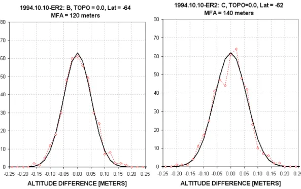
By subtracting the MTP-measured IAC from its counterpart synoptic scale version (the 400-km double boxcar smoother version), it is possible to produce a “mesoscale only” IAC. This IAC is free of the systematic errors that would exist if a synoptic scale IAC were used that had been produced from the satellite and RAOB-based analyzed data. It is a simple procedure to characterize the fluctuations of any flight segment of

25

“mesoscale only” isentrope altitude for a specific isentrope by converting the values to a histogram and measuring the histogram’s full-width at half-maximum, FHWM. This was done using a spreadsheet, where fitting the histogram with a Gaussian function was done manually. In almost every case the Gaussian function is a good fit to the observed

ACPD

Full Screen / Esc

Printer-friendly Version Interactive Discussion histogram. Figure 3 is a typical histogram plot that illustrates these differences and the

proper fit of Gaussian representations used to estimate MFA.

4 Model for mesoscale fluctuation amplitude dependencies

MFA was determined from Gaussian fits to mesoscale minus synoptic scale isentrope altitudes for 81 flight segments of 22 ER-2 flights in the Southern Hemisphere. Each

5

MFA value was entered into a spreadsheet with latitude and date. A season parameter called “Winterness” was calculated for each entry that varied in a sinusoidal manner from 0.0 on 15 July to 1.0 on 15 January (described in detail in the companion article). An MFA was categorized as belonging to “summer” if Winterness <0.4, and it was

categorized as “winter” when Winterness>0.6. Winterness values between 0.4 and

10

0.6 were categorized as “spring.”

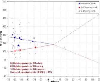
Figure 4 shows the individual MFA measurements plotted versus latitude, with dif-ferent symbols for winter and summer seasons. This figure exhibits a much greater seasonal overlap of individual MFA measurements for all latitude regions compared with measurements for NH (Fig. 1). To aid in illustrating the presence of a seasonal

15

effect the MFA entries for a season were arranged by latitude in groups of ∼6 and a median combine of MFA was calculated. The median combine MFA values show a clear pattern of greater MFA in winter compared with summer. There is also weak evi-dence for an increasing seasonal difference with latitude. Both correlations are present in the NH MFA measurements (Fig. 1).

20

The straight line fits to the summer and winter MFA values in the SH data (Fig. 4) are described by the following equations:

MFA winter [meters] = 116 − 0.27 × Latitude [deg] (1)

MFA summer [meters] = 116 + 0.26 × Latitude [deg] (2)

The dependence on latitude of SH summer and SH winter MFA are approximately

25

ACPD

Full Screen / Esc

Printer-friendly Version Interactive Discussion difference between the SH and NH measurements is that the latitude dependence for

the SH is 27±8% of the NH latitude dependence.

A multiple regression model was created that incorporates latitude and the seasonal parameter as independent variables. The dependent variable was MFA corrected for altitude. Since the range of altitudes was small an altitude correction exponent could

5

not be solved for, so the correction equation found from NH data was used for correcting the SH MFA:

MFA corrected = MFA × (P[hPa]/58.85)−0.40 ₍₃₎

whereP is air pressure at flight altitude.

The range of altitude corrections was 17% (maximum minus minimum correction).

10

The uncertainty of this correction is considered small compared with the correction, and it is especially small compared with the uncertainty of individual MFA measurements.

The plot of measured versus model MFA in the SH is shown in Fig. 5. The model line in this figure is described by the following equation:

SH MFA [meters] = 114 −0.42 × Latitude [deg] +0.84 × Winterness × Latitude [deg]

±0.17 ±0.22

(4)

15

The companion article concluded with a similar equation except that the coefficients are different:

NH MFA [meters] = 112 −1.21 × Latitude [deg] +2.20 × Winterness × Latitude [deg]

±0.27 ±0.20 (5)

This version of the NH model corresponds to flight over ocean (“topography parameter” = zero) and at ER-2 altitudes (19.4 km). It is apparent that the SH coefficients are

20

significantly smaller than the corresponding NH coefficients. The ratio of the latitude coefficients is 0.35±0.15. The ratio of the “Winterness × Latitude” terms is 0.38±0.09. It is significant that the signs of corresponding terms are the same, and the constant terms (114 and 112) are essentially the same.

ACPD

Full Screen / Esc

Printer-friendly Version Interactive Discussion

5 Conclusion

“Mesoscale temperature fluctuations” can be inferred from the amplitude of mesoscale “wrinkles” of isentrope altitude cross-sections. The mesoscale fluctuation amplitudes (MFA) of these wrinkles is smaller in the Southern Hemisphere than the Northern Hemi-sphere. When allowance is made for the dependence of MFA upon latitude, season,

5

topography and altitude, it is found that the ratio of SH to NH MFA is 37±11%.

Acknowledgements. The research described in this publication was carried out by the Jet

Propulsion Laboratory, California Institute of Technology, under a contract with the National Aeronautics and Space Administration. Specific acknowledgement is made for the contribu-tions of R. Denning for his instrument construction and support throughout all field uses of the

10

Microwave Temperature Profiler. I thank M. J. Mahoney for assuming all MTP responsibilities after my retirement and for his encouragement to bring this work to publication.

References

Gary, B. L.: Mesoscale temperature fluctuations in the stratosphere, Atmos. Chem. Phys., 6, 4577–4589, 2006,

15

ACPD

Full Screen / Esc

Printer-friendly Version Interactive Discussion Fig. 1. Northern Hemisphere measurements of MFA versus latitude for winter (blue asterisks)

ACPD

Full Screen / Esc

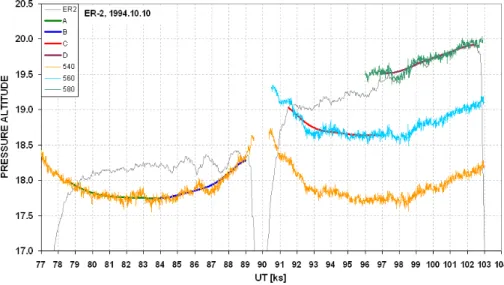
Printer-friendly Version Interactive Discussion Fig. 2. Isentrope altitude cross-section for an ER-2 flight based in Christchurch, NZ. Altitudes

for 540, 560 and 580 K isentrope surfaces are also represented by synoptic scale versions (smooth thick traces, flight segments A, B, C and D) using a 400 km double boxcar averaging procedure. The ER-2 flight altitude (light gray trace) shows a brief descent to ∼15 km (made for in situ air sampling) at the south end of the flight (at ∼90 ks).

ACPD

Full Screen / Esc

Printer-friendly Version Interactive Discussion Fig. 3. Histograms of differences between mesoscale altitudes and synoptic scale altitudes for

ACPD

Full Screen / Esc

Printer-friendly Version Interactive Discussion Fig. 4. Southern Hemisphere measurements of MFA during winter (blue), spring (gray) and

summer (red). The large solid-color diamonds are a median combine of 6 individual MFA measurements (grouped by latitude). The dashed lines for NH latitudes correspond to the model fits to NH measurements as described in the companion article. All MFA have been adjusted to a 19.4 km reference altitude using an altitude exponent of −0.40 (discussed in the text).

ACPD

Full Screen / Esc

Printer-friendly Version Interactive Discussion Fig. 5. Measured MFA (for SH) versus MFA predicted by model that includes a dependence on

latitude, season and altitude. The blue squares are median combined versions of 7 individual flight segment measurements (using predicted MFA for grouping). R-squared = 0.64 for the median combined values.