Observation of strongly heterogeneous dynamics at the depinning transition in a colloidal glass

the depinning transition in a colloidal glass

Nesrin S¸enbil,1, ∗ _{Markus Gruber,}2, ∗ _{Chi Zhang,}1 _{Matthias Fuchs,}2 _{and Frank Scheffold}1 1_{Department of Physics, University of Fribourg, CH-1700 Fribourg, Switzerland}

2

Fachbereich Physik, Universit¨at Konstanz, 78457 Konstanz, Germany (Dated: December 6, 2018)

Sample preparation protocol.– We prepare uniform oil-in-water emulsions as described pre-viously [1, 2]. The oil phase consists of PMHS (Poly(methylhydrosiloxane), Sigma-Aldrich cat. no:176206). First, a crude emulsion is prepared using a custom made Couette shear cell, stabilized with SDS (Sodium dodecyl sulfate) and subsequently size segregated by depletion fractionation until the desired size polydispersity of approximately 12% (standard deviation/mean) is reached [3]. The droplet mean diameter of d = 2.01 ± 0.05 µm and the polydispersity were determined by multi-angle dynamic light scatter-ing (LS Spectrometer, LS Instruments, Switzerland). Confocal microscopy of a dye-labeled sample were found in agreement with these results. We replace SDS by the block-copolymer surfactant Pluronic F108 (BASF, Germany) to achieve steric stabilization of the emulsion droplets. For the active microrheology experiments, the solvent and the emulsion droplets are refractive index and buoyancy matched at room temperature T = 22◦C by replacing the aqueous solvent with a mixture of water, DMAC and Formamide, volume ratio 6:4:1 [1]. As shown previously we can control the droplet volume fraction to better than 3 × 10−3when taking the jamming condition at φJ = 0.642 as a reference [1, 2]

(see Figure S1). In the present study we add a small amount of polystyrene particles (PS), volume fraction about 10−4, of the same size to serve as microrheological probes. The PS particles (micromod, Germany, product 01-54-203) have a diameter 2µm and polydispersity 5% (standard deviation/mean, supplier information). The particle are stabilized with a coating of polyethylene glycol (mol. weight 300 g/mol). The refractive index is n ' 1.6, significantly higher than the solvent and the droplets n = 1.40 which provides contrast for the optical tweezer and allows us to apply a force on the particle. The sample is filled in a custom made plastic cell (thickness 200 µm, area 3.1mm2_{), and closed with}

glass cover slip placed under a microscope objective combined with a laser tweezer setup.

We centrifuge the fractionated emulsion at 4◦C and 4000rpm overnight. Lowering the temperature to 4◦C induces a slight density mismatch between the emulsion droplets and the solvent and consequently a solid plug is formed at the bottom of the cuvette. Then, trace amounts of polystyrene probe particles are dispersed into the sample. By choosing a sufficiently high starting

concentration for the emulsion we make sure that the PS particles do not sediment or cream and remain dilute throughout the sample, even though they are not perfectly buoyancy matched with the bath (The density of the solvent and the oil is 1.006 g/ml at 22◦C while the density of the polystyrene particles is 1.03 g/ml). Samples with different compositions are obtained by dilution with the solvent phase.

Determination of the unjamming transition by dynamic light scattering.– The accuracy of directly measuring droplet fractions by drying and weighing is limited, as discussed e.g. in [4]. Therefore we chose dynamic light scattering (DLS) as a sensitive tool to determine the unjamming point of our emulsion precisely which we can then use as a reference. The sample at

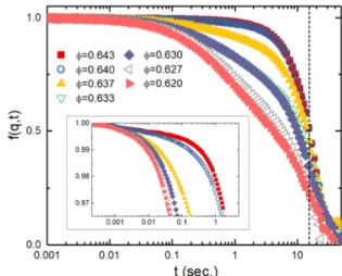
FIG. S1. Intermediate scattering function for different emul-sion concentrations φ. Measurements are taken at an angle of 90◦which corresponds to qd = 37.8 for the incident laser light of wavelength λ = 660nm. Inset: Enlarged view of the same data for f (q, t) close to one.

this composition is then set to φJ = 0.642 as predicted

by computer simulations for hard-sphere or nearly hard spheres systems with 12% polydispersity [1, 5]. Dilution of the stock emulsion can be done very precisely since we can measure the weight and volume of the added solvent accurately and we know that the density of the solvent and the oil are the same. To determine the unjamming point we dilute an as-prepared jammed stock emulsion in small steps and record the normalized intensity-intensity autocorrelation function g2(t) − 1 using a commercial

0.001 rpm [6]. In the jammed state, the elastic modulus of the sample is rather high and droplets are in contact f (q, t)sample ' 1. The rotation, however, induces a

terminal decay of f (q, t) at about t = 10 − 20 sec as can be seen clearly in Figure S1. Upon dilution of the sample, the free volume per particle becomes finite and we observe an additional decay, associated with the local motion of the droplets (also known as the β-relaxation). Figure S1 clearly shows the sensitivity of our experiment to this effect. Initially the curves are nearly flat f (q, t) ' 1 indicating a highly elastic solid which is followed by the decay due to the rotation of the cuvette. At some point we observe first deviations (inset Figure S1). Further decreasing the concentration by only 3 × 10−3 the differences become dramatic. This shows that our DLS-experiments are very sensitive to the unjamming transition. DLS allows us to determine the jamming/unjamming transition with an accuracy better than ∆φ ∼ 3 × 10−3.

Fitting of time and length scales.– To compare experimental results and MCT predictions, we need to find the proper packing-fractions, time- and lengthscales. The corresponding packing-fraction is not fitted but calculated by adjusting the glass transition point via φM CT/0.516 = φexp/0.59. The lengthscale in the system

is determined by the bath particle diameter d. The MCT timescale ¯t is set by the short time diffusion coefficient via ¯t = d2/D0, which coincides with the bare diffusion

coefficient in dilute samples. For dense suspensions, short time diffusion is slower due to interactions (steric and hydrodynamic) and therefore needs to be measured or fitted. Since the MCT glass transition occurs at lower packing fractions, the localization length in the glass is larger than in the experiment. Therefore, we also allow for a fitting of the length-scale ¯d, as has been done in earlier comparisons [7]. We do a least squares fit in the log-log-representation to determine the time-scale and the length-scale for each packing fraction individually. Experimental data and fits are shown in Fig. S2. The fit-parameters can be found in Table I. These length- and time-scales are then used for the following comparison.

Constant force calibration.– While a conventional optical single-beam gradient force trap is characterized by a roughly linear force-distance relation, in our exper-iments, we realize an x−position independent constant force by using a time shared line trap configuration

(Fig-FIG. S2. Thermally driven motion (F ≡ 0). 2D mean square displacement (MSD) h∆x2_{(t) + ∆y}2_{(t)i of the}

emul-sion droplets at different packing fractions φ (filled circles). Solid lines are calculated MSD obtained from MCT. For φ ≥ φg ' 0.59 the sample is dynamically arrested. Right

col-umn: Circles show corresponding examples for the displace-ments (∆x(t), ∆y(t)) tracked in a 2D-plane for same φ over a duration of 1200 seconds. The diameter of the circles is d=2µm.

TABLE I. Corresponding parameters between experiments and MCT φexp φMCT ¯t (s) D0= d2/¯t (µm2/s) d/d¯ 0.535 0.47 167 0.0237 0.795 0.545 0.48 1090 0.00366 0.965 0.575 0.50 2310 0.00173 1.21 0.595 0.52 3500 0.00114 1.20 0.601 0.525 2790 0.00144 1.12

ure S3). We use a high power infrared laser λ = 1064nm as a light source (IPG Photonics, USA, 10W). To be able to compare different experiments we measure the laser power Pl(mW) after the AOM (before the lens 1)

using a set of attenuators and a power meter (Thorlabs, USA). The actual laser power incident on the sample is about 30 × higher, typically of the order of 0.1 − 1 Watt distributed over a line of length x0= 40µm.. The

laser beam is expanded to fill the back aperture of a microscope 60X microscope objective. We can control the incident angle, perpendicular to the direction of propagation, using two fast acousto optical modulators (AOM’s). The angular displacement allows us to control the x, y position in a the focal plane of the objective, which is adjusted to be parallel to the glass interface of the sample cell layer. In the present experiment we only displace the beam along the x− axis to create a line trap. The voltage sequence was designed such that the OT is distributed along a line (e.g. x ∈ [0, x0]) in a random

manner. Moreover, the density probability function ρ of the OT position is set to increase linearly ρ(x) = kx with

FIG. S3. Schematic of the optical tweezer and imaging setup. IR-laser: Infrared laser λ=1064nm with up to 10Watt output power. Two crossed acousto optical modulators (AOM’s). L1 and L2: Lenses with focal length L1 = 100mm and

L2 = 250mm. IR reflective dichroic mirror, inverted Nikon

TS100 microscope body with a 60X/1.40 Nikon objective em-ployed to form a tightly focused spot inside the sample. The AOM’s and the back aperture of the objective are located in conjugate planes. The z−position can be adjusted with the TS100 body. On top of the objective a glass cell con-taining the sample is placed on a x − y translation stage. White light illumination from the top and image recorded of the sample with a digital camera through a dichroic mir-ror. The control of the AOM and the data acquisition is per-formed with two National Instruments controller cards (NI-BNC-21110 and NI-PCI-6229) and a personal computer (PC).

ρ(0) = 0 and k =constant. The force (along the line) acting on the probe located at x from the OT positioned at x + ξ can be denoted as f (ξ), where ξ ∈ [−ξ0, ξ0].

Here ±ξ0 denotes the finite range over which the OT

can influence the probe and ξ is the relative distance between the OT and the probe. For positions far from both ends of the trap, i.e. x ∈ [ξ0, x0− ξ0], the total

force applied on the probe can be written as

F (x) = Z ξ0

−ξ0

ρ(x + ξ)f (ξ)dξ. (S1)

Since ρ(x) = kx, equation (S1) can be rewritten as

F (x) = Z ξ0 −ξ0 ρ(x)f (ξ)dξ + Z ξ0 −ξ0 ρ(ξ)f (ξ)dξ. (S2)

Since f (ξ) = −f (−ξ), the first term of equation (S2) is zero, meaning that F (x) is independent of x. Thus, the total force is constant F (x) ≡ F , within the range of x ∈ [ξ0, x0− ξ0]. Since roughly ξ0 ' 2λ ' 2µm [8]

for objectives with numerical aperture ' 1.4 and in our case x0 ' 40 µm, we therefore obtain a constant force

over a large x-range. We note that all components of the forces scale with the laser power selected. While Fy and

Fz point towards ∆y, ∆z = 0, Fx ≡ F is constant and

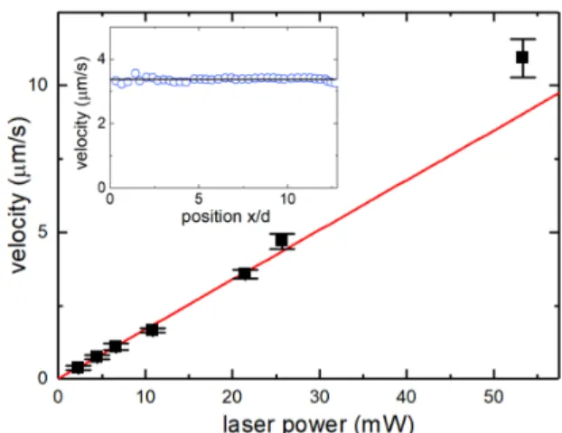
FIG. S4. Velocity v of a probe particle in the bulk of a simple liquid with the same refractive index as the emul-sion sample. The probe particle velocity, and thus the ap-plied force, increases proportionally with the incident laser power setting Pl. Inset: For a given laser power the velocity

(shown: v = 3.37 ± 0.06µm/s, Pl=21.5 mW) is constant over

an x− range of more than 12 particle diameters d. In the stationary state the applied force is balanced by the stokes drag FStokes = ζv. Using the bulk viscosity of the solvent

η ' 4 mPa s to calculate the Stokes drag ζ = 3πηd we find F ' 12.8 × PlfN/mW.

points in positive x-direction.

To verify the successful implementation of the constant force line trap we measure the velocity of the PS probe particle in a pure solvent mixture of water and DMAC (volume ratio 1:1.15) with a viscosity η ' 4 mPa s and a refractive index matched to the index of the emulsion droplets [9]. Figure S4 a) shows that the velocity is in-deed constant, within better than 2%, over a range of more than 12 particle diameters in x−direction corre-sponding to more than 25µm. Moreover, as shown in Figure S4, the velocity increases linearly with the power Pl(mW) of the laser. This demonstrates that we can

precisely control the constant force applied to the probe particle. From the velocity measurements we can esti-mate that we are able to apply forces in the range of sev-eral hundreds of femtonewtons. In the emulsion, residual scattering from the droplets might somewhat perturb the line trap. This is discussed in the Section Linear response calibration.

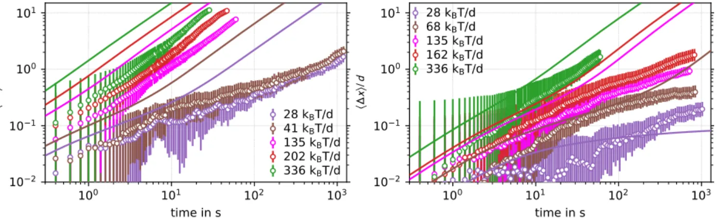
Mean displacements.– The raw mean displacements as obtained by averaging all particle positions at a given time are shown in Fig. S5 in the liquid (φ = 0.535, left panel) and in the glass (φ = 0.601, right panel). Error-bars indicate statistical and systematic uncertainties; see the main text for discussion. The theory curves are ob-tained using the same forces as the experiments and the corresponding MCT packing fraction. In particular, no fitting has been done. We find a stronger localization in the experiment than predicted. We tentatively attribute

10

₁₀

₁₀

₁₀

time in s

10

336 k

T/d

10

₁₀

₁₀

₁₀

time in s

10

FIG. S5. Mean displacements h∆x(t)i in liquid at φ = 0.535 (left), and in the glass φ = 0.601 (right). Error bars indicate the standard deviation of the mean and the systematic uncertainties for the start of the trajectories. Theory curves (solid lines) are obtained for the same force at the corresponding MCT packing fraction. No fitting is done.

a part of this difference to the use of a line-trap with a confining lateral potential. A build-up of bath particles in front of the probe may slow it down compared to when the perpendicular motion can fluctuate freely.

28 kBT/d 68 kBT/d 135 kBT/d 162 kBT/d 336 kBT/d 10-2 10-3 10-4 <∆ x> kB T/Fd 2 t(s) 101 100 ₁₀2 ₁₀3 <∆x2_>/2,Exp

FIG. S6. Rescaled mean displacements in the glass at φ = 0.601; the corresponding plot for the fluid is shown as Fig. 2 in the main text. The raw displacements are divided by the non-dimensionalized force and compared to the quiescent mean squared displacement h∆x2ieq(circles). The shaded area

in-dicates the uncertainty which arises from the difficulties in determining the starting position and time. Error bars (sta-tistical uncertainties) are plotted for one value of the force only for clarity (full set is shown in Fig. S5).

Linear response calibration.– In the laser tweezer calibration in a simple liquid it was found that the force F of the laser tweezer is proportional to the actual laser power Pl via F = cPl with c = 6.3 kBT /mW= 12.8

fN/mW, Figure S4. Although there is no reason for this proportionality to break down in the emulsion, there is the possibility of additional losses, e.g. due to scattering and optical abberations, which will reduce the prefac-tor of this proportionality relation. Therefore, we

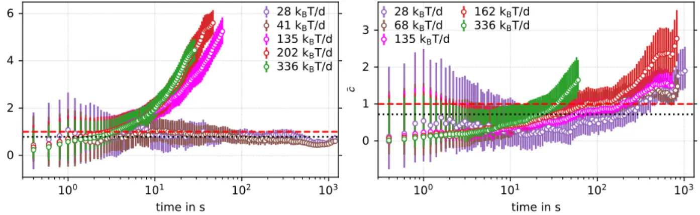
mea-sure this prefactor using a linear response analysis in the emulsion. The linear response relation Eq. (1) relates the mean displacement to the mean squared displace-ment without external force, see Fig. S2. In Fig. 2 of the main text we show this relation for the fluid and in Fig. S6 we show it for the glass. For a more quantitative comparison, we calculate ¯ c(t) = 2hx(t)i h∆x2_(t)i eq kBT F (S3)

for every t and every force available, which is shown in Fig. S7. From Eq. (1) we expect ¯c(t) = 1 in the lin-ear response regime. It can be seen that this relation holds quite well over the full range of times t explored for small forces for φ = 0.535. For the sample in the glass φ = 0.601 this relation is true for times between 50 and 100 seconds. The short times might be off due to the uncertainties about the initial position and starting time. Averaging all data points for forces below 100 kBT /d (for

φ = 0.535) and below 180 kBT /d (for φ = 0.601) leads

to ¯c ≈ 0.75, indicating that the forces are about 25% smaller than in the dilute system.

Theory details.– The MCT approach to microrhe-ology was developed in [10] and the calculation is per-formed using the algorithm described there. The time grid for the integrodifferential equations is uniform with 1024 grid points and an initial time step of ∆t = 10−8. Whenever the end of this grid is reached, the time step is doubled and the results are decimated. The q-space is discretized on a combined logarithmic and uniform grid. The uniform part of the grid has 101 points rang-ing from qd = 0 to qd = 15; in the logarithmic part the stepsize of the uniform grid is halved 10 times. This results in the following grid points: [0,1.5E-4,3E-4,. . . ,0.075,0.15,0.3,0.45,. . . ,15]. For this discretization of

10

₁₀

₁₀

₁₀

time in s

0

2

4

6

28 k

T/d

41 k

T/d

135 k

T/d

202 k

T/d

336 k

T/d

10

₁₀

₁₀

₁₀

time in s

0

1

2

3

28 k

68 k

T/d

T/d

135 k

T/d

162 k

T/d

336 k

T/d

FIG. S7. Linear response factor ¯c (see Eq. (S3) for φ = 0.535 (left) and φ = 0.601 (right). The red dashed line shows the expected value ¯c = 1. The dotted black line shows the value obtained by averaging all data-points for all forces for which linear response holds.

the system, the critical force is Fc= 34.3856869kBT /d.

∗

these authors contributed equally

[1] C. Zhang, C. B. O’Donovan, E. I. Corwin, F. Cardinaux, T. G. Mason, M. E. M¨obius, and F. Scheffold, Physical Review E 91, 032302 (2015).

[2] C. Zhang, N. Gnan, T. G. Mason, E. Zaccarelli, and F. Scheffold, Journal of Statistical Mechanics: Theory and Experiment 2016, 094003 (2016).

[3] T. Mason, A. Krall, H. Gang, J. Bibette, and D. A. Weitz, Encyclopedia of Emulsion Technology 4, 299

(1996).

[4] C. P. Royall, W. C. Poon, and E. R. Weeks, Soft Matter 9, 17 (2013).

[5] K. W. Desmond and E. R. Weeks, Physical Review E 90, 022204 (2014).

[6] J.-Z. Xue, D. Pine, S. Milner, X.-l. Wu, and P. Chaikin, Physical Review A 46, 6550 (1992).

[7] M. Sperl, Physical Review E 71 (2005), 10.1103/Phys-RevE.71.060401.

[8] M. Woerdemann, in Structured Light Fields (Springer, 2012) pp. 5–26.

[9] T. M. Aminabhavi and B. Gopalakrishna, Journal of Chemical and Engineering Data 40, 856 (1995).

[10] M. Gruber, G. C. Abade, A. M. Puertas, and M. Fuchs, Physical Review E 94, 042602 (2016).