HAL Id: hal-01333645
https://hal.inria.fr/hal-01333645
Submitted on 18 Jun 2016
HAL is a multi-disciplinary open access
archive for the deposit and dissemination of
sci-entific research documents, whether they are
pub-lished or not. The documents may come from
teaching and research institutions in France or
L’archive ouverte pluridisciplinaire HAL, est
destinée au dépôt et à la diffusion de documents
scientifiques de niveau recherche, publiés ou non,
émanant des établissements d’enseignement et de
recherche français ou étrangers, des laboratoires
Implementing multifrontal sparse solvers for multicore
architectures with Sequential Task Flow runtime systems
Emmanuel Agullo, Alfredo Buttari, Abdou Guermouche, Florent Lopez
To cite this version:
Emmanuel Agullo, Alfredo Buttari, Abdou Guermouche, Florent Lopez. Implementing multifrontal
sparse solvers for multicore architectures with Sequential Task Flow runtime systems. ACM
Trans-actions on Mathematical Software, Association for Computing Machinery, 2016, �10.1145/2898348�.
�hal-01333645�
Implementing multifrontal sparse solvers for multicore architectures
with Sequential Task Flow runtime systems
Emmanuel Agullo, Inria-LaBRI
Alfredo Buttari, CNRS-IRIT
Abdou Guermouche, Universit´e de Bordeaux
Florent Lopez, UPS-IRIT
To face the advent of multicore processors and the ever increasing complexity of hardware architectures, pro-gramming models based on DAG parallelism regained popularity in the high performance, scientific comput-ing community. Modern runtime systems offer a programmcomput-ing interface that complies with this paradigm and powerful engines for scheduling the tasks into which the application is decomposed. These tools have already proved their effectiveness on a number of dense linear algebra applications. This paper evaluates the usability and effectiveness of runtime systems based on the Sequential Task Flow model for complex ap-plications, namely, sparse matrix multifrontal factorizations which feature extremely irregular workloads, with tasks of different granularities and characteristics and with a variable memory consumption. Most importantly, it shows how this parallel programming model eases the development of complex features that benefit the performance of sparse, direct solvers as well as their memory consumption. We illustrate our discussion with the multifrontal QR factorization running on top of the StarPU runtime system.
Categories and Subject Descriptors: D.1.3 [Programming Techniques]: Concurrent Programming; G.1.3 [Numerical Analysis]: Numerical Linear Algebra; G.4 [Mathematical Software]
General Terms: Algorithms, Performance
Additional Key Words and Phrases: Sparse direct solvers, multicores, runtime systems, communication-avoiding, memory-aware
ACM Reference Format:
Emmanuel Agullo, Alfredo Buttari, Abdou Guermouche and Florent Lopez, 2014. Implementing multifrontal sparse solvers for multicore architectures with Sequential Task Flow runtime systems ACM Trans. Math. Softw. V, N, Article A (January YYYY), 23 pages.
DOI:http://dx.doi.org/10.1145/0000000.0000000 1. INTRODUCTION
The increasing degree of parallelism and complexity of hardware architectures re-quires the High Performance Computing (HPC) community to develop more and more complex software. To achieve high levels of optimization and fully benefit from their potential, not only the related codes are heavily tuned for the considered architecture, but the software is furthermore often designed as a single whole that aims to cope with both the algorithmic and architectural needs. If this approach may indeed lead to extremely high performance, it is at the price of a tremendous development effort and a decreased maintainability.
This work is supported by the Agence Nationale de la Recherche, under grant ANR-13-MONU-0007. This work was performed using HPC resources from GENCI-[CCRT/TGCC/CINES/IDRIS] (Grant 2014-i2014065063)
Permission to make digital or hard copies of part or all of this work for personal or classroom use is granted without fee provided that copies are not made or distributed for profit or commercial advantage and that copies show this notice on the first page or initial screen of a display along with the full citation. Copyrights for components of this work owned by others than ACM must be honored. Abstracting with credit is per-mitted. To copy otherwise, to republish, to post on servers, to redistribute to lists, or to use any component of this work in other works requires prior specific permission and/or a fee. Permissions may be requested from Publications Dept., ACM, Inc., 2 Penn Plaza, Suite 701, New York, NY 10121-0701 USA, fax +1 (212) 869-0481, or [email protected].
c
YYYY ACM 0098-3500/YYYY/01-ARTA $15.00 DOI:http://dx.doi.org/10.1145/0000000.0000000
Alternatively, a modular approach can be employed. First, the numerical algorithm is written at a high level independently of the hardware architecture as a Directed Acyclic Graph (DAG) of tasks where a vertex represents a task and an edge repre-sents a dependency between tasks. A second layer is in charge of the scheduling. This layer decides when and where (which Processing Unit) to execute a task. Based on the scheduling decisions, a runtime engine, in the third layer, retrieves the data neces-sary for the execution of a task (taking care of ensuring the coherency among multiple possible copies), triggers its execution and updates the state of the DAG upon its com-pletion. The border between the scheduling and runtime layers is a bit variable and ultimately depends on the design choices of the runtime system developers. The fourth layer consists of the tasks code optimized for the underlying architectures. In most cases, the bottom three layers need not be written by the application developer. Indeed, it is usually easy to find off the shelf a very competitive, state-of-the-art and generic scheduling algorithm (such as work-stealing [Arora et al. 2001], Minimum Completion Time [Topcuouglu et al. 2002]) that matches the algorithmic needs to efficiently exploit the targeted architecture. Otherwise, if needed, as we do in this study for efficiently handling tasks of small granularity, a new scheduling algorithm may be designed (and shared with the community to be in turn possibly applied to a whole class of algo-rithms). The runtime engine only needs to be extended once for each new architecture. Finally, in many cases, the high-level algorithm can be cast in terms of standard op-erations for which vendors provide optimized codes. In other common cases, available kernels only need to be slightly adapted in order to take into account the specificities of the algorithm; this is, for example, the case of our method where the most com-putationally intensive tasks are minor variants of LAPACK routines (as described in Section 4.3. All in all, with such a modular approach, only the high-level algorithm has to be specifically designed, which ensures a high productivity. The maintainability is also guaranteed since the use of new hardware only requires (in principle) third party effort. Modern tools exist that implement the two middle layers (the scheduler and the runtime engine) and provide a programming model that allows the programmer to conveniently express his workload in the form of a DAG of tasks; we refer to these tools as runtime systems or, simply, runtimes.
The dense linear algebra community has strongly adopted such a modular approach over the past few years [Buttari et al. 2009; Quintana-Ort´ı et al. 2009; Agullo et al. 2009; Bosilca et al. 2013] and delivered production-quality software relying on it. How-ever, beyond this community, only few research efforts have been conducted to handle large scale codes. The main reason is that irregular problems are complex to design with a clear separation of the software layers without inducing performance loss. On the other hand, the runtime system community has strongly progressed, delivering very reliable and effective tools [Augonnet et al. 2011; Bosilca et al. 2012; Badia et al. 2009; Hermann et al. 2010] up to the point that the OpenMP board has included simi-lar features in the latest OpenMP standard 4.0 [2013].
In the past [Buttari 2013], we have assessed the effectiveness of a DAG based par-allelization of the QR factorization of sparse matrices and later on [Agullo et al. 2013] we proposed an approach for implementing this method using a runtime system.
This work extends our previous efforts and other related works in three different ways:
(1) It proposes a parallelization purely based on a Sequential Task Flow (STF) model: our previous work [Agullo et al. 2013] proposed a rather complex strategy for sub-mitting tasks to the runtime system which renders the code difficult to maintain and to update with new features and algorithms; here, instead, we propose an
approach that relies on the simplicity and effectiveness of the STF programming model.
(2) It uses 2D Communication Avoiding algorithms (for the sake of readability we will refer to these techniques as “2D algorithms” from now on) for the QR factorization of frontal matrices: in the very common case where frontal matrices are (strongly) overdetermined, the block-column partitioning used in our previous work repre-sents a major scalability problem. Here we propose a 2D partitioning of frontal matrices into tiles (i.e., blocks) and the use of factorization algorithms by tiles, of-ten referred to as Communication Avoiding algorithms. Note that the use of 2D front factorization algorithms was introduced in the work by Yeralan et al. [Yer-alan et al. 2015] and implemented in the SuiteSparseQR [Davis 2014] package. In Section 4.2 we comment on the differences about our approach and theirs.
(3) It proposes a memory-aware approach for controlling the memory consumption of the parallel multifrontal method, which allows the user to achieve the highest possible performance within a prescribed memory footprint. This technique can be seen as employing a sliding window that sweeps the whole elimination tree and whose size is dynamically adjusted in the course of the factorization in order to accommodate for as many fronts as possible within the imposed memory envelope. These three contributions are deeply related. The approach based on 2D frontal ma-trix factorizations leads to extremely large DAGs with heterogeneous tasks and very complex dependencies; implementing such a complex algorithm in the STF model is conceptually equivalent to writing the corresponding sequential code because paral-lelism is handled by the runtime system. The effectiveness of this approach is sup-ported by a finely detailed analysis based on a novel method which allows for a very accurate profiling of the performance of the resulting code by quantifying separately all the factors that play a role in the scalability and efficiency of a shared-memory code (granularity, locality, overhead, scheduling). This method can be readily extended to the case of distributed-memory parallelism in order to account for other performance critical factors such as the communications. Our analysis shows that the runtime sys-tem can handle very efficiently such complex DAGs and that the relative runtime over-head is only marginally increased by the increased DAGs size and complexity; on the other hand, the experimental results also show that the higher degree of concurrency provided by 2D methods can considerably improve the scalability of a sparse matrix QR factorization. Because of the very dynamic execution model of the resulting code, concerns may arise about the memory consumption; we show that, instead, it is possi-ble to control the memory consumption by simply controlling the flow of tasks in the runtime system. Experimental results demonstrate that, because of the high concur-rency achieved by the 2D parallelization and because of the efficiency of the underly-ing runtime, the very high performance of our code is barely affected even when the parallel code is constrained to run within the same memory footprint as a sequential execution.
It must be noted that the proposed techniques are not tied to the multifrontal QR algorithm and can be readily applied to any sparse matrix factorization method. In fact, their scope can be even larger than sparse factorizations as they may be of interest for other algorithms with complex workloads and irregular data access patterns.
The approach proposed here is related to previous work on the PaStiX solver [La-coste et al. 2014] where the StarPU runtime system is used to implement supernodal Cholesky and LU factorizations for multicore architectures equipped with GPUs. In the proposed solution, however, dependencies among tasks are explicitly declared and therefore the approach does not take full advantage of the Sequential Task Flow pro-gramming model provided by StarPU (see Section 3 for the details). In this work, the
authors also proposed a variant based on the PaRSEC (formerly DAGuE) runtime system (which features a different programming model) and presented a comparison between the two implementations. More recently, an article by Kim et al. [2014] pre-sented a DAG-based approach for sparse LDLT factorizations. In this work OpenMP tasks are used where inter-node dependencies (by node, here, we refer to the elimina-tion tree nodes, as described in Secelimina-tion 2) are implicitly handled through a recursive submission of tasks, whereas intra-node dependencies are essentially handled manu-ally.
The rest of this paper is organized as follows. In sections 2 and 3 we describe the con-text of our work giving a brief description of the multifrontal QR method and of mod-ern runtime systems along with the STF parallel programming model. In Section 4.1 we show how the STF model can be used to implement the block-column paralleliza-tion approach described in our previous work [Buttari 2013] with a very compact and elegant code. In the subsequent Section 4.2 we explain how performance can be im-proved by using communication-avoiding, tiled factorizations for frontal matrices. In Section 4.4 we propose a technique for achieving the multifrontal factorization within a prescribed memory consumption. In Section 5 we provide and analyze experimental results showing the effectiveness of the proposed techniques within the qr mumps code using the StarPU runtime system.
2. THE MULTIFRONTAL QR METHOD AND QR MUMPS
The multifrontal method, introduced by Duff and Reid [1983] as a method for the factorization of sparse, symmetric linear systems, can be adapted to the QR factor-ization of a sparse matrix thanks to the fact that the R factor of a matrix A and the Cholesky factor of the normal equation matrix ATA share the same structure under the hypothesis that the matrix A is Strong Hall. As in the Cholesky case, the mul-tifrontal QR factorization is based on the concept of elimination tree introduced by Schreiber [1982]. This graph, which has a number of nodes that is typically one or-der of magnitude or more smaller than the number of columns in the original matrix, expresses the dependencies among the computational tasks in the factorization: each node i of the tree is associated with ki unknowns of A and represents an elimination step of the factorization. The coefficients of the corresponding ki columns and all the other coefficients affected by their elimination are assembled together into a relatively small dense matrix, called frontal matrix or, simply, front, associated with the tree node. The multifrontal QR factorization consists in a tree traversal in a topological
order (i.e., bottom-up) such that, at each node, two operations are performed. First,
the frontal matrix is assembled by stacking the matrix rows associated with the ki unknowns with uneliminated rows resulting from the processing of child nodes. Sec-ond, the ki unknowns are eliminated through a complete QR factorization of the front. This produces kirows of the global R factor, a number of Householder reflectors that implicitly represent the global Q factor and a contribution block formed by the remaining rows. Those rows will be assembled into the parent front together with the contribution blocks from all the sibling fronts. The main differences with the better known multifrontal Cholesky factorization are:
(1) Frontal matrices are generally rectangular (either over or under-determined) and not square;
(2) Frontal matrices are completely and not partially factorized;
(3) Assemblies are not extend-add operations but simple memory copies, which means that they can be executed in an embarrassingly parallel fashion;
(4) Frontal matrices are not full but have a staircase structure: once a frontal matrix is assembled, its rows are sorted in order of increasing index of the leftmost nonzero.
The number of operations can thus be reduced, as well as the fill-in in the Q matrix, by ignoring the zeroes in the bottom-left part of the frontal matrix.
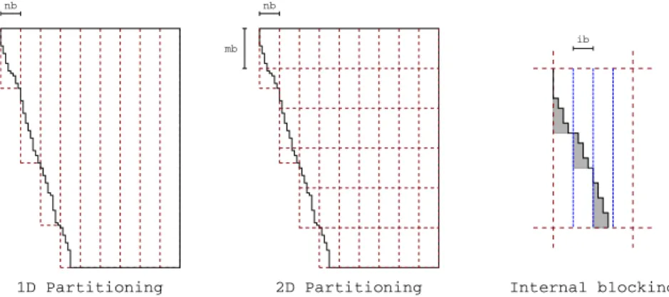
A detailed presentation of the multifrontal QR method, including the optimization techniques described above, can be found in the work by Amestoy et al. [1996]. The classical approach to the parallelization of the multifrontal QR factorization [Amestoy et al. 1996; Davis 2011] consists in exploiting separately two distinct sources of con-currency: tree and node parallelism. The first one stems from the fact that fronts in separate branches are independent and can thus be processed concurrently; the sec-ond one from the fact that, if a front is big enough, multiple processes can be used to assemble and factorize it. The baseline of this work, instead, is the parallelization model proposed in the qr mumps software [Buttari 2013] which is based on the approach presented earlier in related work on dense matrix factorizations [Buttari et al. 2009] and extended to the supernodal Cholesky factorization of sparse matrices [Hogg et al. 2010]. In this approach, frontal matrices are partitioned into block-columns, as shown in Figure 1 (left), which allows for a decomposition of the workload into fine-grained tasks. 1D Partitioning 2D Partitioning nb mb nb ib Internal blocking
Fig. 1. 1D partitioning of a frontal matrix into block-columns (left), 2D partitioning into tiles (middle) and internal block-column or tile blocking (right)
.
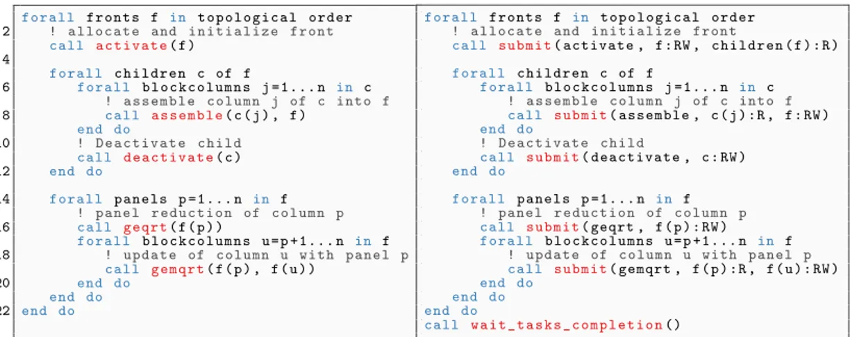
Figure 3 shows on the left-side a simplified sequential pseudocode that achieves the multifrontal QR factorization in the case where a 1D partitioning into block-columns is applied to the frontal matrices. It makes use of five kernels:
(1) activate: this routine allocates and initializes the front data structure;
(2) assemble: for a block-column in the child node c, assembles the corresponding part of the contribution block into f. Note that, in practice, only a subset of the block-columns of f are concerned by this operation which renders most of the assemble tasks independent; the actual parallel implementations presented in our previous works and here, in Section 4, take advantage of this property but for the sake of readability we do not present this level of details in the pseudo-code;
(3) geqrt: computes the QR factorization of a block-column. This is the panel factor-ization in the LAPACK dense QR factorfactor-ization;
(4) gemqrt: applies to a block-column the Householder reflectors computed in a pre-vious geqrt operation. This is the update operations in the LAPACK dense QR factorization;
(5) deactivate: stores the factors aside and frees the memory containing the contri-bution block;
Assuming that each function call in this pseudo-code defines a task, the whole mul-tifrontal factorization can be expressed in the form of a Directed Acyclic Graph (DAG) of tasks. This allows for a seamless exploitation of both tree and node parallelism. Additionally it permits to pipeline the processing of a front with those of its children which provides an additional source of concurrency which we refer to as inter-level parallelism. The benefits of this approach over more traditional techniques have been assessed in our previous work [Buttari 2013].
3. TASK-BASED RUNTIME SYSTEMS AND THE SEQUENTIAL TASK FLOW MODEL
Whereas task-based runtime systems were mainly research tools in the past years, their recent progress makes them now solid candidates for designing advanced sci-entific software as they provide programming paradigms that allow the programmer to express concurrency in a simple yet effective way and relieve him from the bur-den of dealing with low-level architectural details. However, no consensus has still been reached on a specific paradigm. For example, Parametrized Task Graph ap-proaches [Bosilca et al. 2012; Budimli´c et al. 2010; Cosnard and Jeannot 2001] con-sist of explicitly describing tasks (vertices of the DAG) and their mutual dependencies (edges) by informing the runtime system with a set of dependency rules. In such a way, the DAG is never explicitly built but can be progressively unrolled and traversed in a very effective and flexible way. This approach can achieve a great scalability on a very large number of processors but explicitly expressing the dependencies may be a hard task, especially when designing complex schemes.
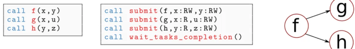
On the other hand, the STF model simply consists of submitting a sequence of tasks through a non blocking function call that delegates the execution of the task to the runtime system. Upon submission, the runtime system adds the task to the current DAG along with its dependencies which are automatically computed through data de-pendency analysis [Allen and Kennedy 2002]. The actual execution of the task is then postponed to the moment when its dependencies are satisfied. This paradigm is also sometimes referred to as Superscalar since it mimics the functioning of superscalar processors where instructions are issued sequentially from a single stream but can actually be executed in a different order and, possibly, in parallel depending on their mutual dependencies. Figure 2 shows a dummy sequential algorithm and its
corre-c a l l f( x , y ) c a l l g( x , u ) c a l l h( y , z ) c a l l s u b m i t( f , x : RW , y : RW ) c a l l s u b m i t( g , x : R , u : RW ) c a l l s u b m i t( h , y : R , z : RW ) c a l l w a i t _ t a s k s _ c o m p l e t i o n()
f
g
h
Fig. 2. Pseudo-code for a dummy sequential algorithm (left), corresponding STF version (center) and subse-quent DAG (right).
sponding STF version. Instead of making three function calls (f, g, h), the equivalent STF submits the three corresponding tasks. The data onto which these functions oper-ate as well as their access mode (Read, Write or Read/Write) are also specified. Because task g accesses data x after task f has accessed it in Write mode, the runtime infers a dependency between tasks f and g. Similarly a dependency is inferred between tasks f and h due to data y. Figure 2 (right) shows the DAG corresponding to this STF dummy code. In the STF model, one thread is in charge of submitting the tasks; we refer to this thread as the master thread. The execution of tasks is instead achieved by worker threads. The function called at the end of the STF pseudo-code is simply a barrier that
prevents the master thread from continuing until all of the submitted tasks are exe-cuted. Note that, in principle, the master thread can also act as a worker; whether this is possible or not depends on the design choices of the runtime system developers. This is not the case in our experimental setting of Section 5.
Many runtime systems [Badia et al. 2009; Kurzak and Dongarra 2009; Augonnet et al. 2011] support this paradigm and a complete review of them is out of the scope of this paper. The OpenMP 4.0 standard, for example, supports the STF model through the task construct with the recently introduced depend clause. Although this OpenMP feature is already available on some compilers (gcc and gfortran, for instance) we chose to rely on StarPU as it provides a very wide set of features that allows, most importantly, for a better control of the tasks scheduling policy and because it supports accelerators and distributed memory parallelism which will be addressed in future work.
4. STF PARALLEL MULTIFRONTAL QR 4.1. 1D, block-column parallelization
As described in Section 3, the STF model is such that the parallelization of a code can be achieved by simply replacing each function call in the sequential code with the sub-mission of a task that achieves the actual execution of that function on a specific data set. Figure 3 (right) shows this transition for the sequential pseudo-code presented in Section 2. The dependencies among the tasks are automatically inferred by the run-time system based on the order of submission and their data access mode; specifically: — the activation of a node f depends on the activation of its children;
— all the other tasks related to a node f depend on the node activation;
— the assembly of a block-column j of a front c into its parent f depends on all the geqrt and gemqrt tasks on c(j) and on the activation of f;
— the geqrt task on a block-column p depends on all the assembly and all the previous update tasks concerning p;
— the gemqrt task on a block-column u with respect to geqrt p depends on all the assembly and all the previous gemqrt tasks concerning u and the related geqrt task on block-column p;
— the deactivation on a front c can only be executed once all the related geqrt, gemqrt and assemble tasks are completed.
As in our previous example of Figure 2, the STF code is concluded with a barrier. This, however, can be removed in order to pipeline the factorization and the solve phase (i.e., the phase where the computed factors are used to solve the linear system) and therefore achieve better performance, assuming the latter is also implemented ac-cording to the STF model. Another possible scenario is where multiple factorizations have to be executed in which case removing the barrier allows for pipelining the suc-cessive operations and thus exploit an additional source of concurrency.
4.2. 2D, communication-avoiding parallelization by tiles
The parallel factorization algorithm presented in the previous section as well as in our previous work [Agullo et al. 2013; Buttari 2013] is based on a 1D partitioning of frontal matrices into block-columns. In this case the node parallelism is achieved because all the updates related to a panel can be executed concurrently and because panel operations can be executed at the same time as updates related to previous panels (this technique is well known under the name of lookahead). It is clear that when frontal matrices are strongly overdetermined (i.e., they have many more rows than columns, which is the most common case in the multifrontal QR method) this
f o r a l l f r o n t s f in t o p o l o g i c a l o r d e r 2 ! a l l o c a t e and i n i t i a l i z e f r o n t c a l l a c t i v a t e( f ) 4 f o r a l l c h i l d r e n c of f 6 f o r a l l b l o c k c o l u m n s j = 1 . . . n in c ! a s s e m b l e c o l u m n j of c i n t o f 8 c a l l a s s e m b l e( c ( j ) , f ) end do 10 ! D e a c t i v a t e c h i l d c a l l d e a c t i v a t e( c ) 12 end do 14 f o r a l l p a n e l s p = 1 . . . n in f ! p a n e l r e d u c t i o n of c o l u m n p 16 c a l l g e q r t( f ( p ) ) f o r a l l b l o c k c o l u m n s u = p + 1 . . . n in f 18 ! u p d a t e of c o l u m n u w i t h p a n e l p c a l l g e m q r t( f ( p ) , f ( u ) ) 20 end do end do 22 end do f o r a l l f r o n t s f in t o p o l o g i c a l o r d e r ! a l l o c a t e and i n i t i a l i z e f r o n t c a l l s u b m i t( a c t i v a t e , f : RW , c h i l d r e n ( f ) : R ) f o r a l l c h i l d r e n c of f f o r a l l b l o c k c o l u m n s j = 1 . . . n in c ! a s s e m b l e c o l u m n j of c i n t o f c a l l s u b m i t( a s s e m b l e , c ( j ) : R , f : RW ) end do ! D e a c t i v a t e c h i l d c a l l s u b m i t( d e a c t i v a t e , c : RW ) end do f o r a l l p a n e l s p = 1 . . . n in f ! p a n e l r e d u c t i o n of c o l u m n p c a l l s u b m i t( geqrt , f ( p ) : RW ) f o r a l l b l o c k c o l u m n s u = p + 1 . . . n in f ! u p d a t e of c o l u m n u w i t h p a n e l p c a l l s u b m i t( gemqrt , f ( p ) : R , f ( u ) : RW ) end do end do end do c a l l w a i t _ t a s k s _ c o m p l e t i o n()
Fig. 3. Pseudo-code for the sequential (left) and STF-parallel (right) multifrontal QR factorization with 1D partitioned frontal matrices
approach does not provide much concurrency. In the multifrontal method this problem is mitigated by the fact that multiple frontal matrices are factorized at the same time. However, considering that in the multifrontal factorization most of the computational weight is related to the topmost nodes where tree parallelism is scarce, a 1D front factorization approach can still seriously limit the scalability.
The node parallelism can be improved by employing 2D dense factorization algo-rithms. Such methods, which have recently received a considerable attention [Don-garra et al. 2013; Demmel et al. 2012; Agullo et al. 2011; Bouwmeester et al. 2011], are based on a 2D decomposition of matrices into tiles (or blocks) of size mb x nb as shown in Figure 1 (middle); this permits to break down the panel factorization and the related updates into smaller tasks which leads to a three-fold advantage:
(1) the panel factorization and the related updates can be parallelized;
(2) the updates related to a panel stage can be started before the panel is entirely reduced;
(3) subsequent panel stages can be started before the panel is entirely reduced. In these 2D algorithms, the topmost panel tile (the one lying on the diagonal) is used to annihilate the others; this can be achieved in different ways. For example, the top-most tile can be first reduced into a triangular tile with a general geqrt LAPACK QR factorization which can then be used to annihilate the other tiles, one after the other, with tpqrt LAPACK QR factorizations, where t and p stand for triangular and pen-tagonal, respectively. The panel factorization is thus achieved through a flat reduction tree as shown in Figure 5 (left). This approach provides only a moderate additional concurrency with respect to the 1D approach because the tasks within a panel stage cannot be executed concurrently; it allows, however, for a better pipelining of the tasks (points 2 and 3 above). Another possible approach consists in first reducing all the tiles in the panel into triangular tiles using geqrt operations; this first stage is embarrass-ingly parallel. Then, through a binary reduction tree, all the triangular tiles except the topmost one are annihilated using tpqrt operations, as shown in Figure 5 (mid-dle). This second method provides better concurrency but results in a higher number of tasks, some of which are of very small granularity. Also, in this case a worse pipelin-ing of successive panel stages is obtained [Dongarra et al. 2013]. In practice a hybrid approach can be used where the panel is split into subsets of size bh: each subset is
re-1 do k =1 , n
! for all the block - c o l u m n s in the f r o n t
3 do i = k , m , bh c a l l s u b m i t( geqrt , f ( k , i ) : RW ) 5 do j = k +1 , n c a l l s u b m i t( gemqrt , f ( k , i ) : R , f ( i , j ) : RW ) 7 end do ! intra - s u b d o m a i n flat - t r e e r e d u c t i o n 9 do l = i +1 , min ( i + bh -1 , s t a i r ( k ) ) c a l l s u b m i t( tpqrt , f ( i , k ) : RW , f ( l , k ) : RW ) 11 do j = k +1 , n c a l l s u b m i t( tpmqrt , f ( l , k ) : R , f ( i , j ) : RW , f ( l , j ) : RW ) 13 end do end do 15 end do do w h i l e ( bh . le . s t a i r ( k ) - k +1) 17 ! inter - s u b d o m a i n s binary - t r e e r e d u c t i o n do i = k , s t a i r ( k ) - bh , 2* bh 19 l = i + bh if( l . le . s t a i r ( k ) ) t h e n 21 c a l l s u b m i t( tpqrt , f ( i , k ) : RW , f ( l , k ) : RW ) do j = k +1 , n 23 c a l l s u b m i t( tpmqrt , f ( l , k ) : R , f ( i , j ) : RW , f ( l , j ) : RW ) end do 25 end if end do 27 bh = bh *2 end do 29 end do
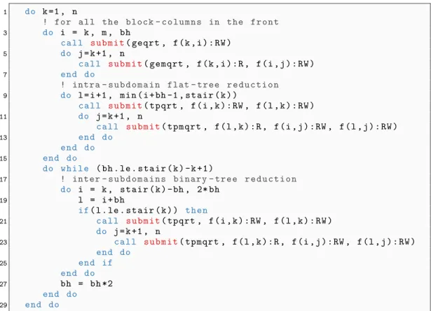
Fig. 4. Pseudo-code showing the implementation of the 2D front factorization. For the sake of readability, this pseudo-code does not handle the case of rectangular tiles. The stair array represents the staircase structure of the front and is such that stair(j) is the row-index of the last tile in block-column j.
duced into a triangular tile using a flat reduction tree and then, the remaining tiles are reduced using a binary tree. This is the technique used in the PLASMA library [Agullo et al. 2009] and illustrated in Figure 5 (right) for the case of bh= 2. Other reduction trees can also be employed; we refer the reader to the work by Dongarra et al. [2013] for an excellent survey of such techniques.
Fig. 5. Possible panel reduction trees for the 2D front factorization. On the (left), the case of a flat tree, i.e., with bh= ∞. In the (middle), the case of a binary tree, i.e., with (bh= 1). On the (right) the case of an hybrid tree with bh= 2.
We integrated the flat/binary hybrid approach described above in our multifrontal STF parallel code. Lines 14-21 in Figure 3 were replaced by the pseudo-code in Figure 4 which implements the described 2D factorization algorithm; note that this code ignores the tiles that lie entirely below the staircase structure of the front represented by the stair array.
As for the assembly operations, they have also been parallelized according to the 2D frontal matrix blocking: lines 6-8 were replaced with a double, nested loop to span all the tiles lying on the contribution block: each assembly operation reads one tile of a node c and assembles its coefficients into a subset of the tiles of its parent f. As a consequence, some tiles of a front can be fully assembled and ready to be processed before others and before the child nodes are completely factorized. This finer granular-ity (with respect to the 1D approach presented in the previous section) leads to more concurrency since a better pipelining between a front and its children is now enabled. In our implementation tiles do not have to be square but can be rectangular with more rows than columns. This is only a minor detail from an algorithmic point of view but, as far as we know, it has never been discussed in the literature and, as described in Section 5, provides considerable performance benefits for our case.
This parallelization leads to very large DAGs with tasks that are very heteroge-neous, both in nature and granularity; moreover, not only intra-fronts task dependen-cies are more complex because of the 2D front factorization, but also inter-fronts task dependencies due to the parallelization of the assembly operations. The use of an STF-based runtime system relieves the developer from the burden of explicitly representing the DAG and achieving the execution of the included tasks on a parallel machine.
As mentioned in Section 1, the use of 2D front factorization algorithms in the multi-frontal QR factorization was already presented in the work by Yeralan et al. [Yeralan et al. 2015] to accelerate the execution on systems equipped with GPU devices. This work relies on a semi static scheduling where lists of ready tasks are produced in suc-cessive steps and offloaded to the GPU. Moreover, the approach proposed therein is not capable of using inter-level parallelism. In our approach, instead, the expressiveness of the STF programming model allows for implementing the 2D front factorization methods as well as the inter-level parallelism in a relatively easy way and therefore achieve a much greater performance also because of a completely dynamic scheduling of tasks, despite the complexity of the resulting DAG. It must also be noted that in the work by Yeralan et al., the scheduling mechanism and the tracking of dependen-cies heavily rely on the knowledge of the algorithm and thus any modification of the front factorization algorithm requires the scheduler to be modified accordingly. In our approach, instead, the expression of the algorithm is completely decoupled from the task dependencies detection and tracking as well as from the scheduling of tasks; this results in a much greater flexibility and ultimately allows for easily improving and modifying the algorithm as well as the scheduling policy.
4.3. Common optimizations
Block storage. Although the partitioning of fronts, either 1D or 2D, may be logical, it is beneficial to store block-columns or tiles in separate arrays as this allows for memory savings because of the staircase structure; this is shown, for example, on block-column 1 in Figure 1 (left) or tile (4,2) in Figure 1 (middle). This feature was not implemented in our previous work [Buttari 2013; Agullo et al. 2013]. In the case of 2D algorithms, this block storage has the further advantage of reducing the stride of accesses to data and, thus, improve the efficiency of linear algebra kernels, as discussed in [Buttari et al. 2009].
Linear algebra kernels. In principle the above parallel algorithms (either 1D or 2D) could be implemented using the standard geqrt, gemqrt, tpqrt and tpmqrt LAPACK routines. This, however, would imply a (considerable) amount of extra-flops because these routines cannot benefit from the fact that, due to the fronts staircase structure, some block-columns (for example 1-4 in Figure 1 (left)) or tiles (for example (1,1) or (3,2) in Figure 1 (middle)) are (mostly) populated with zero coefficients. In this case, the amount of extra-flops depends on the choice of the nb parameter. The above-mentioned LAPACK routines use an internal blocking of size ib in order to reduce the amount of extra flops imposed by the 2D factorization algorithm as explained in [Buttari et al. 2009]. We modified these routines in such a way that the internal blocking is also used to reduce the flop count by skipping most of the operations related to the zeros in the bottom-left part of the tiles lying on the staircase. This is illustrated in Figure 1 (right) where the amount of extra flops is proportional to the gray-shaded area. In such a way, the value of the nb parameter can be chosen only depending on the desired granularity of tasks, without worrying about the flop count.
Tree pruning. The number of nodes in the elimination tree is commonly much larger than the number of working threads. It is, thus, unnecessary to partition every front of the tree and factorize it using a parallel algorithm. For this reason we employ a technique similar to that proposed by Geist and Ng [1989] that we describe in our previous work [Buttari 2013] under the name of “logical tree pruning”. Through this technique, we identify a layer in the elimination tree such that each subtree rooted at this layer is treated in a single task with a purely sequential code. This has a twofold advantage. First it reduces the number of generated tasks and, therefore, the runtime system overhead. Second, it improves the efficiency of operations on those parts of the elimination tree that are mostly populated with small size fronts and, thus, less performance effective. We refer the reader to our previous work [Buttari 2013] and to the original paper by Geist and Ng [1989] for further details on how this level is computed.
For the sake of readability, we did not include the pseudo-code for submitting these subtree tasks in Figures 3 and 4.
4.4. Memory-aware Sequential Task Flow
The memory needed to achieve the multifrontal factorization (QR as well as LU or other types) is not statically allocated at once before the factorization begins but it is allocated and deallocated as the frontal matrices are activated and deactivated, as de-scribed in Section 2. Specifically, each activation task allocates all the memory needed to process a front; this memory can be split into two parts:
(1) a persistent memory: once the frontal matrix is factorized, this part contains the factors coefficients and, therefore, once allocated it is never freed, unless in an out-of-core execution (where factors are written on disk)1;
(2) a temporary memory: this part contains the contribution block and it is freed by the deactivate task once the coefficients it contains have been assembled into the parent front.
As a result, the memory footprint of the multifrontal method in a sequential exe-cution varies greatly throughout the factorization. Starting at zero, it grows fast at the beginning as the first fronts are activated, it then goes up and down as fronts are activated and deactivated until it reaches a maximum value (we refer to this value as 1In some other cases the factors can also be discarded like, for example, when the factorization is done for computing the determinant of the matrix.
the sequential peak) and eventually goes down towards the end of the factorization to the point where the only thing left in memory is the factors. The memory consumption varies depending on the particular topological order followed for traversing the elim-ination tree and techniques exist to determine the memory minimizing traversal for sequential executions [Guermouche et al. 2003].
It has to be noted that parallelism normally increases the memory consumption of the multifrontal method simply because, in order to feed the working processes, more work has to be generated and thus more fronts have to be activated concurrently. The memory consumption of the STF parallel code discussed so far can be considerably higher than the sequential peak (up to 3 times or more). This is due to the fact that the runtime system tries to execute tasks as soon as they are available and to the fact that activation tasks are extremely fast and only depend upon each other; as a result, all the fronts in the elimination tree are almost instantly allocated at the beginning of the factorization. This behavior, moreover, is totally unpredictable because of the very dynamic execution model of the runtime system.
This section proposes a method for limiting the memory consumption of parallel ex-ecutions of our STF code by forcing it to respect a prescribed memory constraint which has to be equal to or bigger than the sequential peak. This technique fulfills the same objective as the one proposed in the work by Rouet [2012] for distributed memory ar-chitectures. In the remainder of this section we assume that the tree traversal order is fixed. Recent theoretical studies [Eyraud-Dubois et al. 2015] address the problem of finding tree traversal orders that minimize the execution time within a given memory envelope. Explicitly motivated by multifrontal methods, Marchal et al. [2015] investi-gate the execution of tree-shaped task graphs using multiple computational units with the objective of minimizing both the required memory and the time needed to traverse the tree (i.e. to minimizing the makespan). The authors prove that this problem is ex-tremely hard to tackle. For that, they study its computational complexity and provide an inapproximability result even for simplified versions of the problem (unit weight trees).
In the present study, we do not tackle the problem of finding a new traversal. Instead we use state-of-the-art algorithms that minimize the sequential memory peak. More accurately we use a variant for the QR factorization of traversal algorithms [Guer-mouche et al. 2003; Liu 1986] that were initially designed for LU and Cholesky de-compositions. On the other hand, whereas Marchal et al. [2015] only considers the theoretical problem, the present study proposes a new and robust algorithm to ensure that the imposed memory constraint is guaranteed while allowing a maximum amount of concurrency on shared-memory multicore architectures. We rely on the STF model to achieve this objective with a relatively simple algorithm. In essence, the proposed technique amounts to subordinating the submission of tasks to the availability of mem-ory. This is done by suspending the execution of the outer loop in Figure 3 (right) if not enough memory is available to activate a new front until the required memory amount is freed by deactivate tasks. Special attention has to be devoted to avoiding memory deadlocks, though. A memory deadlock may happen because the execution of a front deactivation task depends (indirectly, through the assembly tasks) on the activation of its parent front; therefore the execution may end up in a situation where no more fronts can be activated due to the unavailability of memory and no more deactivation tasks can be executed because they depend on activation tasks that cannot be sub-mitted. Figure 6 shows this case. The table on the right side of the figure shows the memory consumption for a sequential execution where the tree is traversed in natu-ral order; the corresponding sequential peak is equal to 13 memory units. Assume a parallel execution with a memory constraint equal to sequential peak. If no particular care is taken, nothing prevents the runtime system from activating nodes 1, 2 and 4 at
once thus consuming 9 memory units; this would result in a deadlock because no other fronts can be activated nor deactivated without violating the constraint.
1
2
3
4
5
(1,2)
(1,2)
(4,1)
(2,1)
(3,0)
Task Memory activate(1) 3 activate(2) 6 activate(3) 11 deactivate(1) 9 deactivate(2) 7 activate(4) 10 activate(5) 13 deactivate(3) 12 deactivate(4) 11Fig. 6. The memory consumption (right) for a 5-nodes elimination tree (left) assuming a sequential traversal in natural order. Next to each node of the tree the two values corresponding to the factors (permanent) and the contribution block (temporary) sizes in memory units.
This problem can be addressed by ensuring that the fronts are activated in exactly the same order as in a sequential execution: this condition guarantees that, if the tasks submission is suspended due to low memory, it will be possible to execute the deactivation tasks to free the memory required to resume the execution. Note that this only imposes an order in the activation operations and that all the submitted tasks related to activated fronts can still be executed in any order provided that their mutual dependencies are satisfied. This strategy is related to the Banker’s Algorithm proposed by Dijkstra in the early 60’s [Dijkstra 1965; Dijkstra 1982].
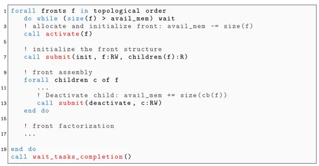
1 f o r a l l f r o n t s f in t o p o l o g i c a l o r d e r do w h i l e (s i z e( f ) > a v a i l _ m e m ) w a i t 3 ! a l l o c a t e and i n i t i a l i z e f r o n t : a v a i l _ m e m -= s i z e ( f ) c a l l a c t i v a t e( f ) 5 ! i n i t i a l i z e the f r o n t s t r u c t u r e 7 c a l l s u b m i t( init , f : RW , c h i l d r e n ( f ) : R ) 9 ! f r o n t a s s e m b l y f o r a l l c h i l d r e n c of f 11 ... ! D e a c t i v a t e c h i l d : a v a i l _ m e m += s i z e ( cb ( f ) ) 13 c a l l s u b m i t( d e a c t i v a t e , c : RW ) end do 15 ! f r o n t f a c t o r i z a t i o n 17 ... 19 end do c a l l w a i t _ t a s k s _ c o m p l e t i o n()
Fig. 7. Pseudo-code showing the implementation of the memory-aware tasks submission.
In our implementation this was achieved as shown in Figure 7. Before performing a front activation (line 4), the master thread, in charge of the tasks submission, checks if enough memory is available to perform the corresponding allocations (line 2). This
activation is a very lightweight operation which consists in simple memory bookkeep-ing (due to the first-touch rule) and therefore does not substantially slow down the tasks submission. The front structure is instead computed in a new init task (line 7) submitted to the runtime system which can potentially execute it on any worker thread.
5. EXPERIMENTAL RESULTS 5.1. Experimental setup
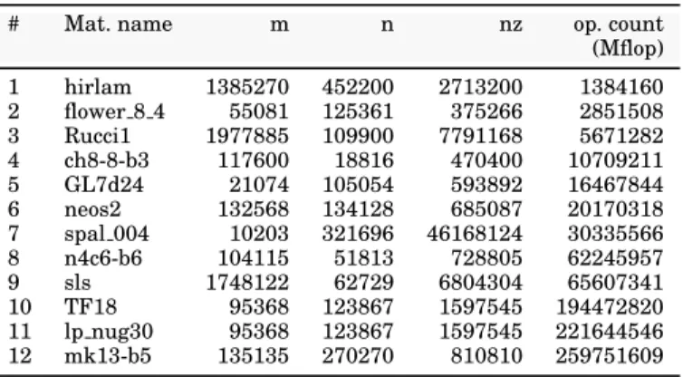
We evaluated the above discussed techniques and the code resulting from their imple-mentation on a set of eleven matrices from the UF Sparse Matrix Collection [Davis and Hu 2011] plus one (matrix #1) from the HIRLAM2research program. These matrices are listed in Table I along with their size, number of nonzeroes and operation count obtained when a nested dissection, fill-reducing column permutation is applied and a panel size of 32 is used for the factorization of fronts (this parameter defines how well the fronts staircase structure is exploited and thus affects the global operation count [Buttari 2013]); the column permutation is computed with the SCOTCH [Pel-legrini and Roman 1996] graph partitioning and ordering tool on the graph of ATA. In the case of under-determined systems, the transposed matrix is factorized, as it is commonly done to find the minimum-norm solution of a problem.
Table I. The set of matrices used for the experiments.
# Mat. name m n nz op. count
(Mflop) 1 hirlam 1385270 452200 2713200 1384160 2 flower 8 4 55081 125361 375266 2851508 3 Rucci1 1977885 109900 7791168 5671282 4 ch8-8-b3 117600 18816 470400 10709211 5 GL7d24 21074 105054 593892 16467844 6 neos2 132568 134128 685087 20170318 7 spal 004 10203 321696 46168124 30335566 8 n4c6-b6 104115 51813 728805 62245957 9 sls 1748122 62729 6804304 65607341 10 TF18 95368 123867 1597545 194472820 11 lp nug30 95368 123867 1597545 221644546 12 mk13-b5 135135 270270 810810 259751609
Experiments were done on one node of the ADA supercomputer installed at the IDRIS French supercomputing center3. This is an IBM x3750-M4 system equipped with four Intel Sandy Bridge E5-4650 (eight cores) processors and 128 GB of memory per node. The cores are clocked at 2.7 GHz and are equipped with Intel AVX SIMD units; the peak performance is of 21.6 Gflop/s per core and thus 691.2 Gflop/s per node for real, double precision computations (which is the arithmetic chosen for all our ex-periments).
Our code is written in Fortran20034, compiled with the Intel Compilers suite 2015; the code uses Intel MKL v11.2 BLAS and LAPACK routines, the SCOTCH ordering tool v6.0 and the trunk development version of the StarPU runtime system freely available through anonymous SVN access.
2http://hirlam.org 3http://www.idris.fr
In the experiments discussed below, local and interleaved memory allocation policies were used, respectively, for sequential and parallel runs through the use of the numactl tool; these are the policies that deliver the best performance in their respective cases.
For efficiently handling relatively low granularity tasks (especially in the 2D case), we have implemented a scheduling algorithm where each worker thread has its own queue of ready tasks, sorted by priority. Upon completion of a task, the executing worker pushes in its own queue all the newly executable tasks. When a worker runs out of tasks, a work-stealing mechanism is used where victims are selected depending on their distance in the memory hierarchy. This scheduler has been eventually inte-grated in the StarPU release and is now publicly available under the name lws (for locality work-stealing).
5.2. Performance and scalability of the 1D and 2D approaches
This section is meant to evaluate the performance of our code and, thus, we do not impose any memory constraint (the behavior of our memory-aware algorithm is ana-lyzed in Section 5.3). The purpose is to assess the usability and efficiency of runtime systems for complex, irregular workloads such as the QR factorization of a sparse ma-trix and to evaluate the effectiveness of parallel, 2D factorization algorithms in the multifrontal QR method. The reference sequential execution times are obtained with a purely sequential code (no potential runtime overhead) with no frontal matrix parti-tioning which ensures that all the LAPACK and BLAS routines execute at the maxi-mum possible speed (no granularity trade-off).
The performance of both parallel 1D and 2D methods depends on the choice of the values for a number of different parameters. For the 1D case these are the block-column nb on which depends the amount of concurrency and the internal block size ib on which depend the efficiency of elementary BLAS operations and the global amount of flop (this parameter defines how well the staircase structure of each front is ex-ploited). For the parallel 2D STF case these parameters are, the tiles size (mb,nb), the type of panel reduction algorithm set by the bh parameter described in Section 4.2 and the internal block size ib. The choice of these values depends on a number of factors, such as the number of working threads, the size and structure of the matrix, the shape of the elimination tree and of frontal matrices and the features of the underlying archi-tecture. It has to be noted that these parameters may be set to different values for each frontal matrix; moreover, it would be possible to let the software automatically choose values for these parameters. Both these tasks are very difficult and challenging and are out of the scope of this work. Therefore, for our experiments we performed a large number of runs with varying values for all these parameters, using the same values for all the fronts in the elimination tree, and selected the best results (shortest running time) among those. For the sequential runs internal block sizes ib={32, 40, 64, 80, 128} were used for a total of five runs per matrix. For the 1D parallel STF case, the used values were (nb,ib)={(128,32), (128,64), (128,128), (160,40), (160,80)} for a total of five runs per matrix. For the 2D case (nb,ib)={(160,32), (160,40), (192, 32), (192,64)}, mb={nb, nb*2, nb*3, nb*4} and bh={4, 8, 12, 16, 20, 24, ∞} for a total of 112 runs per matrix. This choice of values stems from the following observations. For the 1D case, tasks are of relatively coarse grain and, therefore, it is beneficial to choose smaller values for nb with respect to the 2D case in order to improve concurrency. On the other side, in the 2D case concurrency is aplenty and therefore it is beneficial to choose a relatively large nb value in order to achieve a bet-ter BLAS efficiency and keep the runtime overhead small; the inbet-ternal block size ib, however, has to be relatively small to keep the flop overhead under control.
All of the results presented in this section were produced without storing the fac-tors in order to extend the tests to the largest matrices in our experimental set that
could not otherwise be factorized (even in sequential) on the target platform. This was achieved by simply deallocating the tiles containing the factors coefficients at each deactivate task rather than keeping them in memory. As confirmed by experiments that we do not report here for the sake of space and readability, this does not have a relevant impact on the following performance analysis.
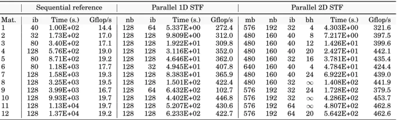
Table II. Optimum performance on ADA (32 cores).
Sequential reference Parallel 1D STF Parallel 2D STF
Mat. ib Time (s.) Gflop/s nb ib Time (s.) Gflop/s mb nb ib bh Time (s.) Gflop/s
1 40 1.00E+02 14.4 128 64 5.337E+00 272.4 576 192 32 4 4.303E+00 321.6
2 32 1.73E+02 17.0 128 128 9.809E+00 312.0 480 160 40 8 7.217E+00 397.5
3 80 3.40E+02 17.1 128 128 1.922E+01 309.8 480 160 40 12 1.426E+01 399.6
4 128 5.76E+02 19.0 128 128 3.116E+01 352.0 480 160 40 20 2.427E+01 442.1
5 80 8.71E+02 19.2 128 128 4.646E+01 362.0 480 160 32 16 3.781E+01 435.4
6 80 1.18E+03 17.7 128 32 4.945E+01 407.8 640 160 40 4 4.784E+01 424.4
7 128 1.58E+03 19.3 128 128 8.383E+01 365.9 480 160 40 24 6.922E+01 439.0
8 128 3.25E+03 19.5 128 128 1.501E+02 422.4 480 160 32 ∞ 1.408E+02 441.9
9 128 3.99E+03 16.7 128 64 6.432E+02 102.7 576 192 32 24 1.728E+02 379.5
10 128 9.93E+03 19.7 128 128 4.402E+02 446.8 576 192 32 ∞ 4.286E+02 453.7
11 128 1.13E+04 19.7 128 128 5.207E+02 430.6 576 192 64 ∞ 4.807E+02 462.8
12 128 1.37E+04 19.2 128 128 6.233E+02 422.7 576 192 64 20 5.642E+02 462.6
Table II shows for both the 1D and 2D algorithms the parameter values deliver-ing the shortest execution time along with the corresponddeliver-ing attained factorization time and Gflop rate. The Gflop rates reported in the table are related to the operation count achieved with the internal block size ib reported therein without including, for the 2D case, the extra flops due to the 2D algorithm; these are difficult to count and can simply be regarded as a price to pay to achieve better concurrency (more exper-imental analysis of this extra-cost are provided below). For the 1D case, the smaller block-column size of 128 always delivers better performance because it offers a better compromise between concurrency and efficiency of BLAS operations, whereas a large internal block size is more desirable because it leads to better BLAS speed despite a worse exploitation of the fronts staircase structure. For the 2D case it is interesting to note that the shortest execution time is never attained with square tiles; this is likely because rectangular tiles lead to a better compromise between granularity of tasks (and, thus, efficiency of operations) and concurrency. The best speed of 462.8 Gflop/s is achieved for matrix #11, which corresponds to 67% of the system peak performance.
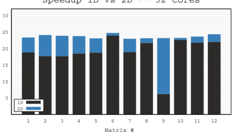
Figure 8, generated with the timing data in Table II, shows the speedup achieved by the 1D and 2D parallel codes with respect to the sequential one when using all the 32 cores available on the system. This figure shows that the 2D algorithms provide better gains on smaller size matrices or on those where frontal matrices are extremely overdetermined (which is the case for matrix #9) where the 1D method does not pro-vide enough concurrency; on larger size matrices the difference between the two par-allelization strategies decreases as the 1D approach achieves very good performance. The average speedup achieved by the 2D code is 23.61 with a standard deviation of 0.53, reaching a maximum of 24.71 for matrix #6. For the 1D case, instead, the av-erage is 19.04 with a standard deviation of 4.55. In conclusion, the 2D code achieves better and more consistent scalability over our heterogeneous set of matrices.
As in our previous runtime based approach [Agullo et al. 2013], we evaluate the performance of our implementation by means of efficiency measures based on the cu-mulative time spent inside tasks tt(p), the cumulative time spent by workers in the runtime system tr(p) and the cumulative time spent idle ti(p), p being the number of threads; these time measurements are provided by the StarPU runtime system. The
5 10 15 20 25 30 1 2 3 4 5 6 7 8 9 10 11 12 Matrix # Speedup 1D vs 2D -- 32 cores 1D 2D
Fig. 8. Speedup of the 1D and 2D algorithms with respect to the sequential case on ADA (32 cores).
efficiency e(p) of the parallelization can then be defined in terms of these cumulative timings as follows: e(p) = tt(1) tt(p) + tr(p) + ti(p) = eg tt(1) tt(˜1) · el tt(˜1) tt(p) · er tt(p) tt(p) + tr(p) · es tt(p) + tr(p) tt(p) + tr(p) + ti(p) where tt(˜1) is the time spent inside tasks when the parallel (either 1D or 2D) code is run with only one worker thread. This expression allows us to decompose the efficiency as the product of four well identified effects:
— eg: the granularity efficiency which measures how the overall efficiency is re-duced by the data partitioning and the use of parallel (either 1D or 2D) algorithms. This loss of efficiency is mainly due to the fact that because of the partitioning of data into fine grained tiles BLAS operation do not run at the same speed as in the purely sequential code. Moreover, 2D factorization algorithms induce an extra cost in terms of floating-point operations [Buttari et al. 2009]; this overhead may be re-duced by choosing an appropriate inner blocking size for the kernels but cannot, in general, be considered negligible.
— el: the locality efficiency which measures whether and how the execution of tasks was slowed-down by parallelism. This is due to the fact that our target system is a NUMA architecture and, therefore, the concurrent execution of tasks may suffer from a reduced memory bandwidth and from memory access contention.
— er: the runtime efficiency, which measures the cost of the runtime system with respect to the actual work done.
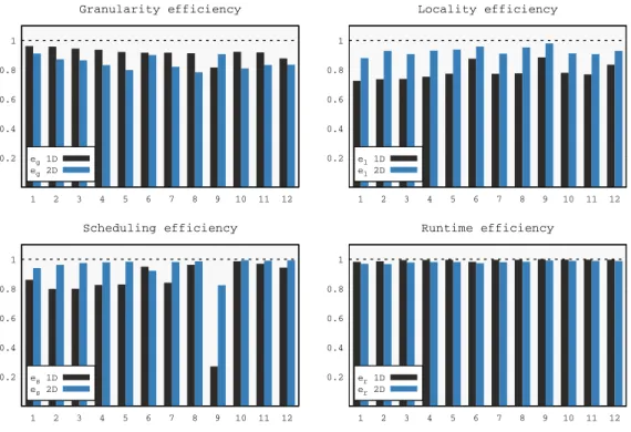
— es: the scheduling efficiency, which measures how well the tasks have been pipelined. This includes two effects. First, the quality of the scheduling because if the scheduling policy takes bad decisions (for example, it delays the execution of tasks along the critical path) many stalls can be introduced in the pipeline. Second, the shape of the DAG or, more generally, the amount of concurrency it delivers: for example, in the extreme case where the DAG is a chain of tasks, any scheduling policy will do as bad because all the workers except one will be idling at any time. Figure 9 shows a comparison of the four efficiency measures for the 1D and 2D algorithms. The 2D algorithms obviously have a lower granularity efficiency because of the smaller granularity of tasks and because of the extra flops. Note that the 1D
0.2 0.4 0.6 0.8 1 1 2 3 4 5 6 7 8 9 10 11 12 Granularity efficiency eg 1D eg 2D 0.2 0.4 0.6 0.8 1 1 2 3 4 5 6 7 8 9 10 11 12 Locality efficiency el 1D el 2D 0.2 0.4 0.6 0.8 1 1 2 3 4 5 6 7 8 9 10 11 12 Scheduling efficiency es 1D es 2D 0.2 0.4 0.6 0.8 1 1 2 3 4 5 6 7 8 9 10 11 12 Runtime efficiency er 1D er 2D
Fig. 9. Efficiency measures on ADA (32 cores).
code may suffer from a poor cache behavior in the case of extremely overdetermined frontal matrices because of the extremely tall-and-skinny shape of block-columns. This explains why the granularity efficiency for the 2D code on matrix #9 is better than for the 1D code unlike for the other matrices: most of the flops in this matrix are in one front with roughly 1.3 M rows and only 7 K columns. 2D algorithms, however, achieve better locality efficiency than 1D most likely due to the 2D partitioning of frontal matrices into tiles which have a more cache-friendly shape than the extremely tall and skinny block-columns used in the 1D algorithm. Not surprisingly, the 2D code achieves much better scheduling efficiency (i.e., less idle time) than the 1D code on all matrices: this results from a much higher concurrency, which is the purpose of the 2D code. As for the runtime efficiency, it is in favor of the 1D implementation due to a much smaller number of tasks with bigger granularity and simpler dependencies. However the performance loss induced by the runtime is extremely small in both cases: less than 2% on average and never higher than 4% for the 2D implementation, showing the efficiency of our lws scheduling strategy for dealing with tasks of small granularity.
5.3. Performance under a memory constraint
This section describes and analyses experiments that aim at assessing the effective-ness of the memory aware scheduling presented in Section 4.4. Here we are interested in two scenarios:
(1) In-Core (IC) execution: this is the most common case where the computed factors are kept in memory. In this case matrices #11 and #12 could not be used because of the excessive memory consumption.
(2) Out-Of-Core (OOC) execution: in this scenario the factors are written to disk as they are computed in order to save memory. In this case the memory consumption is more irregular and more considerably increased by parallelism. We simulate this scenario by discarding the factors as we did in the previous section; note that by doing so we are assuming that the overhead of writing data to disk has a negligible effect on the experimental analysis reported here.
These experiments were meant to measure the performance of both the 1D and 2D factorization (with the parameter values in Table II) within an imposed memory foot-print; experiments were performed using 32 cores with memory constraints equal to {1.0, 1.2, 1.4, 1.6, 1.8, 2.0} × sequential peak both when the factors are kept in memory and when they are discarded.
For all 1D and 2D IC tests as well as all 2D OOC tests, a performance as high as the non constrained case (such as discussed in Section 5.2) could be achieved with a memory exactly equal to the sequential peak, which is the lower bound that a par-allel execution can achieve. This shows the extreme efficiency of the memory-aware mechanism for achieving high-performance within a limited memory footprint. Com-bined with the 2D numerical scheme, the memory-aware algorithm is thus extremely robust since it could process all considered matrices at maximum pace with the mini-mum possible memory consumption. The only cases which requested a higher memory usage for achieving the same performance as the non constrained algorithm were for matrices #1 and #7 in the 1D OOC case.
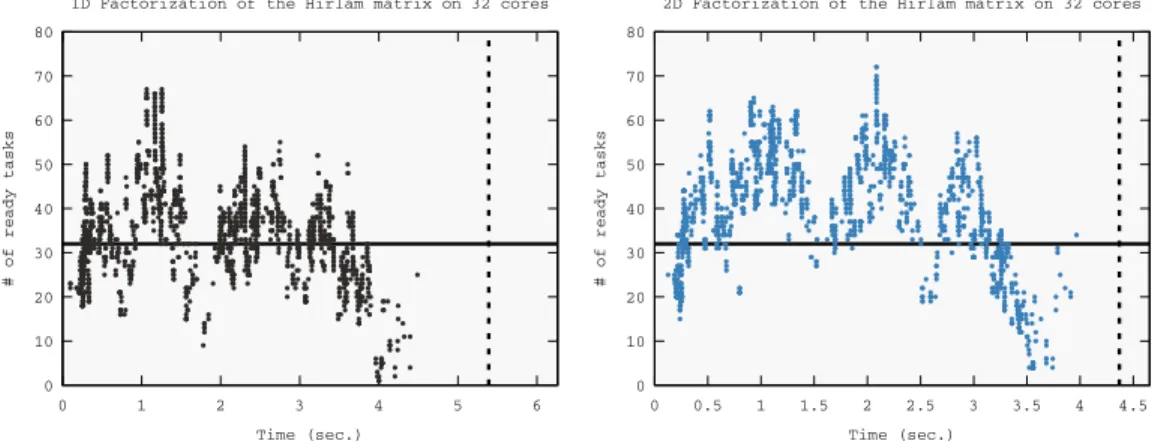
To explain this extreme efficiency, we performed the following analysis. As explained in Section 4.4, prior to activating a front, the master thread checks whether enough memory is available to achieve this operation. If it is not the case, the master thread is put to sleep and later woken up as soon as one deactivate task is executed; at this time the master thread checks again for the availability of memory. The master thread stays in this loop until enough deactivation tasks have been executed to free up the memory needed to proceed with the next front activation. Every time the master thread was suspended or resumed we recorded the time stamp and the number of ready tasks (i.e., those whose dependencies were all satisfied).
0 10 20 30 40 50 60 70 80 0 1 2 3 4 5 6 # of ready tasks Time (sec.)
1D Factorization of the Hirlam matrix on 32 cores
0 10 20 30 40 50 60 70 80 0 0.5 1 1.5 2 2.5 3 3.5 4 4.5 # of ready tasks Time (sec.)
2D Factorization of the Hirlam matrix on 32 cores
Fig. 10. Concurrency under a memory constraint for the Hirlam matrix on ADA (32 cores).
Figure 10 shows the collected data for the Hirlam matrix with an imposed memory consumption equal to the sequential peak, in the OOC case using both the 1D (left)
and 2D (right) methods. In this figure, each (x, y) point means that at time x the mas-ter thread was suspended or resumed and that, at that time, y tasks where ready for execution or being executed. The width of each graph shows the execution time of the memory constrained factorization whereas the vertical dashed line shows the execu-tion time when no limit on the memory consumpexecu-tion is imposed. The figure leads to the following observations:
— in both the 1D and 2D factorizations, the number of ready tasks falls, at some point, below the number of available cores (the horizontal, solid line); this lack of tasks is responsible for a longer execution time with respect to the unconstrained case. — in the 1D factorization this lack of tasks is more important; this can be explained
by the fact that the 1D method delivers much lower concurrency than the 2D one and therefore, suspending the submission of tasks may lead more quickly to thread starvation. As a result, the difference in the execution times of the constrained and unconstrained executions is more evident in the 1D factorization.
For the 1D, OOC factorization of matrix #7, the performance increases smoothly when the memory constraint is gradually increased as described above. The corre-sponding execution times are: 126.7, 118.3, 116.1, 114.9, 94.7, 93.0 seconds.
For all other tests, either the number of tasks is always (much) higher than the num-ber of used cores or the tasks submission is never (or almost never) interrupted due to the lack of memory; as a result, no relevant performance degradation was observed with respect to the case where no memory constraint is imposed. This behavior mainly results from two properties of the multifrontal QR factorization. First, the size of the contribution blocks is normally very small compared to the size of factors, especially in the case where frontal matrices are overdetermined. Second, the size of a front is always greater than or equal to the sum of the sizes of all the contribution blocks as-sociated with its children (because in the assembly operation, contribution blocks are not summed to each other but stacked). As a result, in the sequential multifrontal QR factorization, the memory consumption grows almost monotonically and in most cases the sequential peak is achieved on the root node or very close to it. For this reason, when the tasks submission is interrupted in a memory-constrained execution, a large portion of the elimination tree has already been submitted and the number of avail-able tasks is considerably larger than the number of working threads. We expect that other types of multifrontal factorizations (LU , for instance) are more sensitive to the memory constraint because they do not possess the two properties described above. By the same token, it is reasonable to expect that imposing a memory constraint could more adversely affect performance when larger numbers of threads are used.
6. CONCLUSIONS
With this work we aimed at assessing the usability and effectiveness, in a shared-memory environment, of modern runtime systems for handling a complex, irregular workload such as the multifrontal QR factorization of a sparse matrix which is char-acterized by a very high number of extremely heterogeneous tasks with complex de-pendencies. We showed how to use the Sequential Task Flow programming model to implement the parallelization approach presented in our previous work [Buttari 2013] for such method; this model leads to a simpler, more portable, maintainable, and scal-able code. We showed how the resulting code could be improved with a relatively lim-ited effort thanks to the simplicity of the STF programming model. First, we addressed the performance scalability issues of the 1D parallel approach by implementing com-munication avoiding fronts factorization by tiles. Second, we presented an approach that, by simply controlling the submission of tasks to the runtime system, allows for achieving the factorization within a prescribed memory footprint.
We presented experimental results that assess the effectiveness of our approach by showing that modern runtime systems are very lightweight and efficient, that tile, communication-avoiding parallel algorithms provide better concurrency and scalabil-ity to the multifrontal QR factorization and that the memory consumption of this method can be simply yet effectively controlled without introducing a performance penalty in nearly all of the considered test cases. In conclusion, the resulting code achieves a great performance and scalability as well as an excellent robustness when it comes to memory consumption. The present work can also be viewed as an important contribution to bridge the gap between theoretical results [Eyraud-Dubois et al. 2015] and actual implementation within modern sparse direct solver. We proved that rely-ing on STF and fully-featured runtime systems is a solid way for achievrely-ing this goal. Finally, this study can also induce the runtime community to integrate memory-aware mechanisms directly within the runtime systems; in particular, the StarPU team has now done so, which would be of great value for many users.
7. ACKNOWLEDGMENTS
We wish to thank the RUNTIME team of Inria Bordeaux sud-ouest for their help in using the StarPU runtime system and for promptly addressing our requests. We also thank B. Liz´e and M. Faverge as well as the reviewers for their constructive sugges-tions on a preliminary version of this manuscript.
REFERENCES
Emmanuel Agullo, Alfredo Buttari, Abdou Guermouche, and Florent Lopez. 2013. Multifrontal QR Fac-torization for Multicore Architectures over Runtime Systems. In Euro-Par 2013 Parallel Processing. Springer Berlin Heidelberg, 521–532.http://dx.doi.org/10.1007/978-3-642-40047-6 53
Emmanuel Agullo, Jim Demmel, Jack Dongarra, Bilel Hadri, Jakub Kurzak, Julien Langou, Hatem Ltaief, Piotr Luszczek, and Stanimire Tomov. 2009. Numerical linear algebra on emerging architectures: The PLASMA and MAGMA projects. Journal of Physics: Conference Series 180, 1 (2009), 012037. http:// stacks.iop.org/1742-6596/180/i=1/a=012037
Emmanuel Agullo, Jack Dongarra, Rajib Nath, and Stanimire Tomov. 2011. Fully Empirical Autotuned QR Factorization For Multicore Architectures. CoRR abs/1102.5328 (2011).
Randy Allen and Ken Kennedy. 2002. Optimizing Compilers for Modern Architectures: A Dependence-Based Approach. Morgan Kaufmann.
Patrick R. Amestoy, Iain S. Duff, and Chiara Puglisi. 1996. Multifrontal QR factorization in a multiprocessor environment. Int. Journal of Num. Linear Alg. and Appl. 3(4) (1996), 275–300.
The OpenMP architecture review board. 2013. OpenMP 4.0 Complete specifications. (2013).
Nimar S. Arora, Robert D. Blumofe, and C. Greg Plaxton. 2001. Thread Scheduling
for Multiprogrammed Multiprocessors. Theory Comput. Syst. 34, 2 (2001), 115–144.
DOI:http://dx.doi.org/10.1007/s00224-001-0004-z
Cedric Augonnet, Samuel Thibault, Raymond Namyst, and Pierre-Andr´e Wacrenier. 2011. StarPU: A Unified Platform for Task Scheduling on Heterogeneous Multicore Architectures. Concurrency and Computation: Practice and Experience, Special Issue: Euro-Par 2009 23 (Feb. 2011), 187–198. DOI:http://dx.doi.org/10.1002/cpe.1631
Rosa M. Badia, Jos´e R. Herrero, Jes ´us Labarta, Josep M. P´erez, Enrique S. Quintana-Ort´ı, and Gregorio Quintana-Ort´ı. 2009. Parallelizing dense and banded linear algebra libraries using SMPSs. Concurrency and Computation: Practice and Experience 21, 18 (2009), 2438–2456.
George Bosilca, Aurelien Bouteiller, Anthony Danalis, Thomas H´erault, Pierre Lemarinier, and Jack Don-garra. 2012. DAGuE: A generic distributed DAG engine for High Performance Computing. Parallel Comput. 38, 1-2 (2012), 37–51. DOI:http://dx.doi.org/10.1016/j.parco.2011.10.003
George Bosilca, Aurelien Bouteiller, Anthony Danalis, Thomas Herault, Piotr Luszczek, and Jack Dongarra. 2013. Dense Linear Algebra on Distributed Heterogeneous Hardware with a Symbolic DAG Approach. Scalable Computing and Communications: Theory and Practice (2013), 699–733.
Henricus Bouwmeester, Mathias Jacquelin, Julien Langou, and Yves Robert. 2011. Tiled QR Fac-torization Algorithms. In Proceedings of 2011 International Conference for High Performance Computing, Networking, Storage and Analysis (SC ’11). ACM, New York, NY, USA, 7:1–7:11. DOI:http://dx.doi.org/10.1145/2063384.2063393