Computer optimization of dry and wet/dry cooling tower systems for large fossil and nuclear power plants

SYSTEMS FOR LARGE FOSSIL AND NUCLEAR POWER PLANTS by

Michael Choi and Leon R. Glicksman Energy Laboratory Report No. MIT-EL 79-034

COMPUTER OPTIMIZATION OF DRY AND WET/DRY COOLING TOWER SYSTEMS FOR LARGE FOSSIL AND NUCLEAR POWER PLANTS

by Michael Choi and Leon R. Glicksman Energy Laboratory and

Heat Transfer Laboratory

Department of Mechanical Engineering Massachusetts Institute of Technology

Cambridge, Massachusetts 02139

Prepared under the support of the Environmental Control Technology Division

Office of the Assistant Secretary for the Environment

U.S. Department of Energy Contract No. EY-76-S-02-4114.A001

Energy Laboratory Reporc No. MIT-EL 79-034

ABSTRACT

There is a projected shortage of water supply for evaporative cooling in electric power industry by the end of this century. Thus, dry and

wet/dry cooling tower systems are going to be the solution for this problem. This study has determined the cost of dry cooling compared to the conventional cooling methods. Also, the savings by using wet/dry instead of all-dry cooling has been determined.

A total optimization has been performed for power plants with dry cooling tower systems using metal-finned-tube heat exchangers and surface condensers. The optimization minimizes the power production cost.

The program does not use pre-designed heat exchanger modules. Rather, it optimizes the heat exchanger and its air and water flow rates.

In the base case study, the method of replacing lost capacity assumes the use of gas turbines. As a result of using dry cooling towers in an 800 MWe fossil plant, the incremental costs with the use of high back pressure turbine and conventional turbine over all-wet cooling are 11% and 15%, respectively. For a 1200 MWe nuclear plant, these are 22% and 25%, respectively.

Since the method of making up lost capacity depends on the situation of a utility, considerable effort has been placed on testing the effects of using different methods of replacing lost capacity at high ambient

temperatures by purchased energy. The results indicate that the optimization is very sensitive to the method of making up lost capacity. It is, there-fore, important to do an accurate representation of all possible methods of making up capacity loss when optimizating power plants with dry cooling towers.

A solution for the problem of losing generation capability by a power plant due to the use of a dry cooling tower is to supplement the

dry tower during the hours of peak ambient temperatures by a wet tower. A separate wet/dry cooling tower system with series tower arrangement has been considered in this study. In this cooling system, the physical separation of the dry and wet towers protects the dry tower airside heat

transfer surface from the corrosion problem. It also allows complete freedom of design and operation of the dry and wet towers. A wet/dry cooling system can be tailored to meet any amount of water available for cooling. The results of the optimization show that wet/dry cooling towers have significant savings over all-dry cooling. For example, in either

fossil or nuclear plant, the dry tower heat transfer surface of 30% makeup water wet/dry cooling system is only about fifty percent of that in all-dry

cooling using high back pressure turbines. This results in a reduction of 27% and 37% of the incremental cost in the fossil and nuclear plant,

respectively, over all-wet cooling. Even the availability of a small percentage of makeup water reduces the incremental cost significantly. Thus, wet/dry cooling is an economic choice over all-dry cooling where some water is available but supplies are insufficient for a totally evaporative

cooling towers. On the other hand, the advantage of wet/dry cooling over evaporative towers is conservation of water consumption.

-3-ACKNOWLEDGMENTS

This report is part of an interdisciplinary effort by the MIT Energy Laboratory to examine issues of power plant cooling system design

and operation under environmental constraints. The effort has involved participation by researchers in the R.M. Parsons Laboratory for Water Resources and Hydrodynamics of the Civil Engineering Department and the Heat Transfer Laboratory of the Mechanical Engineering Department. Financial support for this research effort has been provided by the

Division of Environmental Control Technology, U.S. Dept. of Energy, under Contract No. EY-76-S-02-4114.AOO1. The assistance of Dr. William Mott,

Dr. Myron Gottlieb and Mr. Charles Grua of DOE/ECT is gratefully acknowledged. Reports published under this sponsorship include:

"Computer Optimization of Dry and Wet/Dry Cooling Tower Systems for Large Fossil and Nuclear Plants," by Choi, M., and

Glicksman, L.R., MIT Energy Laboratory Report No. MIT-EL 79-034, February 1979.

"Computer Optimization of the MIT Advanced Wet/Dry Cooling Tower Concept for Power Plants," by Choi, M., and Glicksman, L.R., MIT Energy Laboratory Report No. MIT-EL 79-035, September 1979.

"Operational Issues Involving Use of Supplementary Cooling Towers to Meet Stream Temperature Standards with Application to the

Browns Ferry Nuclear Plant," by Stolzenbach, K.D., Freudberg, S.A., Ostrowski, P., and Rhodes, J.A., MIT Energy Laboratory Report No. MIT-EL 79-036, January 1979.

"An Environmental and Economic Comparison of Cooling System

Designs for Steam-Electric Power Plants," by Najjar, K.F., Shaw, JJ., Adams, E.E., Jirka, G.H., and Harleman, D.R.F,, MIT Energy

Laboratory Report No. MIT-EL 79-037, January 1979.

"Economic Implications of Open versus Closed Cycle Cooling for New Steam-Electric Power Plants: A ational and Regional Survey," by Shaw, J.J., Adams, E.E., Barbera, R.J., Arntzen, B.C,, and Harleman, D.R.F., MIT Energy Laboratory Report No. MIT-EL 79-038, September 1979.

"Mathematical Predictive Models for Cooling Ponds and Lakes," Part B: User's Manual and Applications of MITEMP by Octavio, K.H., Watanabe, M., Adams, E.E., Jirka, G.H., Helfrich, K.R., and

Harleman, D.R.F.; and Part C A Transient Analytical Model for Shallow Cooling Ponds, by Adams, E.E., and Koussis, A., MIT Energy Laboratory Report No. MIT-EL 79-039, December 1979.

"Summary Report of Waste Heat Management in the Electric Power Industry: Issues of Energy Conservation and Station Operation under Environmental Constraints," by Adams, E.E., and Harleman, D.R.F., MIT Energy Laboratory Report N. MIT-EL 79-040, December 1979.

TABLE OF CONTENTS Page Abstract . . . . Acknowledgements . . . . List of Figures . . . . List of Tables . . . . CHAPTER 1: INTRODUCTION . . . . 1.1 Background . . . . 1.2 Scope of This Thesis Work 1.3 Outline of Presentation

CHAPTER 2: APPROACH AND MAJOR ASSUMPTIONS . 2.1 Introduction . . . . 2.2 Optimum System . . . . 2.3 Load Profile . . . . 2.4 Treatment of Loss of Capacity . . 2.5 Power Production Cost . . . . 2.6 Base Economic Factors . . . . CHAPTER 3: CHARACTERISTICS OF THE POWER PLANT

3.1 3.2 CHAPTER 4 4.1 4.2 4.3 4.4 4.5 Plant Model . . . Turbines . . . . . : DRY COOLING TOWER

Introduction . . . Condenser . . . . Dry Towers . . . . Piping System . . Pumping System . . * . . . .* * . . . .*

SYSTEM MODEL AND

. . . . .* * . . . I * . . . . * . . . . . . . . ·. . . . . .PER.OR ... . . . . . . . . . .* . . . . . . . . * . . . . . . . . . itPERFORMANCE ... . . . . . . . . . . . . * . . . . * . . . .*

CHAPTER 5: OPTIMIZATION OF DRY COOLING TOWER SYSTEMS AND RESULTS 5.1 Introduction . . . . 5.2 Dry Cooling Tower Optimization Procedure . . . . 5.3 Results of Dry Cooling Tower Optimization . . . .

2 3 8 12 14 14 16 17 18 18 18 21 21 22 23 24 24 25 32 32 34 43 49 52 53 53 55 58 . . . . . . . . . . . . . . . .

CHAPTER 6: THE EFFECTS OF DIFFERENT METHODS OF REPLACING LOST CAPACITY ON THE ECONOMIC OPTIMIZATION OF

DRY COOLING TOWER SYSTEMS . . . 79

6.1 Introduction . . . 79

6.2 Approach to the Problem . . . 79

6.3 Results . . . 81

6.4 Discussion . . . 82

CHAPTER 7: WET/DRY COOLING TOWER SYSTEM: MODEL, OPTIMIZATION, AND RESULTS ... 90

7.1 Introduction . . . 90

7.2 Tower Arrangement and Operating Scheme . . . 91

7.3 Wet Tower Model and Performance . . . 91

7.4 Computation of Makeup Water Requirement . . . 100

7.5 Wet Tower Cost ... 102

7.6 Optimization Procedure . . . 103

7.7 Results of Wet/Dry Cooling Tower System Optimization . 104 CHAPTER 8: COMPARISON OF ECONOMICS OF DRY AND WET/DRY COOLING TOWER SYSTEMS WITH ONCE-THROUGH, COOLING POND, AND EVAPORATIVE TOWERS . . . 119

8.1 Economic Comparison of Base Case Study . . . 119

8.2 Economic Comparison of Sensitivity Study . . . 119

CHAPTER 9: CONCLUSIONS AND RECOMMENDATIONS . . . 137

9.1 Conclusions . . . 137

9.2 Comparison to Previous Work and Other Published Studies 138 9.3 Recommendations . . . 143

References ... ... 144

APPENDIX I: Equations for Calculating Hydraulic Pressure Drop . . 147

APPENDIX II: Cooling System Cost Models . . . . .. . . . 148

APPENDIX III: Piping Water Velocity Optimization . . . 162

APPENDIX IV: Dry Tower Heat Exchanger Specifications . . . 167

Page

APPENDIX VI: Condenser Specifications . . . 169

APPENDIX VII: Computer Program Listing For Dry Cooling

Tower System ... 170

APPENDIX VIII: Computer Program Listing for Wet/Dry

Cooling Tower System Optimization . . . 215

LIST OF FIGURES Page FIGURE 2.1 FIGURE 2.2 FIGURE 3.1 FIGURE 3.2 FIGURE 4.1 FIGURE 4.2 FIGURE 4.3 FIGURE 4.4 FIGURE 5.1 FIGURE 5.2 FIGURE 5.3 FIGURE 5.4 FIGURE 5.5 FIGURE 5.6

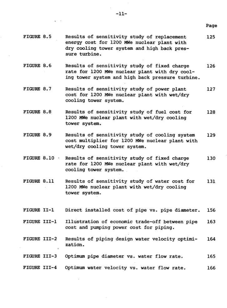
Illustration of the concept of power plant scaling.

Illustration of economic trade-off between capital cost and operating cost.

Nuclear turbine heat rate characteristic curves.

Fossil turbine heat rate characteristic curves.

Indirect type of mechanical draft dry cooling tower system.

Temperature relationship in indirect type of dry cooling tower system.

Piping layout in dry cooling tower system. Dry tower piping.

Illustration of Andeen-Glicksman minimization technique.

Power production cost vs. design ITD for 800 MWe fossil plant with dry cooling tower system and conventional turbine.

Power production cost vs. design ITD for 800 MWe fossil plant with dry cooling tower system and high back pressure turbine.

Power production cost vs. design ITD for 1200 MWe nuclear plant with dry cooling tower system and

conventional turbine.

Power production cost vs. design TID for 1200 MWe nuclear plant with dry cooling tower system and high back pressure turbine.

Power production cost breakdown vs. design ITD for 800 MWe fossil plant with dry cooling tower system and conventional turbine.

19 20 26 27 33 35 50 51 61 62 63 64 65 66

Page FIGURE 5.7 FIGURE 5.8 FIGURE 5.9 FIGURE 5.10 FIGURE 5.11 FIGURE 6.1 FIGURE 6.2 FIGURE 6.3 FIGURE 6.4 FIGURE 7.1 FIGURE 7.2 FIGURE 7.3

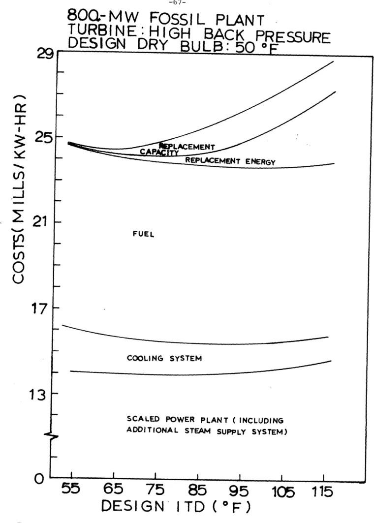
Power production cost breakdown vs. design TD for 800 MWe fossil plant with dry cooling tower system and high back pressure turbine.

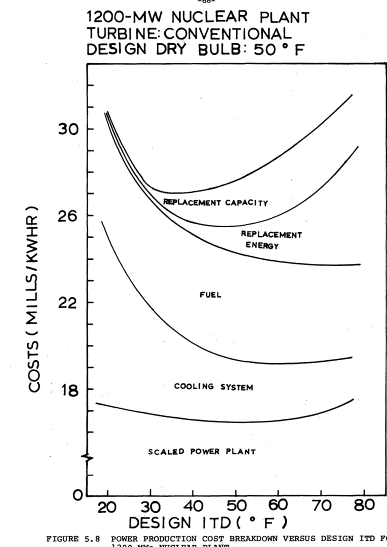
Power production cost breakdown vs. design ITD for 1200 MWe nuclear plant with dry cooling tower system and conventional turbine.

Power production cost breakdown vs. design ITD for 1200 MWe nuclear plant with dry cooling tower system and high back pressure turbine. Total capital cost of dry cooling tower system vs. design ITD for conventional turbine.

Total capital cost of dry cooling tower system vs. design ITD for high back pressure turbine.

Results of optimization using different methods of replacing lost capacity for 800 MWe fossil plant with dry cooling tower system and conven-tional turbine.

Results of optimization using different methods of replacing lost capacity for 800 MWe fossil plant with dry cooling tower system and high back pressure turbine.

Results of optimization using different methods of replacing lost capacity for 1200 MWe nuclear plant with dry cooling tower system and conven-tional turbine.

Results of optimization using different methods of replacing lost capacity for 1200 MWe nuclear plant with dry cooling tower system and high back pressure turbine.

Water flow diagram for wet/dry cooling tower system.

Operating scheme of wet/dry cooling tower system. Illustration of towc'

fi!

finite different cal-culation. 67 68 69 70 71 83 84 85 86 92 92 94

FIGURE 7.4 FIGURE 7.5 FIGURE 7.6 FIGURE 7.7 FIGURE 7.8 FIGURE 7.9 FIGURE 7.10 FIGURE 7.11 FIGURE 7.12 FIGURE 8.1 FIGURE 8.2 FIGURE 8.3 FIGURE 8.4

Schematization of elementary volume within tower fill.

Power production cost vs. annual makeup water quantity for 800 MWe fossil plant.

Direct capital cost of cooling system vs. annual makeup water quantity for 800 MWe fossil plant. Wet tower size vs. annual makeup water quantity

for 800 MWe fossil plant.

Instantaneous makeup water consumption rate at maximum ambient vs. wet tower size for 800 MWe fossil plant.

Power production cost vs. annual makeup water quantity for 1200 MWe nuclear plant.

Direct capital cost of cooling system vs. annual makeup water quantity for 1200 MWe nuclear plant.

Wet tower size vs. annual makeup water quantity for 1200 MWe nuclear plant.

Instantaneous makeup water consumption rate at maximum ambient vs. wet tower size for 1200 MWe nuclear plant.

Results of sensitivity study of power plant cost for 1200 MWe nuclear plant with dry cooling tower system and high back pressure turbine.

Results of sensitivity study of fuel cost for 1200 MWe nuclear plant with dry cooling tower system and high back pressure turbine.

Results of sensitivity study of cooling system cost multiplier for 1200 MWe nuclear plant with dry cooling tower system and high back pressure turbine.

Results of sensitivity study of replacement capacity cost for 1200 MWe nuclear plant with dry cooling tower system and high back pressure turbine. 99 107 108 109 110 111 112 113 114 121 122 123 124

Page FIGURE 8.5 FIGURE 8.6 FIGURE 8.7 FIGURE 8.8 FIGURE 8.9 FIGURE 8.10 FIGURE 8.11 FIGURE II-1 FIGURE III-1 FIGURE III-2 FIGURE III-3

Results of sensitivity study of replacement energy cost for 1200 MWe nuclear plant with dry cooling tower system and high back

pres-sure turbine.

Results of sensitivity study of fixed charge rate for 1200 MWe nuclear plant with dry cool-ing tower system and high back pressure turbine. Results of sensitivity study of power plant cost for 1200 MWe nuclear plant with wet/dry cooling tower system.

Results of sensitivity study of fuel cost for 1200 MWe nuclear plant with wet/dry cooling tower system.

Results of sensitivity study of cooling system cost multiplier for 1200 MWe nuclear plant with wet/dry cooling tower system.

Results of sensitivity study of fixed charge rate for 1200 MWe nuclear plant with wet/dry cooling tower system.

Results of sensitivity study of water cost for 1200 MWe nuclear plant with wet/dry cooling tower system.

Direct installed cost of pipe vs. pipe diameter. Illustration of economic trade-off between pipe cost and pumping power cost for piping.

Results of piping design water velocity optimi-zation.

Optimum pipe diameter vs. water flow rate. Optimum water velocity vs. water flow rate.

125 126 127 128 129 130 131 156 163 164 165 FIGURE III-4 166

LIST OF TABLES

Base case study of economic parameters.

Nuclear turbine net heat rates.

Fossil turbine net heat rates.

Condenser heat transfer coefficient vs. water velocity.

Comparison of condenser heat transfer coeffi-cients obtained by Nusselt analysis and empirical correlation given by Heat Exchange Institute.

Optimum design parameters of dry cooling tower systems for 800 MWe fossil plant.

Optimum design parameters of dry cooling tower systems for 1200 MWe nuclear plant.

Cost comparison of optimum design dry cooling tower systems for 800 MWe fossil plant.

Cost comparison of optimum design dry cooling tower systems for 1200 MWe nuclear plant.

800 MWe fossil plant net electrical output for optimum cooling system design.

1200 MWe nuclear plant net electrical output for optimum cooling system design.

Comparison of heat exchanger tube length and number of tubes deep for 1200 MWe nuclear plant.

Comparison of heat exchanger tube length and number of tubes deep for 800 MWe fossil plant.

Optimum dry tower design ITD using different methods of replacing lost capacity.

Optimum power generation cost using different methods of replacing lost capacity.

800 MWe dry-cooled fossil plant net electrical output vs. ambient temperature.

Page 23 29 30 38 39 72 73 74 75 76 77 78 78 87 87 88 TABLE 2.1 TABLE 3.1 TABLE 3.2 TABLE 4.1 TABLE 4.2 TABLE 5.1 TABLE 5.2 TABLE 5.3 TABLE 5.4 TABLE 5.5 TABLE 5.6 TABLE 5.7 TABLE 5.8 TABLE 6.1 TABLE 6.2 TABLE 6.3

page TABLE 6.4 TABLE 7.1 TABLE 7.2 TABLE 7.3 TABLE 7.4 TABLE 8.1 TABLE 8.2 TABLE 8.3 TABLE 8.4 TABLE 8.5 TABLE 8.6 TABLE 9.1 TABLE 9.2 TABLE II-1

1200 MWe dry-cooled nuclear plant net electrical output vs. ambient temperature.

Comparison of two different optimum design wet/dry cooling tower systems for 800 MWe fossil plant.

89

115

116 Comparison of two different optimum design

wet/dry cooling tower systems for 1200 MWe nuclear plant.

Comparison of capital cost breakdowns of dry and 117 wet/dry cooling tower systems for 1200 MWe nuclear plant.

Comparison of capital cost breakdowns of dry and wet/dry cooling tower systems for 800 MWe fossil plant.

Economic comparison of base case study optimum design cooling systems for 800 MWe fossil plant. Economic comparison of base case study optimum design cooling systems for 1200 MWe nuclear plant. Economic comparison of sensitivity study optimum design cooling systems for 800 MWe fossil plant. Economic comparison of sensitivity study optimum design cooling system for 1200 MWe nuclear plant. Comparison of incremental costs (%) of dry and wet/dry cooling over all-wet cooling for 800 MWe fossil plant.

Comparison of incremental costs (%) of dry and wet/dry cooling over all-wet cooling for 1200 MWe nuclear plant.

Comparison of results to previous studies in dry cooling system using high back pressure turbines. Comparison of results to previous studies in dry cooling system using conventional turbines. A listing of coefficients for calculating pipe

and pipe fitting cost.

118 132 132 133 134 135 136 141 141 154

CHAPTER 1:

INTRODUCTION

1.1 Background

A modern-day fossil-fueled electrical power plant has an efficiency

of about 40%; approximately one-half of the heat from the fuel combusted

in the boiler is rejected to the circulating water. The efficiency of a

Pressurized Water Reactor or Boiling Water Reactor nuclear power plant is

about 33%; two thirds of the nuclear heat generated is rejected as waste

heat. Therefore, in the electrical power industry, the amount of waste

heat discharged to the environment is enormous, and this must be handled

safely, economically, and without causing damage to the environment.

For power plants located at a river or lake where large quantities

of water are available, once-through cooling is often employed. In

once-through cooling, the hot water from the condenser is discharged into the

waterway, resulting in an increase of water temperature which may have

adverse effects on the ecology of the water bodies.

Conventionally, when water is not sufficient for once-through

cool-ing, evaporative towers are used. The circulating hot water is broken

into small droplets by splashing it down the fill in the cooling tower.

More than 75% of the heat rejection is by evaporation. One major

dis-advantage of evaporative towers is the consumption of a huge amount of

water. A 1000 MW LWR nuclear plant operating at rated load with an

every twenty-four hours [28]. Also, evaporative towers have a number of environmental problems: disposal of blowdown water, fogging and icing in certain atmospheric conditions and mist carryover with high salt concentration.

All the above-mentioned problems of once-through cooling and evaporative towers can be eliminated by employing dry cooling towers. Dry cooling tower systems are closed water loop cooling systems. The circulating water has no direct contact with the atmosphere and, there-fore, there is no water lost by evaporation. This allows flexibility for power plant siting, for instance, a power plant can be located at a mine-mouth or load center where water is unavailable for wet-cooling. As a result, savings in fuel-transportation and/or electrical transmis-sion can often be obtained.

In spite of all these advantages, today dry cooling towers are not broadly used by electric utilities. The high cost of dry cooling is the primary deterrent. Only two power plants under construction in the United States are planned to employ all-dry cooling--a 330 MWe unit at Wyodak, Wyoming, and an 85 MWe unit at Braintree, Massachusetts.

The cost of all-dry cooling can be reduced by supplementing the dry towers with evaporative towers. This wet/dry cooling concept has aroused deep interest from the utilities. The first wet/dry towers have been purchased by Public Service Co. of New Mexico for use at their San Juan site. These units, 450 MWe each, are designed to save 60% of the water consumed by evaporative cooling towers [10].

Recently ERDA sponsored a study by Westinghouse Hanford Co. to

determine the regional requirements for dry cooling. The study

con-cluded that there are economic alternatives to dry and wet/dry cooling

up to 1990. From 1990 to 2000, the combined effects of restrictions

on coastal siting, state regulations of the purchase and transfer of

water rights from agriculture or other uses to cooling supply, together

with the rapid and continuous growth in electricity demand, will have

the potential of bringing dry or at least wet/dry cooling to increased

use. Nationally, a total of 21,000 to 39,000 MWe will require dry or

wet/dry cooling at that time [17].

1.2 Scope of This Thesis Work

The research in this thesis covers the economic optimization of

dry and wet/dry cooling tower systems. The dry cooling tower system

optimization program is a refinement of the model developed by Andeen

and Glicksman [1,2,3].

This thesis work is part of the project titled, "Waste Heat

Manage-ment in the Electrical Power Industry: Energy Conservation and Station

Operation Under Environmental Constraints," prepared by the Energy

Laboratory of MIT for the Division of Environmental Control Technology,

U.S. Department of Energy. The purpose of this project is to compare

the economic and the environmental impacts of employing once-through,

cooling ponds, wet towers, dry towers, ad wet/dry towers in fossil

are made at the Quad Cities plant site between Illinois and Iowa. This

hypothetical site was chosen solely because it is a river site where

any of the above cooling systems can be built. The meteorological data

of Moline, Illinois, are used in the evaluation of these cooling systems.

1.3 Outline of Presentation

The material in this thesis is presented in the following sequence.

Chapter 2 is a presentation of the method of analysis. The power plant

model and turbine characteristics are given in Chapter 3. Chapter 4 is

a review of the model and performance of dry cooling tower systems. The

optimization procedure and results of optimization are presented in

Chapter 5. Chapter 6 investigates the effects of using different methods

of replacing lost capacity on the economic optimization of dry cooling

tower systems. The wet/dry cooling tower model and results of

optimiza-tion are presented in Chapter 7. Chapter 8 compares the economics of

dry and wet/dry cooling systems with those of once-through, cooling

ponds, and evaporative cooling towers. In addition to the base case

study, the comparison also includes the results obtained in an economic

sensitivity study. Finally, conclusions and recommendations are given

CHAPTER 2:

APPROACH AND MAJOR ASSUMPTIONS

2.1 Introduction

The method of analysis in this optimization study of cooling tower

systems in power plant is a scalable plant-fixed demand approach as

discussed in Fryer [4]. It assumes that there is a fixed demand for

electrical output from the power plant. This is 800 MWe from the fossil

plant and 1200 MWe from the nuclear plant. Further, it assumes that the

power plant can be scaled to produce a given net capacity which is just

equal to the fixed demand at the design ambient temperature. Scaling is

performed, first, to account for the difference in turbine heat rates

at the design point and the turbine rating back pressure and, second,

to provide fan and pumping power for the cooling system. The concept

of scaling is illustrated in Fig. 2.1.

2.2 Optimum System

In general, a larger cooling system has a higher capital cost but

is more efficient and, therefore, has a lower operating cost. Thus,

there is an economic trade-off between the capital investment and the

operating cost. An optimum exists somewhere intermediate which gives

the minimum total cost. This is schematically shown in Fig. 2.2. The

purpose of an optimization is to identify this optimum based on a given

SCALED PLANT NET CAPACITY - -- - - - --- -- - TARGET DEMAND SCALED PLANT NET CAPACITY DESIGN AMBIENT AMBIENT TEMPERATURE

FIGURE 2.1 ILLUSTRATION OF THE CONCEPT OF POWER PLANT SCALING >4 p H ~3 u U 04 O a~

// -- TOTAL COST I I I

I

OPERATING COST CAPITAL COST

COOLING SYSTEM SIZE

FIGURE 2.2 ILLUSTRATION OF THE ECONOMIC TRADEOFF BETWEEN CAPITAL COST AND OPERATING COST

EC1 ul

o

I

2.3 Load Profile

In this study, no load profile is scheduled for the power plant.

It assumes that the average annual capacity factor is 75%.

2.4 Treatment of Loss of Capacity

The performance of a cooling system, especially the dry towers,

responds sensitively to the meteorological conditions and any changes

will affect the generating capability of the power plant. The power

plant in this study is assumed to be within a summer-peak utility

sys-tem. Besides, there is a fixed demand. The net plant capacity is

measured against this target demand; any deficit in capacity is

neces-sary to be replaced by another generating source. However, the source

of replacement is very dependent on the situation of the utility. In

this study, the base case method of replacing lost capacity is the use

of gas turbines. A capital cost of $160/kW and an operating cost of

30 mills/kW-hr are required for the purchase and operation of the gas

turbines. This assumption may have strong influence on the economic

optimization of dry cooling tower systems. A detailed investigation

of the effects of using different methods of replacing lost capacity

on the economic optimization of dry cooling tower systems will be

2.5 Power Production Cost

In this optimization study of cooling tower systems in power plants, an optimum cooling system is identified as one which gives the minimum power production cost. The power production cost, also known as the

bus-bar energy cost, is the total annual cost of generating one kilowatt-hour of electrical energy. It is composed of fuel cost, operation and maintenance cost of the power plant and the cooling system, energy and capacity penalties, and annual fixed charge on the capital investment of the power plant and the cooling system. The mathematical relation-ship is given below:

Power Prod. Cost = (Capital Cost)(FCR)+ O&M+ Fuel Cost+ Energy Penalty J(Net Output)i (8760 x f)_i

1

~~1

for

(Net Output)i = Fixed Demand and

(8760X f.) = 8760 x Capacity Factor ;

i

then we have

Power Prod. Cost = (Capital Cost)(FCR) + O&M + Fuel Cost + Energy Penalty (Fixed Demand)(8760)(CAPF)

where Power Production Cost is in mills/kW-hr, and

Capital Cost = Power Plant Cost + Cooling System Cost + Capacity

Penalty Cost ($);

FCR = Fixed Charge Rate (%);

Fuel

CAPF

and Fixed

2.6 Base

Cost = annual fuel cost ($);

= Capacity Factor (%);

Demand is in MW.

Economic Factors

The base economic factors for the hypothetical plant site, Quad Cities, are given in Table 2.1. All the costs are in 1977 dollars.

TABLE 2.1 Base Case Study Economic Factors.

Year of pricing

Power plant construction cost

Fossil

Nuclear

Fuel Cost

Fossil (coal)

Nuclear

Annual fixed charge

Operation and Maintenance cost

Average annual capacity factor

Capacity penalty (gas turbines)

Energy penalty (gas turbines)

Additional steam supply system (high back pressure turbine)

Fossil Nuclear 1977 $500/kW $600/kW $0.90/MMBtu $0.47/MMBtu 17%

1% of all capital costs

75%

$160/kW

30 mills/kW-hr

$167/kW

CHAPTER 3:

CHARACTERISTICS OF THE POWER PLANT

Both fossil and nuclear power plants are considered in this

optimi-zation study of cooling tower systems for steam-electric power plant

application. In this chapter, the power plant model and the turbine

performance will be presented.

3.1 Plant Model

The nuclear power plant assumed for the cooling system evaluation

in this study is considered to be a Boiling Water Reactor (BWR). On

the other hand, the fossil power plant is assumed to be coal-fired.

The steam source of the power plant may be coupled with either a

conventional steam turbine or a high back pressure turbine. The

tur-bine-generator for the nuclear plant is a General Electric Tantum

Com-pound Six Flow -38 (TC6F-38) turbine; its steam conditions at the

tur-bine inlet are 965 psig saturated.

The turbine-generator for the fossil plant is a General Electric

Cross Compound Six Flow (CC6F) turbine with reheat cycle; its steam

conditions are 3500 psig 1000°F/1000°F.

The conventional turbine-generator is typically the one currently

used in power plants with once-through cooling or with evaporative

towers. 5 inch HgA is the miaximum allowashe exhaust pressure for this

limit would cause damage to the turbine.

For the all-dry cooling tower systems, a high back pressure tur-bine is considered. The high back pressure turbine allows operation up to an exhaust pressure of 15 inch HgA. This turbine has short last-stage buckets.

3.2 Turbines

Today there are high back pressure turbines manufactured in Europe that are only limited to small capacities. In the United States cur-rently no domestic turbine manufacturer offers high back pressure tur-bines for nuclear steam applications. However, high back pressure tur-bines, up to 750 MWe, are presently available from the General Electric Company for fossil steam applications. According to this company [13],

the cost of the fossil high back pressure is the same as the conventional turbine but the nuclear high back pressure turbine would cost 15% more than the conventional unit.

The full-load turbine net heat rate vs. exhaust pressure curves are shown in Figs. 3.1 and 3.2 for the nuclear and fossil turbines, respectively. The data of turbine net heat rates are avilable from the General Electric Co. [18,19]. The heat rate factor is defined as the ratio of the turbine net heat rate at any exhaust pressure to the turbine net heat rate of the conventional unit at 3.5 inch HgA. Sup-pose no is the turbine efficiency of the conventional unit at 3.5

inch HgA, is the turbine efficiency at any exhaust pressure, and F is the heat rate factor; then the relationship between , nflo, and F

-26-BASE CXVENTIAL UNIT: G.E. TC6F-38 STEAM CONDITIOJ: 965 PSIG SAIURATED

NET HEAT RATE OF NVENTIONAL UNIT AT 3.5" MA: 10071 Btu/kwhr

1.20

1.16

01.12

a:

1.08

w

Ld

<

1.04

w

M1.00

I

EXHAU

3.1

5

ST

PRESSURE( INCH HGA)

10

15

NUCLEAR TURBINE

CHARACTERISTIC CURVES

2 HIH-'" PESUR CONVENTIONAL I - I I I I I I I I I I

0

FIGURE

MI- I .I

BSE CVEICONAL UNIT: G.E. C6F STM C(NDITICN: 3500 PSIG 10000F/10000F NET HEAT RATE CF coNVENTIc]NAL UNIT AT 3.5" HA: 7882 Btu/kwhr

0

_5EXHAUS

_{1( NCH HGA)15}

EXHAUST PRESSURE INCH HGA)

FIGURE

3.2

FOSSIL TURBINE

is given by the following equation:

n

=n . (3.1)

F

The rating back pressure for high back pressure turbines is 8 inch HgA [13]. From Figure 3.1, it can be seen that the heat rate of the nuclear high back pressure turbine at 8 inch HgA is 7.5% higher than that at the rating back pressure of the conventional unit. For fossil high back pressure turbines this is 6.3%, as can be seen from Fig. 3.2. Therefore, a high back pressure turbine requires a larger steam supply

system than the conventional turbine in order to produce the same rated output. The capital cost of the additional steam supply system can be

calculated by using the following equation:

Cs = kW x (F_Cs~~~ B - 1) x _s

where C = cost of additional steam supply system ($), kW = turbine rated output (kilowatt),

FB = high back pressure turbine heat rate factor at 8 inch HgA,

Cs = cost of steam supply system ($/kW).

Tables 3.1 and 3.2 are heat rates at different load conditions for the nuclear conventional turbine and the fossil conventional turbine, respectively. These data are provided by the General Electric Co. [18,

19].

The energy flux, that is, the product of mass flow rate and enthalpy, of steam (Btu/hr) at the turbine inlet ior each of the 100%, 75%, 50%,

TABLE 3.1. Net Heat Rates for Nuclear Turbine

General Electric TC6F-38. Steam: 965 psig sat.

Percent Load 100 Net Heat Rate (Btu/kW-hr) 9,904 9,914 9,943 9,997 10,071 10,167 75 Net Heat Output Rate (kW) (Btu/kW-hr) 957,922 954,273 946,798 935,807 923,257 910,259 9,914 9,951 10,030 10,147 10,285 10,431 50 Net Heat Output Rate (kW) (Btu/kW-hr) 644,391 634,903 622,189 609,091 596,362 584,709 10,161 10,414 10,626 10,854 11,085 11,306 Exhaust Pressure (in. HgA) 1.5 2 2.5 3 3.5 4 Output (kW) 1,232,850 1,231,633 1,228,000 1,221,392 1,212,377 1,200,869 - -. - -- -

-4-i (a U'.)I 4J 4-. 0 3 4a) 4-igt : -0 co 0~ s r H Co 0 o t ' .0 oz H n en (1 H 0" N q' 0~ o ~ ~' ~P i~ L~ ,4: l O o o o o o o N en 0O '' Ns n to H CO N o H 0 o u o uN (N H N t n H 0 O r H 0 0 0 0 0 0 (N 04 0N 0 o (N (0 H H 0 O0 0- N ~ ,-I (',3 q; ~ ~ ~ z _4-I) 4J _{m c0 o H Um ' C, 0} 0 o o o P --I 3N 0 ' 'l H '1 ( ~ N 0o Cz; 01-s w o to n 3m o 0 C 0 o ( co 0 co r - u cow O) 0 aoC OO-00 ) X O'N 0 0 ' ( 0 H -t H 04p r'I CO '.0 r 0 to N - to (N 0O r O m CO v 0 0 sN (N H H o ok a 0) 4J (U to = i 0' N to '. C' w J

4

0 0) O n en ' ON 0' H :4J N o4 Coo O- 0 H c 4JWkr N N N N %o C0 O CO Z p ) 0 tD H n o (t '0 No 04 on o~ o en o '. en a W- 0 '~ N '' " 'U 0" en c O (N H H H 00O O~ 0 CO '.0 '0 '. .0 '. '0 to to to 4-i (U a) U) I z 4-i. n l ( 4i m -i 0 1V N O' m H ~ o "r o '. N CO O ' co en CO N Ns N CO 00 COD 0'~ 0 0 en to 'I o o o000 N Lt Co (N M H 0 N 0o Uo I o o rN (N en o on Co Ns to n 0 '. H to 0 H H H H H 000" 0" CO00 C CO o 0C Co Co NO A VI 4 *d H H L( ) ure Lt rH 4 N cS m r4 t de t U) ,1-4₀ .H 0 4 4J (U 14 U)4

z

rT4 0 o o 0 ,.-I 0 o o o ,-I tn o U) 4 U1 tn (N 0 to LO to 0 0 H-.) a) 04

*~

k

o o

o

m n ₀ Ew 0 o %D_h .,-0 '.0 a) ,--I ,-4_a) 4-C) - I r . . .. ---I , iii

the output (kW) by the net heat rate (Btu/kW-hr). For the fossil tur-bine, this is 6.354x 109 Btu/hr for the 100% load, 4.84x 109 Btu/hr for the 75% load, 3.407 x 109 Btu/hr for the 50% load, and 2.047X 109 Btu/hr for the 25% load. For the nuclear turbine, this is 1.22X 10l° Btu/hr for the 100% load, 9.49x 109 Btu/hr for the 75% load, and 6.60X 109 Btu/hr for the 50% load. By assuming that each load condi-tion has a constant steam flow, the above results are thereby used for calculating the plant output and heat rejection rate at a given load condition. To demonstrate this, let us consider an example of calcu-lating the output at 5 inch HgA for the 75% load condition of the fossil turbine. Suppose Q100oo is the energy flux (Btu/hr) at the turbine

A

inlet at the 100% load of the fossil turbine; then at the 75% load condition, the energy flux at the turbine inlet is given by

Q75 = 0.76* Qoo

Knowing the turbine efficiency at 75% load and 5 inch HgA to be 0.415, it follows that the output (kW) is equal to

0.76* Q100oo (Btu/hr)x 0.415 (Btu/kW-hr) 3.413

or

0.76 * 0.415 * Q100 kWe

3.413

and the heat rejection (Btu/hr) is simply

0.76* Qoo(Btu/hr) * (1 - 0.415)

or

Btu

0.76 * 0.585 * Q100 ru

CHAPTER 4:

DRY COOLING TOWER SYSTEM MODEL AND PERFORMANCE

Generally dry cooling tower systems may be divided into the direct

type and indirect type. In the direct type, the turbine exhaust steam

is condensed in the cooling tower air-cooled heat exchangers. In the

indirect type, the turbine exhaust steam is condensed in a condenser

and the hot water is carried to the cooling tower where heat is

dis-charged to the air from the heat exchanger. Due to nuclear

contamina-tion in the nuclear steam, the direct type is always considered to be

unsafe for nuclear applications.

4.1 Introduction

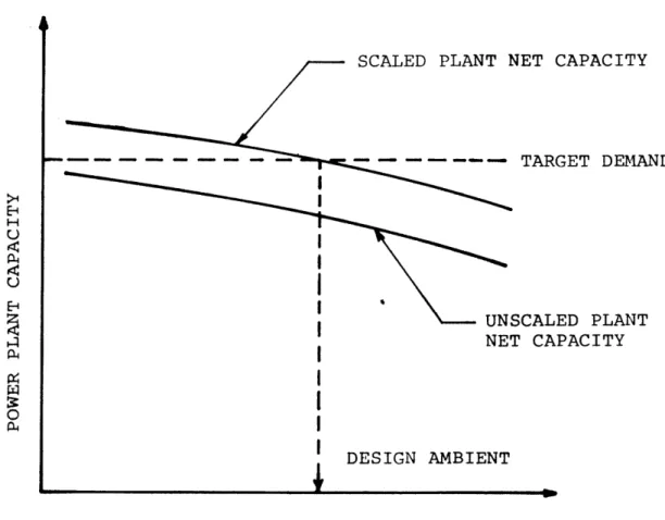
In this study the dry cooling tower system is taken to be an in-direct type with surface condensers and metal-finned-tube heat exchangers.

The computer optimization program does not use pre-designed heat

ex-changer modules. In addition, the piping system design is considered

in detail. Theair flow in the cooling tower is mechanically induced

by fans. The various components of the dry cooling tower system are

shown in Fig. 4.1.

Condensation of the turbine exhaust steam takes place in the

sur-face condenser at the saturated steam temperature corresponding to a

given tbine exhaust prssure. e condceasate is returned to the

TURBINE

PIPING PUMP

FIGURE 4.1 INDIRECT TYPE OF MECHANICAL DRAFT DRY COOLING TOWER SYSTEM DRY TOWER AIR FLOVF XCE MNSER )WATER IT

T is heated to a temperature T2 on leaving the condenser. The

dif-ference between the saturated steam temperature and the hot water tem-perature T is the terminal temperature difference (TTD). The tem-perature difference between T₁ and T₂ is the water range. On

leav-ing the condenser, the hot water is circulated through the pipleav-ing system to the dry cooling towers where heat is rejected to the air from the heat exchangers. The difference between the temperature of hot water entering the dry tower and the temperature of the incoming ambient air

is the initial temperature difference (ITD). After cooling, the water leaving the dry tower is returned to the condenser. Ambient air

enter-ing the dry coolenter-ing tower at a temperature T₁ leaves the tower at a

a a a

temperature T2 . The difference between T2 and T1 is called the

air range. The temperature relationships are illustrated in Fig. 4.2.

4.2 Condenser

The surface condenser in this study is a shell-and-tube heat ex-changer and it is a single pressure design. The circulating water flows

inside the tubes and the turbine exhaust steam is condensed on the outer surface of these tubings. For a thermodynamic equilibrium, the follow-ing equalities must hold:

Qs = UA(LMTD) (4.1)

Q

=

(-

T)

(4.2)

Q* w

Qs Q(4 3)

TTD sat sat mW w 1 1

Tsat= SATURATED STEAM TEMPERATURE AT TURBINE OUTLET

TTD= CONDENSER TERMINAL TEMPERATURE DIFFERENCE ITD= INITIAL TEMPERATURE DIFFERENCE

w

T1₁ = COOL WATER TEMPERATURE

w

T2₂ = HOT WATER TEMPERATURE

a = TEMPERATURE OF AMBIENT AIR ENTERING DRY TOWER

T1

a = TEMPERATURE OF AIR LEAVING DRY TOWER

T2

FIGURE 4.2 TEMPERATURE RELATIONSHIP IN INDIRECT TYPE OF DRY COOLING TOWER SYSTEM

where Qs Qc m w w T2 w T1 U A

= heat rejection rate of the condenser (Btu/hr);

= heat rejection rate to the circulating water (Btu/hr); = condenser circulating water flow rate (lb/hr);

= temperature of hot water leaving the condenser (F); = temperature of cool water entering the condenser (F); = condenser heat transfer coefficient (Btu/hrft2° F); = condenser heat transfer area (ft2);

and

LMTD = log mean temperature difference

w w

T2 - T1 Range

=

~

r'rD+T~-TY =Zn

(Range

+ TTD

TTD TD

Zn(TD+T T T D -T) n/ a n e + )

The overall heat transfer coefficient U based on the ox

face area of condenser tubes is given by

1 1 r r r 1 + °n o o h r.h. k r. o 1 1 a 1 where h = h. = 1 r = 0 r.= 1 k = a (4.4) utside sur-, (4.5)

steam side heat transfer coefficient (Btu/hr-ft2°F);

water side heat transfer coefficient (Btu/hrft2°F);

condenser tube outer radius (ft);

condenser tube inner radius (ft);

conductivity of condenser tube material (Btu/hrft°F).

The water side heat transfer coefficient h. can be calculated using

1

the heat transfer correlation for fully developed turbulent flow. The

h. = 1

0.023 k Re 0.8 Pr 0.4

w w w

d (4.6)

where k = conductivity of water inside condenser tube (Btu/hr-ft°F);

w

Re = water side Reynolds number;

w

Pr = water side Prandtl number;

w

d = tube inner diameter (ft).

The steam side heat transfer coefficient h may be determined by

0

using Nusselt's analysis of condensation on tube banks in the literature

[13,35]. The steam side heat transfer coefficient is given by:

4

h =

0o 0.728 (4.7)

D (Tsv -_s s)

where h = heat transfer coefficient (Btu/hrft2°F);

o

K = thermal conductivity of liquid (Btu/hrft°F);

p = density of liquid (lb/ft3);

Pv = density of vapor (lb/ft3);

g = gravitational force (ft2/hr);

h' = latent heat of condensation (Btu/lb);

fg

1 = viscosity of liquid (lb/hr-ft);

D = tube diameter (ft);

Tv = temperature of saturated vapor (F); sv

T = wall surface temperature (F).

s

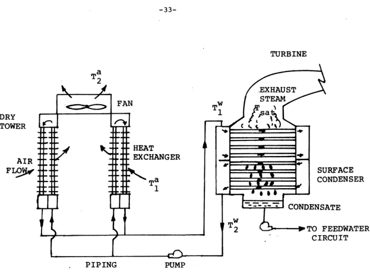
In a large power plant condenser, T ~100°F, (T -T ) 10°F, and

sv sv s

p = 62 lb/ft3 Pv = 0.2 lb/ft3 K = 0.364 Btu/hroft°F h' = 888.8 Btu/lb fg pR,= 1.65 lb/hr-ft

For D = 1 inch, then the steam side heat transfer coefficient is

h = 0.728 (0.364)3 (61.8)2 (4.17 x 108).(888.8)

¼

h = 0.728

0 (1/12) (1.65) (10)

= 1932 Btu/hr-ft2°F .

In Eq. (4.5), with r = 0.5 inches, r = 0.451 inches, k = 65

o 1 a

Btu/hrft°F for admiralty, and the properties of water at 70°F being Pr = 6.82, V = 1.02X 10- 5, K = 0.347 Btu/hrft°F, the overall heat transfer coefficient U is computed for different condenser water velocities. The results are tabulated in Table 4.1.

TABLE 4.1 Condenser Heat Transfer Coeffi-cient vs. Water Velocity

V (ft/sec) h. (Btu/hroft2°F) U (Btu/hr-ft2°F)

1 8 1497.0 842.9 7 1345.0 797.2 6 1189.0 745.0 5 1026.0 683.6 4 860 612.6

In the above calculations, only one horizontal tube is considered. For n tubes, the average steam side heat transfer coefficient should be divided by (n) 4 in Nusselt's correlation in Eq. (4.7) [14,35].

The Heat Exchange Institute [7] has conducted extensive tests for arriving at values of the overall heat transfer coefficient for various tube materials, water velocities, and water temperatures. For example, with the condenser inlet water temperature of 70°F and No. 18 BWG clean admiralty tubes, their experimental data gave the relation between the overall heat transfer coefficient and water velocity as

U = C V0 5 , (4.8)

where U = overall heat transfer coefficient (Btu/hreft2°F); V = water velocity (ft/sec);

C = coefficient = 263 for No. 18 BWG admiralty tubes. u

The results of U from this correlation for various water velocities are calculated and compared to the results obtained by Nusselt's analy-sis in Table 4.2.

TABLE 4.2 Comparison of Condenser Heat Transfer Coeffi-cients Obtained by Nusselt Analysis and Empirical Correlation Given by Heat Exchange Institute

U, Heat Exchange V U, Nusselt's Analysis Institute Test Data (ft/sec) (Btu/hr'ft2°F) (Btu/hr-ft2°F)

8 842.9 743.8

7 797.2 695.8

6 745.0 644.2

5 683.6 588.1

Just based on these first estimations, the Heat Exchange Institute test

data appear to be reasonable.

The water side heat transfer coefficient is a function of the

pro-perties of water and the tube diameter. The thermal resistance of the

tube wall is dependent on the tube inner and outer diameters. For inlet

water temperature other than 70°F and tube wall thickness other than that

of No. 18 BWG, the Heat Exchange Institute provides design correction

factors for Eq. (4.8). Furthermore, a cleanliness factor has to be

allowed for dirty tubes.

Given the values of the condenser water range, the TTD, the water

velocity V, and the heat rejection rate Q , then the total condenser

heat transfer area can be calculated. Mathematically, this is

A = . (4.6)

Range

U n [(TTD+ Range)/TTD]

Also, from the heat rejection rate and the water range, the water flow

rate can be calculated; that is,

=

m - (4.7)

Ran9_e

by taking the specific heat of water to be 1 Btu/lb°F.

By applying the mass conservation principle to the water flow rate,

we have m = PVAH (4.8) or (4.9) m .A = -E. P

where p = density of water (lb/ft 3

) at the mean temperature of T

w

and T2 ;

2~~~~~~~~

A_H = total hydraulic area (ft2).

Given the inner diameter of the condenser tubes, then the total

number of tubes is

4A_H

nT 2 (4.10)

7TD.

where D. = tube inner diameter (ft).

1

Finally, from the total heat transfer area, the outer diameter of

the tubes and the number of tubes, the condenser tube length can be

determined from the following equation:

= A AT

nTrD (ft) (4.11)

~T = n 7TD

T o

where D = tube outer diameter (ft).

0o

In designing the condenser, the Heat Exchange Institute [7]

recom-mends a minimum design TTD of 5F to avoid unpredictable condenser

per-formance at design TTD's below this limit.

The relation between the heat rejection rate and the TTD can be

calculated from Eqs. (4.6) and (4.7). For a fixed condenser design,

the water flow rate m , the heat transfer area A , and the overall heat

transfer coefficient U are constant. By combining Eqs. (4.6) and (4.7)

we get

TTD Q/m

£n

(TDTTD

/

A =

or * v An TTD + Q/m = A constant TTD m Therefore, 1 + Q ... = constant (m)(TTD) or = constant (m)(TTD) Finally, we get Q = constant* TTD . (4.12)

The maximum condenser tube length is about 50 ft. Thus, two passes are

needed if the tube were longer than about 50 ft.

Due to corrosion and erosion problems, the condenser water velocity

is constrained to a maximum of 7 ft/sec [12].

As can be seen in Eqs. (4.5) and (4.6), with the heat rejection

rate, the TTD, and the range being fixed, the heat transfer area is

inversely proportional to the square root of the water velocity; that

is,

A 1

This means a higher water velocity gives a smaller condenser. However,

the higher the water velocity, the larger the pumping power requirement

(Appendix I gives the pressure drop relationships). Hence there is a

trade-off between the capital cost of the condenser and the pumping

power ost.

cost, tube cost, and field erection cost. A detailed cost algorithm

of the condenser is given in Appendix II.

4.3 Dry Towers

In general, mechanical draft dry cooling towers can be circular

or rectilinear in shape. Rectilinear towers often have the heat

ex-changer bundles supported horizontally about 50 ft above the ground.

In circular towers the heat exchanger bundles are normally vertically

arranged around the base of the tower and, therefore, they are rather

self-supporting and require less structural support than the rectilinear

towers. The methodology of heat exchanger design follows Andeen et al.

[1,2,3]. Assuming a cross-flow heat exchanger with the water side

un-mixed, we have the following two cases:

Case I: C /C < 1 ; that is, C = C , C = Clarge

w'a w small a large

The effectiveness is given by

C = 1 - exp - - (1 - e TU) (4.13)

a

where NTU = UA/C smal. This gives

/small NTU = -n 1 + a n 1 -- - (4.14) C C' w a By definition, C (T -T ) £ - c c2 cl (4.15) C l(TH- T ) small H1 cl

where the subscripts H = hot fluid; C= cold fluid;

1 = in; 2 = out. Here, CH_H = C _w = Cs _small , and

AT

W

C= wTD (4.16)

ITD

C

/

c

AT

NTU

=-[i

+

a

1ID)]

C

(4.17)

Case II: Cw/C > 1; that is, Clarge = Cw, Csmall a

w a lre w sal a Then, C -NTU C /C\ s = 1 - exp -w( - e , (4.18) which gives C C C NTU = - C + - ) (4.19) a W Here, CH = C =C l a r ge , and H W large C AT = _{C W (4.20)} CITD a C C

C

AT NTU = n

1

+ a n 1

I

. (4.21) C

~

~

CC fTD a C W a

For a fixed dry cooling tower design in either Case I or Case II, with the air flow rate and the water flow rate constant, the

AT

£ = constant = - in Case I

ITD

or C AT

£ = constant = in Case II.

C ITD

a

Thus, AT iITD = constant, and since m is constant, we have

w m AT w w = constant ITD or = constant ITD or Q = constant* ITD . (4.22)

To evaluate the heat rejection capability of a mechanical draft dry

cooling tower at off-design conditions, the following equations can be

employed: QD_{D ' (4.23)} ITD ITDD or ITD (4.24) QD ITDD '

where Q = heat rejection rate at off-design (Btu/hr);

D = design heat rejection rate (Btu/hr);

ITD = initial temperature difference at off-design (F);

ITDD = design initial temperature difference (F).

The mass velocity of air flow is given by

m

G = A (lb/hrft2)

A

where ma = mass flow rate of air (lb/hr);

A = free flow area of heat exchanger (ft2

But A = AF , (4.25)

where 0 = ratio of free flow area to frontal area; AF = frontal area of heat exchanger (ft2). It follows that the air-side Reynolds number is

GD

Re = e (4.26)

a

~a where G = mass velocity;

D = equivalent diameter; e

Ua = viscosity of air.

If the Colburn factor and friction factor as a function of the air-side Reynolds number are known, for example given in Kays and London [9], then the air-side heat transfer coefficient h can be obtained from the

fol-o lowing relation: h 0 213 St Pr = o pr2 3 , (4.27) a a so that

_~~so

_that

_~St

_{Pr GC}

h a (4.28)

pr2/3

Andeen et at. used the following equation to calculate the fin efficiency. Andeen [34] obtained this equation from a Dynatech report.

Fin efficiency nf = (4.29)

Eh (D- OD)2 1 +

24 KT

where K = thermal conductivity of fin (Btu/hr-ft°F); D = fin diameter (inch);

OD = tube outer diameter (inch);

E = (D/OD + 4/3)/7 ;

T = fin thickness (inch).

The overall surface efficiency n is given as s

A (1 -pT

ni = (4.30)f(Af

T

where Af = fin area;

A_T = total surface area. T

The water-side heat transfer coefficient h. is determined by 1

the following equations:

h.D Nu. 1 = 0.023 Re0'8 Pr0" (4.31) 1 K w w or 0.023K Re° 8 Pr 0 4 h. =

~w

w h. _{1 D}D (4.32)

where Nu. = Nusselt number; 1

D = tube inner diameter;

K = thermal conductivity of water in tube; Re = water-side Reynolds number;

w

Pr = water-side Prandtl number.

w

The overall heat transfer coefficient U is given by

1 1 + 1 (4.33)

U (ns 1 -- )h

ATE I Using the NTU relationship

UA a CNTU

= (4.34)

small where A is the air-side surface area, then

a

NTU Csma1

A =

-a U

The volume of the heat exchanger is given by A

-a

V= _a a , (4.35)

a

where a is the surface area per unit volume of heat exchanger. Finally, the depth of the heat exchanger dT can be calculated

by the following relationships:

V = AF dT (4.36)

a

or V

d_T a (4.37)

T AF

After determining the dimensions of the heat exchanger for a given heat transfer surface, then the total installed cost of the heat exchanger can be calculated.

In this study each circular tower is divided into four quadrants; a quadrant can be shut down and isolated from the main circulation pipes by closing the control valve. All quadrants have the same number of heat exchanger bundles (schematic sketch given in Fig. 4.4).

A heat transfer bundle is composed of heat transfer surfaces (finned tubes), headers, bundle frame, and cross supports. The cost of the heat transfer surface is the sum of tubing cost, finning cost, surface coat-ing cost, and tube spacer cost. The total installed cost of a bundle

consists of the costs of the heat transfer surface, header, framing, and assembly. A detailed cost algorithm for the heat exchanger is given in Appendix II.

4.4 Piping System

The piping system circulates the cooling water between the heat exchanger bundles and the condenser. It consists of the main circula-tion lines and tower distribucircula-tion pipes. The piping model is adopted from Ref. 12. Figures 4.3 and 4.4 illustrate the piping layouts. A reasonable distance of 500 ft between the condenser and the cooling tower is assumed. The center-to-center distance between the circular towers is taken to be one and a half times the tower diameter and this

is believed to be sufficient for air circulation between towers [12]. The piping material is welded carbon steel with a design pressure of 125 psig. Pipe diameters are available from 12 to 144 inches with size increments of 6 inches. Due to corrosion and erosion problems, the maximum allowable piping water velocity is 20 ft/sec [12].

For a given water flow rate, a higher water velocity results in a smaller pipe diameter but it increases the hydraulic pressure drop or pumping power requirement. Therefore, there is a trade-off between the piping capital cost and the cost of pumping power.

The piping water velocity optimization is given in Appendix III. For pipes installed either below or above ground level, the optimum design water velocities for large flow rates from 5000 to 500,000 gpm

-50-2, ~2. 5D t

500 f'r 1)-.I

-.---

DRY 1TOERS

PIPING

SINGLE TOWER GROUP

4--

-

2.5 D

D al,

500 FT

T

2.5D DRY ITOWERS

DaUBLE TOWER GROUP

FIGURE 4.3 DRY COLING TOWER SYSTEM PIPING IAYOUT

T

2.5D

C IRCULATION WER DISTRIBUTION PIPING HEAT EXCHANGER BUNDLES QUADRANT HEADER PIPING I

TOWER DISTRIBUTION PIPING

FIGURE 4.4 DRY TOWER PIPING AIR FLOW WATER FLOW % I

are in the vicinity of about 12.5 ft/sec.

In addition to pipes, the piping system is also composed of neces-sary pipe fittings such as reducers, elbows, tees, valves, and flanges. A detailed cost algorithm for pipes and pipe fittings is given in Appen-dix II.

4.5 Pumping System

The pumping system provides the necessary pumping head to overcome the hydraulic pressure drops in the cooling system. It consists of cir-culating pumps, pump structure, motors, and electrical equipment. The total pumping power requirement is governed by the water flow rate and total pressure drop of the cooling system. For the dry cooling tower system the total pressure drop is the sum of the pressure drops in the condenser, piping, and heat exchanger. The pressure loss in pipe fit-tings is believed to be 30-45 percent of the pressure drop in the pipes

[8]. A value of 45% is used in this study.

The overall pumping efficiency (pump and motors) is estimated to be about 87.6% [20]. The pump brake horsepower BHP is given by

P AP_T(pQ)

BHP _p

_550nh

550 (4.38)

p where APT = total pressure drop (ft H20);

Q = water flow rate (ft3/sec); rp = pumping system efficiency; p = density of water (lb/ft3).

CHAPTER 5:

OPTIMIZATION OF DRY COOLING TOWER SYSTEMS AND RESULTS

The computer optimization program of the dry cooling tower systems

in this study follows Andeen and Glicksman 1,2,3]. The program does

not use pre-designed heat exchanger modules; rather, it optimizes the

dimensions, air loading, water loading, etc., for the heat exchanger.

5.1 Introduction

In the present model the six design variables used in the program

are the ambient dry bulb temperature, the initial temperature

differ-ence (ITD), the water range, the water-to-air heat capacity ratio, the

heat exchanger air-side frontal area, and the width-to-length ratio of

the heat exchanger.

The design dry bulb temperature is the reference temperature at

which the power plant is scaled to produce a given net electrical

out-put. At ambient temperatures higher than this design temperature the

turbine heat rate increases and, therefore, the generating capability

of the power plant decreases.

The design initial temperature difference (ITD) defines the size

of the dry cooling tower. Generally, the higher the ITD the smaller

the dry cooling tower. However, a high ITD often results in a larger

penalty cost.

surface condenser. As discussed in Chapter 4, the mathematical rela-tionship of heat transfer in the condenser is given by

*

UA Range

Qc = UA

c

=

Zn [(Range + TTD)/TTD]

Here, range is the water range. Therefore, for a given heat rejection rate Q , a given U, and a given TTD, the heat transfer area A is a function of the water range only. That is,

Qc

A= = f(range)

Range

Zn [(TTD+ Range)/TTD]

Moreover, the water range also influences the piping system design. The relationship between the heat rejection rate, the water flow rate, and the water range is given by

Qc = (mw )(Range)(Cw) , (5.1)

where Qc = condenser heat rejection rate (Btu/hr); m = mass flow rate of water (lb/hr);

w

Range = water range (F);

Cw = specific heat of water - 1 Btu/lb°F.

For a given heat rejection rate, the higher the range, the smaller the water flow rate. However, for a given design water velocity, a smaller water flow rate requires a smaller pipe diameter.

The capacity ratio is defined as the ratio of the heat capacity of water to the heat capacity of air where heat capacity of a fluid is the

product of the mass flow rate and specific heat of the fluid. For a given water flow rate, the capacity ratio determines the air flow rate for the heat exchanger.

Finally, the frontal area and the width-to-length ratio are used in calculating the dimensions of the heat exchanger. With a given vol-ume of a heat exchanger, increasing the frontal area tends to reduce the depth of the heat exchanger. On the other hand, given the frontal area, a higher width-to-length ratio shortens the heat exchanger tube

length. The dimensions of the heat exchanger affect both the cooling tower arrangement and the piping design.

5.2 Dry Cooling Tower Optimization Procedure

With a given heat transfer surface, a given turbine heat rate characteristic, a specified net capacity, a given set of economic parameters, a given set of meteorological data (for dry tower, only the dry bulb temperature distribution is needed), and the six design variables discussed in the previous section, optimization can then be performed. The optimization involves a selection of an optimum from a set of optima. The procedures are as follows:

(1) Select a design dry bulb temperature.

(2) Select a design initial temperature difference (ITD).

(3) Find the combination of the water range, capacity ratio, heat exchanger frontal area, and width-to-length ratio that gives the minimum power generation cost for the power plant with the dry

cooling tower system. Here, scaling of the power plant is

per-formed so that the net capacity is equal to the target demand by

assuming the design ambient temperature to be the temperature

throughout the year.

(4) Evaluate the performance of the power plant with the dry cooling

tower system over an annual cycle and determine the capacity and

energy penalties. Obtain the power production cost.

(5) Repeat the procedures (2)-(4) with a new design ITD.

(6) Plot the power production cost vs. the design ITD and obtain the

global optimum.

(7) Repeat the procedures ()-(6) with a new design dry bulb

tempera-ture.

(8) Compare the optima obtained for the selected design dry bulb

tem-peratures and pick the minimum.

The optimum combination of range, capacity ratio, frontal area,

and width-to-length ratio is obtained by the minimization method

devel-oped by Andeen and Glicksman [1,2,3]. The minimization technique

in-volves a double-shotgun-and-search method. To explain how the method

is used, let us consider a simplified case. Assume cost is a function

of two independent variables; then it is pictured as a surface in

two-dimensional space, as shown in Fig. 5.la. To obtain a starting point

in the proximity of the optimum design point, first, the coarse

shot-gun is used to evaluate the cost of a random initial point (point 1,