HAL Id: halshs-01168660
https://halshs.archives-ouvertes.fr/halshs-01168660
Preprint submitted on 26 Jun 2015
HAL is a multi-disciplinary open access archive for the deposit and dissemination of sci-entific research documents, whether they are pub-lished or not. The documents may come from teaching and research institutions in France or abroad, or from public or private research centers.
L’archive ouverte pluridisciplinaire HAL, est destinée au dépôt et à la diffusion de documents scientifiques de niveau recherche, publiés ou non, émanant des établissements d’enseignement et de recherche français ou étrangers, des laboratoires publics ou privés.
Wealth Effects on Consumption across the Wealth
Distribution: Empirical Evidence
Luc Arrondel, Pierre Lamarche, Frédérique Savignac
To cite this version:
Luc Arrondel, Pierre Lamarche, Frédérique Savignac. Wealth Effects on Consumption across the Wealth Distribution: Empirical Evidence. 2015. �halshs-01168660�
WORKING PAPER N° 2015 – 17
Wealth Effects on Consumption across the Wealth Distribution:
Empirical Evidence
Luc Arrondel Pierre Lamarche Frédérique Savignac
JEL Codes: D12, E21, C21
Keywords: Consumption, Marginal propensity to consume out of wealth, Policy distributive effects, Household survey
P
ARIS-
JOURDANS
CIENCESE
CONOMIQUES48, BD JOURDAN – E.N.S. – 75014 PARIS TÉL. : 33(0) 1 43 13 63 00 – FAX : 33 (0) 1 43 13 63 10
Wealth Effects on Consumption across the Wealth Distribution:
Empirical Evidence
*Luc Arrondel**, Pierre Lamarche***, Frédérique Savignac****
June 2015 Abstract
This paper studies the heterogeneity of the marginal propensity to consume out of wealth using French household surveys. We find decreasing marginal propensity to consume out of wealth across the wealth distribution for all net wealth components. The marginal propensity to consume out of financial assets tends to be higher compared with the effect of housing assets, except in the top of the wealth distribution. Consumption is less sensitive to the value of the main residence than to other housing assets. We also investigate the heterogeneity arising from indebtedness and from the role of housing assets as collateral.
Classification: D12, E21, C21
Key words: Consumption, Marginal propensity to consume out of wealth, Policy distributive effects, Household survey
*We would like to thank Henri Fraisse, Arthur Kennickell, Erwan Gautier, Claire Labonne, Julien Matheron, Ernesto Villanueva, Jirka Slacalek for helpful discussions and suggestions as well as participants to the Household Finance and Consumption Research Workshop (March 2014).
This paper presents the views of the authors and should not be interpreted as reflecting the views of the ECB or of Banque de France.
** CNRS-PSE , Banque de France. arrondel@pse.ens.fr *** European Central Bank. Pierre.Lamarche@ecb.europa.eu
Non-technical summary
The effect of wealth on households’ behavior is a crucial issue for the monetary policy transmission to the real economy. Therefore, the link between wealth and consumption is widely discussed in the literature. According to the life cycle theory, wealth accumulation is used to smooth consumption over the life-cycle. As a result, any unexpected changes in wealth resulting from unanticipated developments in stock or housing prices may lead households to adapt their consumption. An extensive literature estimates the wealth effect on consumption using aggregate data. However the overall consumption may result from the aggregation of consumption behaviors that differ across sub-populations, which cannot be taken into account in macro-based estimates. In particular, the heterogeneity in the composition of the population (renters versus homeowners, stockholders, etc.) together with the wealth concentration in the top of the wealth distribution is likely to induce differences in consumption behaviors across households.
This paper aims at providing new insights on the heterogeneity of the wealth effects on consumption. It estimates the marginal propensity to consume out of wealth (MPC) across the whole wealth distribution and accounts for differences in the wealth composition at the household level using the French Wealth Survey1 (INSEE) combined with the Household
Budget Survey (INSEE-EUROSTAT).
We address the following questions: Is the marginal propensity to consume out of wealth decreasing with wealth? By how much does it vary across the wealth distribution? Is the MPC pattern similar for housing and financial assets? Which wealth effects (housing or financial wealth) does dominate, depending on the household position in the wealth distribution? How does the household’s indebtedness (level and type of collateral) affect the MPC?
Existing macro-based MPC estimates for France (see Slacalek (2009) for instance) found small but significant wealth effects on consumption in France, with estimated marginal propensity to consume out of wealth (MPC) ranging from 0.8 of a cent to 1 cent on annual consumption for every 1 euro increase (compared with MPC estimated around 5 cents for the U.S or the U.K). Our micro-based results confirm this limited wealth effect on consumption. More interestingly, when allowing for heterogeneous wealth effects across the wealth distribution, we obtain a decreasing marginal propensity to consume out of wealth along the
wealth distribution. The marginal propensity to consume out of financial wealth decreases from 11.5 cents in the bottom of the wealth distribution to a non-significant effect in the top of the distribution. The marginal propensity to consume out of housing wealth decreases from 1.1 cent in the bottom of the wealth distribution to 0.7 cent in the top of the distribution. For most households, the marginal propensity to consume out of financial assets tends to be higher compared with the marginal propensity to consume out of housing assets, except in the top of the wealth distribution, where the effect is the other way around.
This paper also contributes to the debate on whether there is a direct wealth effect on consumption or whether the correlation between wealth and consumption partly reflects a confidence channel. Our MPC estimates are obtained by controlling for household subjective income expectations and our results support the views of the existence of a confidence effect in addition to the direct wealth effect on consumption.
We also investigate the collateral effect of housing assets in France and we find larger MPC for households that have contracted mortgages, everything else being equal. Such differences in the marginal propensity to consume out of wealth are then consistent with a possible collateral effect which would lead the consumption of “mortgage households” to be more sensitive to housing wealth. Given the institutional features of the mortgage market in France, such a result could also reflect a selection effect in the bank lending supply.
1. Introduction
Whether or not there is a consumption wealth channel at play is a crucial policy issue, especially for the monetary policy transmission to consumer behaviors (see for instance, Ludvigson et al., 2002); this is why a large empirical macroeconomic literature (see among others Muellbauer, 2010; Carroll et al., 2011 or Aron et al., 2012) aims at evaluating the macroeconomic impact of wealth on consumption. However, those macro-based estimates are not able to account for heterogeneities in households’ behavior. Indeed, the overall consumption may result from the aggregation of consumption behaviors that differ across populations. From a theoretical point of view, Carroll and Kimball (1996) show that uncertainty over wealth and income may lead the marginal propensity to consume out of wealth to decline as wealth or income increase. Formerly, they show that when households have precautionary saving motives, in presence of income uncertainty, the consumption function is concave regarding wealth2. The intuition behind the decreasing marginal propensity to consume out of wealth is that wealthy households save for precautionary motives proportionally less than none-wealthy ones. Under uncertainty, King (1994) shows that credit constraints also induce higher marginal propensity to consume out of wealth. Liquidity constrained households cannot adopt their optimal consumption and their consumption is more sensitive to wealth (Blinder, 1976). Such heterogeneity in the marginal propensity to consume out of wealth would impact the transmission of prices to consumption and is therefore of primary interest for policy design.
This paper estimates the marginal propensity to consume out of wealth (MPC) across the whole wealth distribution and accounting for differences in the wealth composition at the household level. Existing empirical evidence of the heterogeneity in the marginal propensity
2 Carroll and Kimball (1996) show that uncertainty induces a concave consumption function for a very broad class of utility
to consume out of wealth depending on the wealth level are scarce. Mian et al. (2013) addresse this question relying on geographical prices variations across the U. S. They show that ZIP codes with poorer and more levered households have a significantly higher marginal propensity to consume out of housing wealth. However, given the data they use, the effect of two major features of the household wealth distribution cannot be investigated. First, wealth distribution is highly skewed to the right (e.g. Campbell, 2006) meaning that the overall consumption-wealth relationship may be driven only by part of the population in the top of the wealth distribution. Second, wealth composition, especially the relative shares of financial and housing assets in household wealth, varies along the wealth distribution (see Arrondel et al., 2014 for euro area countries), leading to differences in wealth shocks exposure along the wealth distribution. Some other papers account for possible differentiated marginal propensities to consume out of wealth depending on the level of wealth relying on wealth survey (Bover, 2005; Bostic et al., 2009; Grant and Peltonen, 2008; Paiella, 2007 or Sierminska and Takhtamanova, 2007)3. However, they do not investigate in a more detailed
way this heterogeneity across the wealth distribution and depending on the wealth composition.4
For such a purpose, household level data covering both wealth and consumption distributions are needed (Poterba, 2000; Paiella, 2009). Our paper uses the 2010 French Wealth Survey which is specifically designed to measure the wealth distribution in France5.
This survey provides detailed information on assets composition, debt, income, socio-demographics and expectations. It also includes some questions about consumption for a
3Parker (1999), Bover (2005) and Arrondel et al. (2014a) find evidences of decreasing marginal propensity to consume out
of wealth using respectively U.S., Spanish and French data while Grant and Peltonen (2008) do not find such significant differences across wealth levels for Italy.
4Another strand of the empirical literature aims at identifying the wealth effects on consumption controlling for heterogeneity
in households’ behaviors relying on prices dynamics (Attanasio et al. 2009, Browning et al., 2013; Campbell and Cocco 2007; Disney et al. 2010). These papers studies the MPC heterogeneity across age or homeownership status, but given the empirical stategy used (impact of prices dynamics), they cannot examine the MPC heterogeneity arising from net wealth composition and wealth inequality.
5The French wealth survey is conducted by the National Statistical Institute (INSEE) and is part of the Household Finance
subsample of households so that we can use a consumption survey, the Household Budget Survey (INSEE-EUROSTAT), to measure consumption at the household level, following the statistical matching methodology proposed by Browning et al. (2003). We are thus able to properly account for both the wealth and the consumption distributions. We then exploit the cross-sectional differences in consumption behaviours and wealth (level and composition) across households to estimate the marginal propensity to consume out of wealth (see Parker, 1999; Bover, 2005 or Paiella, 2007 for similar approaches). Our empirical model is based on a simple consumption function: the consumption-to-income ratio is regressed on the wealth-to-income ratio and on several control variables accounting for the household life-cycle position, preferences, risk exposure, and income expectations. We allow heterogeneous wealth effects across the wealth distribution and across net wealth components. We extend the empirical literature on the heterogeneity of the wealth effect on consumption in the following ways:
First, we find a decreasing marginal propensity to consume out of financial and housing wealth across the wealth distribution. The marginal propensity to consume out of financial wealth decreases from 11.5 cents in the bottom of the wealth distribution to a non-significant effect in the top of the distribution. The marginal propensity to consume out of housing wealth decreases from 1.1 cent in the bottom of the wealth distribution to 0.7 cent in the top of the distribution. When ignoring this heterogeneity across the wealth distribution, our micro-based estimates are in line with the macro-based ones6: the micro-based estimated
marginal propensity to consume out of wealth is about 0.006 for the whole population, meaning that one additional euro of net wealth would be associated with 0.6 cent of euro of additional annual consumption, and macro-based estimates range from 0.8 of a cent to 1 cent on annual consumption for every 1 euro increase (Chauvin and Damette, 2010, Slacalek, 2009). Our results confirm then the small but significant wealth effects on consumption in
6In the case of France, the existing MPC estimates were only macro-based ones. This paper is then the first one providing
France (compared with MPC estimated around 5 cents for the U.S or the U.K, see Slacalek (2009) for instance); but most importantly, we highlight the heterogeneity in the marginal propensity to consume out of wealth. This heterogeneity is driven both by differences in the wealth composition and in the wealth level. Then, we compute the average consumption elasticity to wealth in each wealth group in order to investigate the implications for aggregate consumption. While the estimated MPC is decreasing with wealth, it is not the case for the consumption elasticity to wealth because the wealth concentration in the top of the distribution counterbalances the effect of the decreasing marginal propensity to consume out of wealth. In other words, average wealth increases more than average consumption across the wealth groups (reflecting the skewness of the wealth distribution), so that even with decreasing MPC, a one percent of additional wealth has a greater effect on consumption in the top of the wealth distribution.
Second, we examine the role of leverage and liquidity constraints. We compare the MPC for subpopulations facing heavy versus light debt pressures. Our results suggest that consumption for households facing heavy debt pressures is more sensitive to financial wealth except in the bottom of the net wealth distribution, where highly indebted household would rather reimburse their debt than consume an additional euro of financial wealth.
Third, we investigate another possible source for MPC heterogeneity, the collateral channel effect of housing wealth: higher housing wealth, everything else being equal, may relax financing constraints faced by households who have contracted loans guaranteed by the value of their housing assets (mortgages). We find larger values of MPC out of housing wealth for households that have loans with real estate collateral. We discuss the institutional features of the mortgage market in France and argue that such a result is more likely to reflect a selection effect in the bank lending supply policy rather than additional borrowing capacity for consumption purposes.
Fourth, this paper also contributes to the literature on whether there is a direct wealth effect on consumption or whether the correlation between wealth and consumption partly reflects a confidence channel (Poterba, 2000; Fenz and Fessler, 2008). We follow Disney et al. (2010) and consider a proxy for subjective expectations on future (5 years ahead) total income of the household as additional control variable7. We find that the probability to expect
an increase in the household total income has a positive significant effect on the consumption-to-income ratio. However, in our case, the introduction of this variable does not affect the estimated marginal propensity to consume out of wealth. Our results support the views of the existence of a direct wealth effect on consumption, in addition to the confidence channel.
This paper is organized as follows. Section 2 describes our data and imputation strategy. In Section 3 we present our empirical approach and baseline regression. Our main results on the heterogeneity of the marginal propensity to consume out of wealth are discussed in Section 4. Section 5 investigates the role of debt pressure and the existence of a collateral channel. Section 6 concludes.
2. Wealth and consumption at the household level 2.1. Data sources
Our empirical analysis is based on the French Wealth Survey (Enquête Patrimoine - INSEE). We also use the Household Budget Survey 2006 (HBS, INSEE) to impute consumption at the household level in the French Wealth Survey, following the statistical matching approach proposed by Browning et al. (2003).
The French Wealth survey (FWS) is designed to measure household wealth distribution. This survey provides detailed information at the household level on housing wealth (household main residence, other residences), financial wealth, business assets, debts
7In the French Wealth Survey, subjective expectations are collected for a subsample of households which is not the same as
(mortgages and other debts), consumption and socio demographic variables (household composition, employment status, etc.). We use the 2009/2010 wave which was conducted between October 2009 and February 2010. It is a cross-section sample of 15,006 households. The sampling design ensures representativeness of the population and accounts for the wealth concentration (oversampling of the top of the distribution), see HFCN (2013) for the detailed methodology of the survey.
The measure of consumption is a crucial issue. The best household level information about consumption distribution is provided by the Household Budget Surveys (HBS). These surveys collect item expenditures by asking households to fill in a very detailed diary. Unfortunately the HBS cannot be merged with the FWS for two reasons. First both datasets are anonymised and second they do not cover the same sample of households. We nevertheless take advantage of the French 2006 Household Budget Survey8 to impute
consumption in the French wealth survey.
2.2. Consumption measure
We follow the methodology proposed by Browning et al. (2003) and estimate an auxiliary model on the HBS to predict non-durable consumption in the FWS. For that purpose, a set of questions about consumption have been included in the French Wealth Survey. These questions deal with well-defined and limited parts of the household’s expenditures (food consumption at home, food consumption outside the home and utilities). These consumption items are also covered by the HBS. First, using the HBS, non-durable consumption is regressed on the selected expenditure items (food consumption at home, food consumption outside the home and utilities) and on a set of qualitative indicators reflecting
regular expenses for 8 other items (clothing, public transport, cultural goods, etc.). 9 Then, the
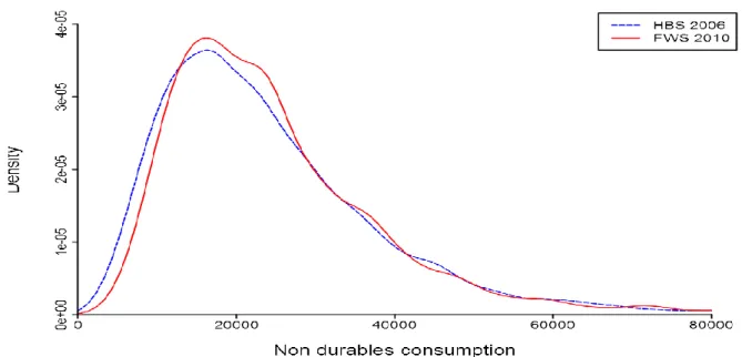
coefficients from this auxiliary regression estimated on the HBS are used to impute the non-durable consumption in the Wealth Survey. The imputation strategy is detailed in Appendix A. Various tests have been conducted to evaluate the imputation procedure (see Appendix A). In particular, the distributions of the imputed consumption variable in the FWS on the one hand and the original variable measured in the HBS on the other hand are very close (see Fig. 1). Moreover, our consumption measure in the Wealth Survey covers 90% of the National Accounts aggregate. 10
[INSERT FIG. 1]
2.3. Consumption and wealth distributions
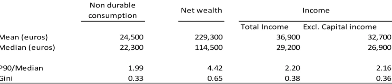
Table 1 reports summary statistic for consumption, wealth and income distribution based on our data11. They are in line with well-known facts about the distributions of consumption,
wealth and income.
[INSERT TABLE 1]
First, consumption is less unequally distributed than income (e.g. Blundell et al., 2008). In France, according to the French Wealth survey, the Gini coefficient for total gross income is about 0.38 (and about 0.36 when excluding income from housing and financial assets). For non-durable consumption, the Gini coefficient is slightly lower (0.33). The fact that durable consumption is less unequally distributed than income is also supported by the ratio of the top ten to the median value: top ten durable consumption is less than 2 times more than the median, while this ratio is around 2.2 for income. Second, wealth is far more unequally distributed than income (e.g. Davies and Shorrocks, 1999). For France, the Gini coefficient of
9 We choose to consider only the available information on the consumption composition in our imputation equation. We do not introduce income or other demographic variables in order to avoid “mechanical” correlation between consumption, income and wealth when estimating the marginal propensity to consume out of wealth.
10 Considering harmonized definitions in both sources.
11 Given the sampling design of the survey, we use final weights to compute our descriptive statistics in order to ensure the representativeness of the figures.
net wealth is about 0.65 and the top ten net wealth is more than 4.4 times the median net wealth. Indeed, household wealth (gross and net values) increases dramatically across the wealth distribution, especially above the median value (Table 2, columns 1 and 2).
[INSERT TABLE 2]
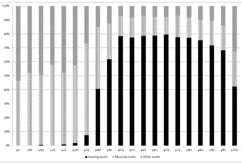
Such a pattern partly reflects the homeownership rate in France (55%) and the key role played by housing assets in the wealth distribution. Indeed, the asset composition varies also a lot across the wealth distribution (Fig. 2). Below the 30th gross wealth percentile, household hold only financial assets (mainly deposits) and other wealth (durable goods and businesses for some of them). Then, the share of housing wealth increases sharply. It reaches about 70% of total assets in the p50-p90 gross wealth percentiles. In the top of the distribution, the weight of housing assets decreases, and its composition changes: the share of the main residence decreases while the share of other housing assets increases. In the top 1%, households hold diversified portfolios where financial assets and other assets have more weight than housing wealth.12 The composition of their assets is also very specific; in particular business assets
play a crucial role in explaining their total wealth. [INSERT FIG. 2]
Concerning debts, one also observes differences across the wealth distribution (Table 2, last column). In the first gross wealth quintile, debt represents about 15% of the value of total assets and the average net wealth is negative. This ratio reaches 16% in the p50-p70 interval and decreases above this threshold. This pattern reflects the fact that most of households are indebted to buy their main residence.
The concentration of wealth combined with the heterogeneity in its composition and the crucial role of debt for some households are then likely to induce differences in the marginal propensity to consumption out of wealth across the wealth distribution.
12 Given the oversampling of wealthy people in the French wealth survey, we are able to provide representative figures for the top 1%.
2.4. Estimation sample and definitions Sample selection
The consumption questions are asked to a (representative) sub-sample of 4,519 households (among the 15,006 households in the full sample). In order to estimate the marginal propensity to consume out of wealth, we exclude households with very specific wealth, income or consumption figures: households with very high values of gross wealth (above 5 million Euros), very low annual income (below 2,000 Euros) or extremes values in the consumption-to-income ratio are then excluded. We also restrict the analysis to households where the reference person is aged between 25 and 65 in order to focus on household engaged in the working life and to avoid survival bias in old ages. In the end, our final estimation sample consists of 3,454 households after cleaning. The composition of the econometric sample is very similar to the full sample with slightly lower mean wealth values (see Table C1 in Appendix C).
Net wealth components
In order to account for the heterogeneity in the wealth composition, we split total wealth into the following components:
- Housing wealth includes two components: the household main residence and other real estate property (holiday homes, rental homes, excluding real estate property held for business purposes). The literature points out that housing wealth has an ambiguous impact on consumption (see for instance Cooper, 2013). On the one hand, housing satisfies consumption needs and its cost increases with housing prices for all households (renters and homeowners) who may have to reduce their non-housing expenditure (negative wealth effect)13. On the other hand, it provides also capital
gains/losses for homeowners who may adapt their consumption plans to these (unrealized or realized) housing gains/losses. The role played by the household main residence is then likely to be specific as it covers both consumption needs and investment motives, while the other real estate properties are more likely to reflect investment decisions.
- Financial wealth includes all financial assets held by the household (deposits, mutual funds, shares, voluntary private pensions, whole life insurance and other financial assets) but excludes business assets;
- Other wealth includes assets held for business purposes (land, farms, office space rented out to businesses, etc.) and all other remaining assets (vehicles, valuables, etc.). For each category of assets, we consider the net values, i.e. the gross value of the considered assets less the remaining principal balance of loans contracted for buying these assets, using the survey information on the main purpose of each contracted loans (see the detailed definition of the variables in the appendix B).
Subjective expectations about income
The FWS provides useful information on subjective expectations of the reference person concerning the expected evolution of the household total income. We construct a dummy variable reflecting that the household is optimistic about the future household total income (i.e. expects a positive average income growth rate 5 years ahead). Such a variable allow disentangling direct wealth effect from a confidence effect14 and has been previously
considered by Disney et al. (2010). In the FWS, subjective expectations are collected only for a subsample of households which is not the same as our estimation sample. We then use an in-sample imputation to construct our proxy. We first estimate the linear probability for a
14 Attanasio et al. (2009) and Carroll et al. (2011) argue that the correlation between consumption and wealth may be
spurious due to omitted common determinants of asset values and consumption such as households’ expectations concerning future productivity growth.
household to expect a positive evolution of the household income within 5 years depending on the detailed household composition, on demographic variables related to the reference person as well as on some information about the parents of the reference person. These variables aim at accounting for the household permanent income and for the heterogeneity in expectations formation. The estimation results (see Table B2 in the Appendix B) show that they are highly correlated with our indicator of income expectations. We then use this estimated model to impute a similar qualitative indicator of optimism in our main estimation sample. The percentage of predicted optimistic households in our estimation sample is very close to the observed one in the initial subsample. The imputation strategy and the results are detailed in the Appendix B.
3. Empirical analysis: baseline model
In order to estimate the marginal propensity to consume out of wealth at the household level and using cross-sectional information, we follow the empirical approach used by Paiella (2007). We consider a simple consumption function based on the life cycle model where individuals use wealth accumulation to smooth consumption over their life cycle. In this framework, current consumption is proportional to total wealth (i.e. the sum of real non-human wealth and real non-human wealth, the latter being defined as the present value of expected future income, see Deaton, 1992) and the the link between consumption, income and net wealth could be described as:
(1)
where Cht and Yht stand for respectively the consumption and the income (excluding income from housing and financial assets) at time t for a given household h. In this model, β1 denotes
h,t
C
Yh,t 01
W
Y h,tthe propensity to consume out of wealth (or wealth effect). Given that we only have a cross-section survey, this relationship is estimated relying on the household level heterogeneity. In other words, we estimate a long-run relationship linking differences in wealth across households and the heterogeneity in their consumption behaviours. To account for life-cycle position, preferences, risk exposure, and credit constraint, we control for various individual characteristics such as age, work status and diploma of the reference person, household composition (number of adults, number of children), a qualitative indicator of credit constraints15, and qualitative indicators for past periods of unemployment or health problems.
We also control for subjective expectations of the reference person concerning the expected evolution of the household total income by considering the dummy variable reflecting that the household is optimistic about the future household total income (i.e. expects a positive average income growth rate 5 years ahead).
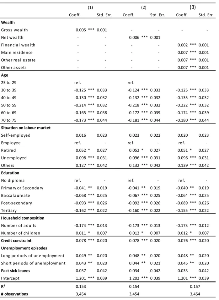
Estimation results are reported in Table 3a (without controlling for income expectations16)
and in Table 3b (controlling for income expectations). Our micro-based estimates show a limited wealth effect on consumption in France: the estimated marginal propensity to consume out of net wealth is about 0.006, meaning that one additional euro of net wealth would be associated with 0.6 cent of euro of additional annual consumption. This result is in line with previous results obtained on aggregate data which range from 0.8 of a cent to 1 cent on annual consumption for every 1 euro increase (Slacalek, 2009; Chauvin and Damette 2010).
[INSERT TABLE 3a]
15 The qualitative indicator of credit constraints is a dummy variable equals to one when the household answers that it was
turned down by a lender or creditor, not given as much credit as applied for, or did not apply for credit because of perceived constraints.
[INSERT TABLE 3b]
Significant marginal propensities to consume out of both financial and housing assets are obtained when considering net wealth components (Table 2a and 2b, column 3). The estimated marginal propensity to consume out of financial wealth seems slightly lower (0.2 cents of a euro) than for other assets (0.7 cents).
The probability to expect an increase in the household total income has a positive significant effect: optimistic households about their future income tend to consume a higher share of their current income, everything else being equal. In our case, the introduction of this variable does not affect the estimated coefficients of the wealth variable. In other words, these results support the views of the existence of direct wealth effect on consumption in addition to the confidence channel.
Socio-demographic variables also have a significant effect on the consumption-to-income ratio. The age effects are significant and indicate a decreasing pattern of the consumption to income ratio over the life course. This age profile could reflect that middle-aged households do save more than younger ones for precautionary motives or for financing consumption in old ages. The negative age effect for older people could reflect a bequest motive. There are also significant differences due to the household composition. In particular the number of adults is negatively correlated with the consumption-to-income ratio, which could be due to some economies of scale. The share of the household income used to finance consumption is higher for unemployed, less educated people, for households facing credit constraints or that encountered unemployment episodes in the past.
These baseline regressions provide average MPC estimated for the whole wealth distribution. However, given the wealth concentration and the changes in asset composition across the wealth distribution illustrated in Section 2, one could suspect that these average
estimates are likely to be affected by some heterogeneity in consumption and saving behaviours across the wealth distribution due for instance to differences in preferences, in precautionary saving or in accumulation for intergenerational transfer motives.
4. Main results: marginal propensity to consume out of wealth across the wealth distribution
We consider now a more flexible specification where we allow the MPC to vary across the net wealth distribution. We define net wealth categories in which the household wealth composition is quite homogeneous (see Fig. 2) and introduce dummy variables accounting for the households belonging to the considered net wealth position which are interacted with the asset values. We consider four net wealth groups defined according to the net wealth percentiles: below median net wealth, p50-p69, p70-p89, and p90-p99. The results are presented in Table 4. We have also considered other ways of splitting the net wealth groups (5 net wealth groups instead of the four ones defined previously) to check for the robustness of the results. It does not affect our main conclusions (see Table C2 in the Appendix C).
[INSERT TABLE 4]
These estimates confirm the significant marginal propensity to consume out of wealth and the differentiated wealth effects depending on the type of assets. Most interestingly, we obtain a decreasing marginal propensity to consume out of wealth along the wealth distribution. Considering the total net value of assets (net wealth), we obtain a MPC decreasing from 3.7 cents of euro (for households below the median net wealth) to about 0.6 cent of euro in the top of the distribution (Table 4, specification A). In other words, the average estimated marginal propensity to consume out of wealth estimated from the baseline
model in Table 3 is likely to be biased by the nonlinear effects arising along the wealth distribution.
Such a pattern is confirmed when disaggregating net wealth into its components (Table 4, Specifications B, C and D). The marginal propensity to consume out of financial wealth decreases from 12.2 cents in the bottom of the wealth distribution to a non-significant effect in the top of the distribution. These differences across the wealth distribution, and especially the large value of MPC in the bottom of the distribution could be due to specific precautionary motives or to credit constraints faced by households with a low level of net wealth17. Financial and housing wealth have differentiated effects which vary across wealth
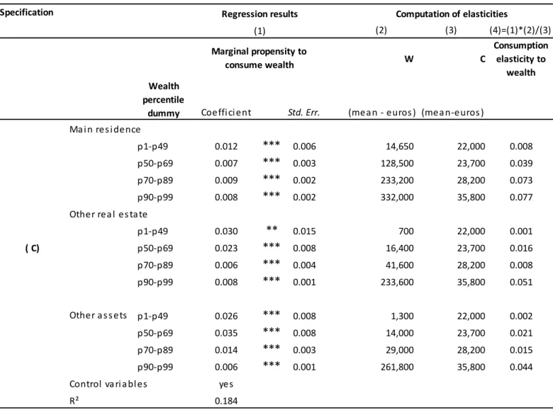
groups (Table 4, Specification B). In the bottom of the wealth distribution, the financial wealth effect dominates the housing one, conversely to the top of the distribution. The heterogeneity is much less pronounced for housing wealth than for financial wealth: the marginal propensity to consume out of housing wealth decreases from 1.4 cent in the bottom of the wealth distribution to 0.8 cent in the top of the distribution. Given that housing assets are not liquid assets, this housing wealth effect could reflect the consumption sensitivity to the “feeling” of being wealthier rather than to effective capital gains. It could also be partly due to a collateral effect. This issue is investigated in Section 5. When disaggregating the housing wealth into “main residence” and “other real estate” (Table 4, Specification C), the MPC decreasing pattern is obtained for both housing components. For a given net wealth group, the MPC out of other real estate is significantly higher than the MPC out of the value of the main residence (except in the p90-p99 wealth group where there is no significant differences between both housing assets). Such a result is coherent with the fact that the wealth component “other real estate” could be more easily liquidated or adjusted by households (as it
is secondary residences and housing assets held for investment purposes) compared with the household main residence.
Once again, the MPC out wealth estimates obtained in the baseline model in Table 3 were not able to capture this heterogeneity along the wealth distribution and across wealth components. In order to investigate the implications for aggregate consumption, we compute the average consumption elasticity to wealth for each wealth group. The average consumption elasticity is obtained by multiplying the estimated MPC by the ratio of the average net wealth out of the average consumption within the considered wealth group (last column of Table 4). The wealth concentration in the top of the distribution (i.e. the fact that the ratio of wealth over consumption, W/C, is sharply increasing along the wealth distribution) counterbalances the decreasing marginal propensity to consume out of wealth. Thus, we obtain an increasing average elasticity of consumption to net wealth (from 0.04 to 0.13 in the top of the net wealth distribution). This increasing pattern seems to be mainly driven by housing assets: the average consumption elasticity to housing wealth increases from 0.01 in the bottom of the net wealth distribution to 0.11 in the top.
When estimating wealth effect on consumption, one potential concern is the spurious correlation that may arise from higher expectations about income and future activity which may be a common determinant of asset prices and consumption. While we already control for household’s income expectations, one could nevertheless worry about a specific correlation arising from housing prices. Following Cooper (2013), we conduct an additional regression which includes geographical variables to account for the fact that some households may feel wealthier than others because they live in more prosperous areas. The available geographical indications on the households’ location in the survey are wide geographical areas (9 regions for France) and the size of the municipalities where the household main residence is located. Adding these explanatory variables does not dramatically change the estimated marginal
propensity to consume out of wealth (see Table C3 in the appendix). The small changes in the estimated coefficient of the household main residence could reflect a correlation between households’ subjective expectations and their subjective evaluation of the value of their main residence.
The potential endogeneity of asset holding decisions is another concern for the robustness of the results. One could suspect that some factors that are not observed or not fully captured by the control variables (such as tastes, time or risk preferences) may affect both consumption and asset allocations. In our case, we are also limited by the survey which does not allow observing the household asset holding decisions over time (as it is a cross-section). This is why we perform additional regressions in order to check whether our results continue to hold when restricting the analysis to households that are holding similar types of assets, i.e. the homeowners and the stockholders (see Table 5). Those estimates confirm the decreasing pattern for MPC, especially as regards the housing wealth for homeowners (from 6.2 cents below median net wealth to 1.2 cent in the p90-p99 group) and financial wealth for stockholders (from 17 cents below median net wealth to 0.4 cent in the top of the distribution).
As expected, for homeowners (respectively for stockholders), we obtain a larger marginal propensity to consume out of the value of housing (resp. financial) wealth than for the full population. For stockholders, we also obtained a MPC out of housing wealth that is closed to the one obtained on the subsample of homeowners, reflecting that most of them (96%) are indeed also homeowners.
[INSERT TABLE 5]
All in all, our empirical analysis sheds light on the MPC heterogeneity across households. The literature points out several factors that could explain such heterogeneity.
First, our results are in line with the framework leading to a concave consumption function with wealth, due to higher precautionary savings for less wealthy households. Second, debt is also deemed to play a role in MPC heterogeneity through two channels. The higher value of the MPC out of financial wealth observed in the bottom of the wealth distribution could reflect liquidity constraints: constrained households cannot adopt their optimal consumption and their consumption is therefore expected to be more sensitive to liquid wealth. The role of housing as collateral for mortgages could lead to heterogeneous MPCs out of housing wealth: higher housing values, everything else being equal, may relax financing constraints faced by households who have contracted loans guaranteed by the value of their housing assets (mortgages). These issues are investigated in the next section.
5. The role of indebtedness 5.1. Debt pressure
In order to investigate whether debt pressure affects consumption behaviors, we split our econometric sample according to two indicators of debt pressure (Table 6):
- The debt-to-asset ratio: we consider a household to be “under pressure” when this ratio is above 2 (which corresponds to the 9th decile of this ratio in the population);
- The debt-service-to-income ratio: we define as “highly indebted” households with a ratio above 25% (which corresponds to the 9th decile of this ratio in the population).
[INSERT TABLE 6]
Concerning financial wealth, the results differ in the bottom and in the top of the wealth distribution. In the bottom of the wealth distribution, highly indebted households (defined according to the debt-to-asset ratio or to the debt-service-to-income ratio) exhibit a non-significant marginal propensity to consume out of financial wealth, while other households have large marginal propensities to consume out of financial wealth. Such a result
may reflect that highly indebted household with low wealth would rather reimburse their debt than consume an additional euro of financial wealth. For higher net wealth deciles (p50-p69 and p70-p89), the MPC out of financial wealth is higher for the samples of highly indebted households, which is in line with the idea that the consumption of liquidity constrained households is more sensitive to liquid wealth.
Concerning housing wealth, larger MPCs are obtained for highly indebted households in the bottom of net wealth distribution, and the other way around in the top wealth group. In the top of the wealth distribution, the results could reflect that wealthy households were able to borrow more without constraining their consumption behavior. Concerning less wealthy people, the results across the subsamples are in line with the assumption that consumption of constrained households is more sensitive to wealth. It would be also in line with a collateral channel affecting the consumption of households relying on debt financing and using housing wealth as collateral.
5.2. Mortgages: a collateral channel in France?
In order to investigate whether the wealth effect on consumption differs across households depending on the type of loans they have contracted, we disentangle households who have loans guaranteed by real estate properties (defined as mortgages) and households without mortgages. We estimate the marginal propensity to consume out of wealth for both sub-populations (Table 7, column 1 and column 2), and obtain larger values of MPC out of housing wealth in the subsample of households that have loans with real estate collateral (Table 7, column 1).
Such a finding may be coherent with a collateral channel that reinforces the direct housing wealth effect: everything else being equal, the consumption of households with mortgages is more sensitive to the value of the housing wealth. Even if our regressions include many variables controlling for observable heterogeneity in net wealth composition, one could nevertheless worry about the fact that the MPC estimated for “non-mortgage households” (Table 7, column 2) results from two types of households that could have very heterogeneous behaviours: homeowners without mortgages (i.e. outright owners or homeowners who rely on other type of loans) and households without any collateralizable real estate property. This is why we conduct an additional regression on the more restricted subsample of households without mortgages but who are nevertheless indebted and who held at least one real estate property (Table 7, column 3). The estimated MPC out of housing wealth for these non-mortgage households are higher than that obtained for the full population of “non-mortgage households” (Table 7, column 2) but it remains lower compared with the estimated MPC of “mortgage households” (Table 7, column 1), in particular in the bottom of the wealth distribution. Such differences in the marginal propensity to consume out of wealth are then consistent with a possible collateral effect which would lead the consumption of “mortgage households” to be more sensitive to housing wealth, everything else being equal.
However, the collateral effect is likely to be limited in France, because the mortgage market is less developed than in some other European countries and is very specific. First, the possibility to use mortgages for financing other assets than the collateralized ones was not permitted by law before 2007 in France, and it has recently been removed in June 2014. It means that using mortgages for financing consumption needs has never been a common practice in France (see also European Central Bank, 2009). Moreover, at the time it was permitted, the value of the collateral could not be reevaluated over time (fixed to the initial collateralized value). Second, when acquiring a property relying on bank loans, two main
types of loans can be contracted: either housing loans which are insured through an insurance scheme18 or mortgages which are collateralized by housing assets. According to the 2010
French Wealth Survey19, most of the loans that were contracted to finance the household main
residence were not mortgages (Table 8): Among the French population, 20.1% of households are indebted to finance the household main residence and only 41.1% of them rely on, at least, one mortgage loan. In other words, 58.9% of households that are indebted to buy their household main residence do not use their real asset as collateral.20 The second main purposes
for which households are indebted in France is for buying cars or other vehicles (20.1% of households). For that purpose, less than 1% of households claim that they use real estate property as collateral. And only about 2% of loans whose main purpose is consumption financing are mortgages.
[INSERT TABLE 8]
Given this institutional background, we suspect that the heterogeneity in the MPC out of housing wealth could reflect a selection effect in the bank lending supply, i.e. mortgages are only offered by banks to very specific households. Indeed, one observes significant differences in the average characteristics of indebted households21 depending on the type of
loans they have, see Table C3 in the Appendix. The “mortgage households” have higher income, housing wealth and total debt. They are also more often self-employed and younger than the other indebted households. The “mortgage households” may also differ in terms of
18 With the insurance scheme, if repayments are missed, the guarantor pays the lender and simultaneously tries to find
amicable solutions to the defaulting problem. In theory, if no solution can be found, the guarantor registers a mortgage by court order at the borrower's expense and the property may be sold to repay the loan. However, in practice, it seems that the entire procedure is very scarcely conducted, so that from the borrower’s point of view there is a clear difference in terms of risk between mortgages and insurance scheme. From the lender perspective, the insurance scheme is also preferred as it covers the household default risk without implying specific measure or provision for the lender in case of default.
19We classify a loan as a mortgage when the household declares that one of the following guaranty is associated with the
loan: “Hypothèque”, “Inscription en privilège de prêteur de deniers”, “bien immobilier”. All other loans are classified as “non mortgages”. 12.6% of households in our econometric sample (i.e. 437 households) have contracted at least one loan which is a mortgage.
20These figures are coherent with a banking survey conducted annually by the Banque de France, in 2010, most of the
distributed loans for acquiring a property were insured through an insurance scheme while only about 30% were guaranteed by a real estate property (mortgages).
21This comparison is done among households holding at least one real estate property (household main residence or other real
unobservable characteristics. They may be more concerned by the value of their housing assets, and may have a more accurate evaluation of their wealth, and in the end, may be more sensitive to it, compared with households that do not provide any real estate collateral.
6. Conclusion
Limited wealth effects on consumption in France are generally found by macro-based estimates using aggregate data on household consumption and wealth. However, households’ wealth is highly concentrated and its composition (in terms of asset categories and debt components) varies a lot across the population. Such heterogeneity cannot be taken into account in macro-based estimates of the marginal propensity to consume out of wealth.
In this paper, we provide micro-based estimates of the marginal propensity to consume out of wealth, controlling for income expectations and investigate its heterogeneity within the population.
As expected, our results confirm the limited wealth effects on consumption in France, driven both by housing and financial wealth. Most interestingly, we obtain a decreasing marginal propensity to consume out of wealth across the wealth distribution. Despite the theoretical work of Carrol and Kimball (1996), empirical evidences of such a pattern are scarce in the literature.
Moreover, we contribute to the debate on which wealth effect is the largest one (housing or financial wealth effects) and show that the answer depends on the position of households in the wealth distribution. In the bottom of the net wealth distribution, the marginal propensity to consume out of financial wealth dominates the housing wealth effect; while in the top of the net wealth distribution, the marginal propensity to consume out of financial wealth is not significant. The pattern of wealth effects looks slightly different in terms of consumption elasticity to wealth, as the wealth concentration in the top of the distribution counterbalances the decreasing marginal propensity to consume out of wealth.
Taken together, the heterogeneity in the MPC and in the consumption elasticity has various policy implications. On the one hand, the decreasing MPC indicates that the consumption of some sub-populations (the less wealthy ones) is more sensitive to a change in their asset values. This is why public policies (monetary policy on interest rate or fiscal policy on asset revenues for instance) could have distributive effects within the population. Heterogeneous MPC are then key factors to be taken into account to analyse the transmission of wealth shocks to aggregate consumption (See European Central Bank, 2014). On the other hand, our computed elasticity which reflects the wealth concentration within the population indicates that the consumption reaction of rich people plays a key role for the overall wealth effect on consumption at the aggregate level. We argue that such heterogeneities have to be taken into account when performing welfare analysis.
Fig 1. Observed (HBS) and imputed distribution (FWS) of non durable consumption
Fig 2. Average gross wealth composition by gross wealth percentiles in France
Source: French Wealth Survey (Enquête Patrimoine 2010) - Whole population - Weighted statistics. Housing assets: household main residence and other real estate property than the household main residence (holiday homes, rental homes, excluding real estate property held for business purposes). Financial assets: deposits, mutual funds, shares, voluntary private pensions, whole life insurance and other financial assets (excluding business assets). Other assets: assets held for business purposes (land, farms, office space rented out to businesses, etc.) and valuables.
Table 1. Distributions of non-durable consumption, net wealth and income
Source: French Wealth Survey (Enquête Patrimoine 2010) and Household Buget Survey (Enquête Budget de famille 2006)- Whole population - Weighted statistics.
Table 2. Mean values of gross and net wealth and share of asset categories and debt in total across the wealth distribution
Source: French Wealth Survey (Enquête Patrimoine 2010) - Whole population - Weighted statistics
Financial assets: deposits, mutual funds, shares, voluntary private pensions, whole life insurance and other financial assets (excluding business assets). Other housing assets: other real estate property than the household main residence (holiday homes, rental homes, excluding real estate property held for business purposes). Other assets: assets held for business purposes (land, farms, office space rented out to businesses, etc.) and valuables. Debt: all various forms of debt contracted by the household (mortgage debt, non-collateralized debt including debt contracted for business purposes).
Non durable
consumption Net wealth
Total Income Excl. Capital income
Mean (euros) 24,500 229,300 36,900 32,700 Median (euros) 22,300 114,500 29,200 26,900 P90/Median 1.99 4.42 2.20 2.16 Gini 0.33 0.65 0.38 0.36 Income Gross wealth percentiles
Gross wealth Net wealth Financial wealth Main residence Other housing assets Other Assets Debt 0-25 9,700 -700 0.61 0.00 0.00 0.39 0.15 25-50 76,100 49,400 0.34 0.36 0.05 0.25 0.13 50-70 208,500 174,400 0.16 0.66 0.05 0.13 0.16 70-90 370,800 340,200 0.15 0.60 0.09 0.16 0.12 90-99 876,200 812,600 0.17 0.44 0.22 0.17 0.10 99-100 4,486,200 4,256,200 0.26 0.22 0.26 0.27 0.07 All 259,000 229,300 0.20 0.48 0.14 0.18 0.12
Table 3a. Marginal propensity to consume out of wealth: baseline results
Dependent variable: ratio of non-durable consumption to income (excluding income from financial and housing assets). OLS estimates. Significant at ***1%, **5% and *10%. Econometric sample.
(1) (2) (3)
Coeff. Std. Err. Coeff. Std. Err. Coeff. Std. Err.
Wealth Gros s wea l th 0.005 *** 0.001 - - - -Net wea l th - - 0.006 *** 0.001 Fi na nci a l wea l th - - - - 0.002 *** 0.001 Ma i n res i dence - - - - 0.007 *** 0.001 Other rea l es ta te - - - - 0.007 *** 0.001 Other a s s ets - - - - 0.007 *** 0.001 Age 25 to 29 ref. ref. 30 to 39 -0.125 *** 0.033 -0.124 *** 0.033 -0.125 *** 0.033 40 to 49 -0.130 *** 0.032 -0.132 *** 0.032 -0.135 *** 0.032 50 to 59 -0.214 *** 0.032 -0.218 *** 0.032 -0.222 *** 0.032 60 to 69 -0.165 *** 0.038 -0.172 *** 0.039 -0.174 *** 0.039 70 to 75 -0.173 *** 0.044 -0.181 *** 0.044 -0.180 *** 0.044
Situation on labour market
Sel f-empl oyed 0.016 0.023 0.023 0.022 0.020 0.023 Empl oyee ref. - ref. - ref. - Reti red 0.052 * 0.027 0.052 * 0.027 0.051 * 0.027 Unempl oyed 0.098 *** 0.031 0.096 *** 0.031 0.096 *** 0.031 Others 0.127 *** 0.042 0.132 *** 0.042 0.139 *** 0.042
Education
No di pl oma ref. - ref. - ref. - Pri ma ry or Seconda ry -0.041 ** 0.019 -0.041 ** 0.019 -0.040 ** 0.019 Ba cca l a urea te -0.068 *** 0.025 -0.067 *** 0.025 -0.064 *** 0.025 Pos t-s econda ry -0.093 *** 0.026 -0.092 *** 0.026 -0.089 *** 0.026 Terti a ry -0.162 *** 0.022 -0.160 *** 0.022 -0.155 *** 0.022 Household composition Number of a dul ts -0.174 *** 0.013 -0.173 *** 0.013 -0.173 *** 0.012 Number of chi l dren 0.011 * 0.007 0.012 * 0.007 0.012 * 0.007
Credit constraint 0.078 *** 0.020 0.078 *** 0.020 0.076 *** 0.020
Unemployment episodes
Long peri ods of unempl oyment 0.049 ** 0.020 0.048 ** 0.020 0.048 ** 0.020 Short peri ods of unempl oyment 0.043 ** 0.020 0.044 ** 0.021 0.045 ** 0.020
Past sick leaves 0.037 0.042 0.034 0.042 0.033 0.042
Intercept 1.201 *** 0.039 1.202 *** 0.039 1.201 *** 0.039
R² 0.153 0.154
# observations 3,454 3,454
0.157 3,454
Table 3b. Marginal propensity to consume out of wealth: baseline results accounting for subjective income expectations
Dependent variable: ratio of non-durable consumption to income (excluding income from financial and housing assets). OLS estimates. Significant at ***1%, **5% and *10%. Econometric sample. .
(1) (2) (3)
Coeff. Std. Err. Coeff. Std. Err. Coeff. Std. Err.
Wealth Gros s wea l th 0.005 *** 0.001 - - - -Net wea l th - - 0.006 *** 0.001 Fi na nci a l wea l th - - - - 0.002 *** 0.001 Ma i n res i dence - - - - 0.007 *** 0.001 Other rea l es ta te - - - - 0.007 *** 0.001 Other a s s ets - - - - 0.007 *** 0.001
Positive income expectations 0.002 ** 0.001 0.002 ** 0.001 0.002 ** 0.001 Age 25 to 29 ref. ref. 30 to 39 -0.096 *** 0.036 -0.093 *** 0.034 -0.095 *** 0.036 40 to 49 -0.070 * 0.045 -0.068 * 0.045 -0.072 * 0.045 50 to 59 -0.127 ** 0.055 -0.127 ** 0.054 -0.131 ** 0.055 60 to 69 -0.063 0.065 -0.064 0.065 -0.065 0.065 70 to 75 -0.061 0.072 -0.062 0.072 -0.060 0.072
Situation on labour market
Sel f-empl oyed 0.030 0.024 0.038 * 0.024 0.035 0.024
Empl oyee ref. ref. - ref. -
Reti red 0.063 ** 0.028 0.063 ** 0.028 0.063 ** 0.028
Unempl oyed 0.103 *** 0.031 0.101 *** 0.031 0.101 *** 0.031
Others 0.145 *** 0.043 0.150 *** 0.043 0.157 *** 0.043
Education
No di pl oma ref. - ref. - ref. -
Pri ma ry or Seconda ry -0.042 ** 0.019 -0.041 ** 0.019 -0.040 ** 0.019 Ba cca l a urea te -0.068 *** 0.025 -0.067 *** 0.025 -0.064 *** 0.025 Pos t-s econda ry -0.088 *** 0.026 -0.086 *** 0.026 -0.083 *** 0.026 Terti a ry -0.164 *** 0.022 -0.162 *** 0.022 -0.157 *** 0.022 Household composition Number of a dul ts -0.174 *** 0.013 -0.173 *** 0.013 -0.173 *** 0.012
Number of chi l dren 0.009 0.007 0.009 0.007 0.009 0.007
Credit constraint 0.079 *** 0.020 0.079 *** 0.020 0.078 *** 0.020
Unemployment episodes
Long peri ods of unempl oyment 0.049 *** 0.020 0.049 ** 0.020 0.049 ** 0.020 Short peri ods of unempl oyment 0.044 * 0.020 0.044 ** 0.021 0.045 ** 0.020
Past sick leaves 0.032 ** 0.042 0.029 0.042 0.028 0.042
Intercept 1.002 *** 0.102 1.007 *** 0.102 1.004 *** 0.102
R² 0.154 0.155
# observations 3,454 3,454
0.158 3,454
Table 4. Marginal propensity to consume out of wealth and average elasticity across the wealth distribution (2) (3) (4)=(1)*(2)/(3) W C Consumption elasticity to wealth Wealth percentile
dummy Coeffi ci ent Std. Err. (mea n - euros ) (mea n-euros ) Net wea l th p1-p49 0.037 *** 0.005 25,900 22,014 0.044 p50-p69 0.013 *** 0.002 181,000 23,700 0.096 (A) p70-p89 0.010 *** 0.001 354,150 28,200 0.123 p90-p99 0.006 *** 0.001 846,200 35,800 0.133 Control va ri a bl es yes R² 0.168 Fi na nci a l a s s ets p1-p49 0.122 *** 0.014 8,000 22,000 0.044 p50-p69 0.020 *** 0.008 26,400 23,700 0.022 p70-p89 0.013 ** 0.006 52,800 28,200 0.024 p90-p99 0.002 0.001 178,100 35,800 0.009 Hous i ng wea l th p1-p49 0.014 ** 0.006 14,650 22,000 0.009 (B) p50-p69 0.009 *** 0.002 139,700 23,700 0.051 p70-p89 0.008 *** 0.002 269,800 28,200 0.080 p90-p99 0.008 *** 0.001 519,300 35,800 0.116 Other a s s ets p1-p49 0.025 ** 0.008 1,300 22,000 0.002 p50-p69 0.035 *** 0.008 14,000 23,700 0.020 p70-p89 0.014 *** 0.003 29,000 28,200 0.015 p90-p99 0.006 *** 0.001 261,800 35,800 0.044 Control va ri a bl es yes R² 0.175
Specification Regression results
(1)
Marginal propensity to consume wealth
Table 4 (continued). Marginal propensity to consume out of wealth and average elasticity across the wealth distribution
Dependent variable: ratio of non-durable consumption to income (excluding income from financial and housing assets). Other control variables: income expectations, age, work status, education of the reference person, household composition, credit constraint, unemployment episodes, sick leaves.
OLS estimates. Econometric sample. Significant at ***1%, **5% and *10%. . (2) (3) (4)=(1)*(2)/(3) W C Consumption elasticity to wealth Wealth percentile
dummy Coeffi ci ent Std. Err. (mea n - euros ) (mea n-euros ) Ma i n res i dence
p1-p49 0.012 *** 0.006 14,650 22,000 0.008 p50-p69 0.007 *** 0.003 128,500 23,700 0.039 p70-p89 0.009 *** 0.002 233,200 28,200 0.073 p90-p99 0.008 *** 0.002 332,000 35,800 0.077 Other rea l es tate
p1-p49 0.030 ** 0.015 700 22,000 0.001 ( C) p50-p69 0.023 *** 0.008 16,400 23,700 0.016 p70-p89 0.006 *** 0.004 41,600 28,200 0.008 p90-p99 0.008 *** 0.001 233,600 35,800 0.051 Other a s s ets p1-p49 0.026 *** 0.008 1,300 22,000 0.002 p50-p69 0.035 *** 0.008 14,000 23,700 0.021 p70-p89 0.014 *** 0.003 29,000 28,200 0.015 p90-p99 0.006 *** 0.001 261,800 35,800 0.044 Control va ri a bl es yes R² 0.184 Computation of elasticities Marginal propensity to consume wealth
Specification Regression results
Table 5. Marginal propensity to consume out of wealth : subsamples of homeowners and stockholders
Dependent variable: ratio of non-durable consumption to income (excluding income from financial and housing assets). Other control variables: income expectations, age, work status, education of the reference person, household composition, credit constraint, unemployment episodes, sick leaves.OLS estimates Significant at ***1%, **5% and *10%.
Wealth variables Wealth
percentile Homeowners Stockholders
(1) (2) Coeff. Coeff. Std. Err. Std. Err. Fi na nci a l Wea l th p1-p49 0.086 *** 0.170 *** 0.030 0.032 p50-p69 0.023 * 0.018 0.012 0.015 p70-p89 0.023 *** 0.023 *** 0.006 0.009 p90-p99 0.004 *** 0.004 *** 0.001 0.002 Hous i ng wea l th p1-p49 0.062 *** 0.055 * 0.007 0.034 p50-p69 0.031 *** 0.032 *** 0.003 0.009 p70-p89 0.019 *** 0.020 *** 0.002 0.004 p90-p99 0.012 *** 0.012 *** 0.001 0.001 Other wea l th p1-p49 0.013 * 0.023 0.008 0.055 p50-p69 0.030 *** 0.032 0.010 0.039 p70-p89 0.013 *** 0.031 *** 0.003 0.009 p90-p99 0.007 *** 0.008 *** 0.001 0.002 Control va ri a bl es yes yes R² 0.266 0.302
Table 6. Differences across households groups: debt pressure
Dependent variable: ratio of non-durable consumption to income (excluding income from financial and housing assets). Other control variables: income expectations, age, work status, education of the reference person, household composition, credit constraint, unemployment episodes, sick leaves.
OLS estimates. Significant at ***1%, **5% and *10%. Econometric sample
Wealth variables Wealth percentile ratio>2 ratio<2 ratio >0,25 ratio <0,25
Coeff. Coeff. Coeff. Coeff.
Std. Err. Std. Err. Std. Err. Std. Err. Fi na nci a l Wea l th p1-p49 0.017 0.117 *** 0.041 0.124 ** 0.044 0.015 0.062 0.015 p50-p69 0.068 ** 0.021 *** 0.030 0.021 *** 0.034 0.008 0.041 0.008 p70-p89 0.042 *** 0.013 ** 0.054 ** 0.013 *** 0.016 0.006 0.022 0.006 p90-p99 0.002 0.001 0.004 0.000 0.003 0.001 0.002 0.001 Hous i ng wea l th p1-p49 0.032 ** 0.016 ** 0.041 *** 0.013 *** 0.016 0.007 0.016 0.007 p50-p69 0.03 *** 0.009 *** 0.019 ** 0.010 *** 0.007 0.003 0.007 0.003 p70-p89 0.018 *** 0.008 *** 0.010 ** 0.009 *** 0.005 0.002 0.004 0.002 p90-p99 0.013 *** 0.007 *** 0.007 *** 0.009 *** 0.002 0.001 0.002 0.001 Other wea l th 0.006 *** 0.007 0.006 *** 0.008 *** 0.002 0.002 0.002 0.001
Control va ri a bl es yes yes yes yes
R² 0.258 0.177 0.227 0.184
#obs erva tions 550 2904 527 2927
Table 7. Differences across households groups: indebtedness and collateral
Dependent variable: ratio of non-durable consumption to income (excluding income from financial and housing assets). Other control variables: income expectations, age, work status, education of the reference person, household composition, credit constraint, unemployment episodes, sick leaves. In column 1, the econometric sample is restricted to the households with at least one mortgage (i.e. a loan with one of the following associated guaranties: “Hypothèque”, “Inscription en privilège de prêteur de deniers”, “bien immobilier” while the results for the other households (without mortgages are in column 2). Column 3 reports the results for a sub-population of column 2: households without mortgages but who are nevertheless indebted and have at least one real estate property. OLSE estimates. Significant at ***1%, **5% and *10%. Econometric sample
Wealth variables Wealth percentile With loans guarantied by real estate collateral All (1) (2) (3)
Coeff. Coeff. Coeff.
Std. Err. Std. Err. Std. Err.
Fi na nci a l Wea l th p1-p49 0.045 0.117 *** 0.204*** 0.079 0.015 0.047 p50-p69 0.060* 0.021 *** 0.018 0.036 0.008 0.026 p70-p89 0.042** 0.013 ** 0.028** 0.019 0.006 0.011 p90-p99 0.005 0.001 0.004** 0.004 0.001 0.002 Hous i ng wea l th p1-p49 0.078*** 0.012 * 0.048*** 0.019 0.006 0.011 p50-p69 0.034*** 0.010 *** 0.032*** 0.010 0.003 0.005 p70-p89 0.020*** 0.008 *** 0.021*** 0.005 0.002 0.003 p90-p99 0.012*** 0.008 *** 0.011*** 0.002 0.001 0.001 Other wea l th 0.008*** 0.007 *** 0.009*** 0.002 0.001 0.001
Control va ri a bl es yes yes yes
R² 0.227 0.178 0.247
#obs erva tions 437 3,017 1,166
Indebted households with a real estate property Without loans guarantied by real
Table 8. Percentage of indebted households
Purpose of the loans
% of households with one loan (or more)
contracted for the following purpose
% of households with at least one mortgage for financing the associated purpose (among HH declaring the associated purpose)
Main residence 20.1 41.2
Other real estate 6.3 36.9
Renovation works 6.8 7.4
Cars, vehicles 20.1 0.5
Others (consumption) 9.9 2.3
Business 5.6 2.6
All purposes 47.6 22.7
Among the French population, 20.1% of households are indebted to finance the household main residence. Among these households, 41.1% rely on, at least, one mortgage loan (defined as loan with one of the following associated guaranty “hypothèque”, “Inscription en privilege de prêteurs de deniers” or “bien immobilier”). Source: French Wealth Survey (Insee) - Whole population -Weighted statistics.