The value of the greenbelt in Vienna: a spatial hedonic analysis

HAL Id: halshs-00939270

https://halshs.archives-ouvertes.fr/halshs-00939270v2

HAL is a multi-disciplinary open access archive for the deposit and dissemination of sci-entific research documents, whether they are pub-lished or not. The documents may come from teaching and research institutions in France or abroad, or from public or private research centers.

L’archive ouverte pluridisciplinaire HAL, est destinée au dépôt et à la diffusion de documents scientifiques de niveau recherche, publiés ou non, émanant des établissements d’enseignement et de recherche français ou étrangers, des laboratoires publics ou privés.

analysis

Shanaka Herath, Johanna Choumert, Gunther Maier

To cite this version:

Shanaka Herath, Johanna Choumert, Gunther Maier. The value of the greenbelt in Vienna: a spatial hedonic analysis. 2015. �halshs-00939270v2�

C E N T R E D'E T U D E S E T D E R E C H E R C H E S S U R L E D E V E L O P P E M E N T I N T E R N A T I O N A L

SERIE ETUDES ET DOCUMENTS DU CERDI

THE

VALUE

OF

THE

GREENBELT

IN

VIENNA:

A

SPATIAL

HEDONIC

ANALYSIS

Shanaka HERATH, Johanna CHOUMERT, Gunther MAIER

Etudes et Documents n° 02

January 2014

CERDI

65 BD. F. MITTERRAND

63000 CLERMONT FERRAND - FRANCE TÉL. 0473177400

FAX 0473177428

2

The authors

Shanaka Herath, Faculty of the Built Environment, City Futures Research Centre, University

of New South Wales, Sydney 2052, Australia

Email:

shanaka.herath@unsw.edu.au

Johanna Choumert, Clermont Université, Université d'Auvergne, CNRS, UMR 6587, CERDI,

F-63009 Clermont Fd

Email:

johanna.choumert@udamail.fr

Gunther Maier, Research Institute for Spatial and Real Estate Economics / Institute for the

Environment and Regional Development, WU-Vienna University of Economics and Business,

Augasse 2-6, 1090 Vienna, Austria

Email:

gunther.maier@wu.ac.at

La série des Etudes et Documents du CERDI est consultable sur le site :

http://www.cerdi.org/ed

Directeur de la publication : Vianney Dequiedt

Directeur de la rédaction : Catherine Araujo Bonjean

Responsable d’édition : Annie Cohade

ISSN : 2114 - 7957

Avertissement :

Les commentaires et analyses développés n’engagent que leurs auteurs qui restent seuls

responsables des erreurs et insuffisances.

This work was supported by the LABEX IDGM+ (ANR-10-LABX-14-01) within the program “Investissements d’Avenir” operated by the French National Research Agency (ANR)

3

Abstract

This paper employs the hedonic price method (HPM) to examine whether the implicit value of the greenbelt is capitalized into apartment prices in the city of Vienna, Austria. We improve the traditional model using spatial econometric techniques and compare estimates from different spatial models, namely the spatial lag model (SAR), the spatial error model (SEM) and the spatial Durbin model (SDM). While our use of spatial models addresses the common problem of omitted variable bias, the SDM specifically allows for controlling possible nearby proximity effects (i.e., small-scale neighbourhood) that are rarely included in this type of analyses. Findings indicate that distance from the greenbelt is important in explaining apartment prices in Vienna: while the CBD exerts a centripetal force, the greenbelt, on the contrary, exerts a centrifugal force. The SDM is found to be the best performing model indicating existence of small-scale neighbourhood effects and presenting a solid case for consideration of this model in valuation of green amenities.

Keywords

Greenbelt, open space, urban amenities, hedonic price valuation, spatial econometrics, spatial Durbin model

JEL

4

1. Introduction

Green spaces are a response for or a resistance against continuous expansion of urban areas accompanied by profound economic and social movements. In Austria, a country that remained predominantly rural until the Second World War, the share of the urban population has now reached 68% of the total population (World Bank Data1). This demographic shift from rural to urban areas is accompanied by a decline in natural and agricultural lands, and transformation of landscapes. Located away from a direct and immediate access to natural amenities, the urban population is likely to feel the need to have ‘a place of nature’ close to where they live. Green spaces are therefore an important part of the overall sustainable development plan: they contribute to economic attractiveness (Crompton et al. 1997; Crompton 2000), promote social ties (Maas et al. 2009)2 and provide landscape as well as environmental3 amenities (Bolund and Hunhammar 1999; Jim and Chen 2008; Jo and McPherson 1995; Tzoulas et al. 2007; Zhang et al. 2007) and health benefits (De Vries et al. 2003; Kuo and Sullivan 2001; Willis and Osman 2005; Maas et al. 2006; Tzoulas et al. 2007).4

Greenbelts are a special type within the taxonomy of open spaces. According to McConnell and Wells (2005, p. 17), a greenbelt can be defined as “an area of open space surrounding an urban area and preserved from development. It is used to define the edge of the urban fringe, at least until that time when development ‘leapfrogs’ over the greenbelt. Greenbelts are also referred to as ’urban growth boundaries‘. It contains the physical expansion of the urbanized area and is thus considered an essential outcome of the containment policy (Nelson 1988).5 This role of the greenbelt as an instrument in the containment policy is well established in the literature. For instance, Kuhn (2003) states that greenbelts are designed to protect a compact urban form while Pendall and Martin (2002)

1

http://data.worldbank.org/

2

Maas et al. (2009) present the results of a study conducted in the Netherlands on 10,089 individuals. They find a correlation between lack of green spaces (within 3 km of the place of residence) and the feeling of loneliness and lack of social ties. Other studies also show that there is less domestic violence reported in green neighbourhoods (Prow 1999; Kuo and Sullivan 2001). Witt and Crompton (1996) highlight a correlation between the presence of green spaces and crime: juvenile delinquency and domestic violence are mitigated in green neighbourhoods.

3

Ecological services in urban areas are air filtration, regulation of microclimate, noise reduction, water retention, water treatment, carbon sequestration, erosion control and preservation of biodiversity.

4

Willis and Osman (2005) present a review of the literature on the positive effects of green spaces on health. Proximity to green spaces promotes physical activities. Potential benefits include reduced risk of cardiovascular disease, certain cancers, certain types of diabetes, etc. A pleasant living environment has positive effects on mental health and well-being. The presence of a green space can reduce the risk of depression. They estimate that a 1% permanent reduction in the sedentary population of the United Kingdom from 23% to 22% would produce a social benefit of 1.44 billion pounds per year and 479 million if the elderly are excluded. This does not include benefits related to the reduction of psychological morbidity such as mental illness, domestic violence or mental fatigue. These figures show that the benefits of green spaces are substantial.

5

Urban containment policies have been classified by Pendall and Martin (2002) into three major forms: urban growth boundaries, urban service boundaries and greenbelts.

5 assert that greenbelts are physical boundaries entailing open spaces around cities. From a planning point of view, a greenbelt usually refers to a passage drawn fairly tightly around a city or urban region that planners intend to be permanent or at least very difficult to change (Pendall and Martin 2002). “A greenbelt is a zone of land around the city where building development is severely restricted (Amati and Yokohari 2006, p. 125)” and, it thus refers to a physical area of open space, e.g., farmland, forest or other green space, that surrounds a city or metropolitan area, and it is intended to be a permanent barrier to urban expansion (Bengston and Youn 2006).

Additionally, a greenbelt can also be the outcome of an urban policy that is intended for preserving green spaces for environmental and recreation purposes. In the context of reducing environmental pollution, a greenbelt has been described as “a strip of trees of such species, and such a geometry, that when planted around a source, would significantly attenuate the air pollution by intercepting and assimilating the pollutants in a sustainable manner” (Abbasi and Khan 2000, p. 1). In Vienna, these environmental and recreational purposes seem to have been dominant compared to the containment aspect of the greenbelt. This is indicated in the official policy documents – “In 1995, the Vienna City Council approved the Green Belt Masterplan… (that) foresees the conservation of whole land tracts or contiguous portions of land as recreational areas and ecologically valuable zones, which are to be kept free of buildings” (City of Vienna 2000, pp. 33).

Production costs of such public amenities are well known (costs of planting trees, hedge cuts etc.) and easily measurable. Benefits are more difficult to assess. These benefit assessments though are of crucial value to policy makers: they provide information on public preferences and, allow for prioritizing and calibrating local policies. The objective of this paper is to analyse home-buyers’ willingness to pay for the greenbelt in Vienna. In the literature, two types of methods have been developed for the assessment of preferences and for valuing greenbelts. The contingent valuation method (Hanley and Knight 1992) and the choice experiments method (Bullock 2008) are based on stated preferences while the hedonic price method (HPM) (Correl et al. 1978; Willis and Whitby 1985) and the travel costs method (Dwyer et al. 1983) are based on revealed preferences. Given our concern is related to the use of land resources and urban pressure, we seek to determine the residential value of the greenbelt using the HPM.

Our contribution is twofold. Firstly, we examine how the households negotiate the trade-off between proximity to the central business district (CBD) and the greenbelt. As shown in existing studies, close proximity to a greenbelt tends to generally increase house prices. However, empirical evidence is scarce with respect to assessing benefits of both proximity to the greenbelt and the CBD within the same modelling framework. Also, the majority of hedonic studies have focused on

6 evaluating the effect of proximity to various green spaces other than greenbelts. As a policy discourse around greenbelts is re-emerging in other European cities6, this study is of relevance to those contexts as well. Secondly, our analysis deals with apartment prices in a spatial context. It is shown in spatial econometrics that values observed at points or regions tend to depend on values of nearby observations. Thus, models that ignore this spatial dependence among nearby observations are likely to produce inefficient and unbiased parameter estimates (Anselin 1988). To address this issue we use spatial hedonic models in our valuation of the greenbelt. While the spatial models redress the common problem of omitted variable bias, one of the models we use – i.e., the spatial Durbin model – specifically allows for controlling possible nearby proximity effects (i.e., small-scale neighbourhood) that are rarely included in this type of analyses.

There have been several recent hedonic pricing studies for Vienna although none of them either specifically assessed the value of the greenbelt or controlled for nearby proximity effects of the small-scale neighbourhood. Brunauer et al. (2009) used a hedonic framework to assess nonlinear price functions and spatial heterogeneity in the rental market. Results showed that there was a substantial spatial variation within the rental market in Vienna. District-specific heterogeneity was accounted for using location specific intercepts with the postal code serving as a location variable. Herath and Maier (2013) found that district-specific characteristics and distance from the CBD were important in explaining apartment prices in Vienna. Spatial hedonic methods were used in that study although the primary aim was to estimate the rent-gradient with and without spatial effects. Additionally, Wieser’s (2006) study found that prices in the residential land market in Vienna were substantially affected by the proximity to the underground network, accessibility to open spaces and shopping centres, and even announcements of new subway stations. Wieser included distance from the nearest open space (a park, the greenbelt or other major recreational area) although failed to consider the exclusive impact of proximity to the greenbelt within the study. A study by Feilmayr (2004) utilized the HPM only in the context of constructing house price indices for Vienna.

The remainder of the paper is structured as follows: The next section presents a brief literature survey; Section 3 and Section 4 describe data and variables used and the empirical models employed. The results are discussed in Section 5, and the paper concludes in Section 6.

6

The city of Paris, France, has also laid plans to develop a greenbelt. This Greater Paris project was presented by the Government in 2009. It aims at portraying Paris as a model of a sustainable city with efficient transportation, a competitive economy, better quality of life, a stronger cultural life and increased presence of nature in the city. While transportation is the key element of the project, the role of green spaces has also been recognized as important: beyond the preservation of the existing green spaces, it is intended to promote the development of a greenbelt inclusive of regional parks and forests to create ecological corridors for fauna and flora.

7

2. Literature survey

Numerous studies investigate the implicit value of greenbelts, forests, open spaces, parks and wetlands (For surveys see Fausold and Lilieholm 1999; McConnell and Walls 2005; Rambonilaza 2004; Choumert and Salanié 2008; Brander and Koetse 2011; and Waltert and Schläpfer 2010). Since urban forests, grasslands and wetlands usually demarcate part of the greenbelt, we consider these land uses as similar to the greenbelt within the scope of this study. Other amenities such as open spaces and parks also serve similar environmental and recreational services to a greenbelt or a forest but on a smaller scale (Morancho 2003).

In an overview paper, Nelson (1985) documents that a greenbelt increases the value of urban land in proximity and this effect also extends to the exurban land market. He maintains, however, that value of land located within the greenbelt is likely lower due to large-lot zoning and restrictions on agricultural practices. An early study by Correll et al (1978) asserts that the existence of a greenbelt has a significant positive impact on nearby residential property values in Boulder, Colorado. The residential property units adjacent to the greenbelt are valued 32% more on average than the property units approximately 1 km away. Assuming a linear relationship, the authors argue that property prices decreased by $13.75 for each meter away from the greenbelt. With reference to the interaction between the greenbelt and land values in Washington County, Oregon area, Nelson (1988) empirically argues that exurban land values benefit from the proximity to the greenbelt while the greenbelt land value is not adversely affected by the proximity to the exurban development.

These hedonic valuations concerning greenbelts go beyond the US context. For example, Tyrvainen (1997) and Tyrvainen and Miettinen (2000) document that urban forests are appreciated as an environmental characteristic within two Finnish regions. These studies use the HPM to implicitly estimate the value of urban forest amenities by comparing dwelling prices and specific amounts of amenities associated with dwelling units. The former study reports that proximity of watercourses and wooded recreation areas as well as increasing proportion of total forested area in a housing district have a positive influence on apartment price while the latter states that one kilometre increase in the distance to the nearest forested area leads to an average 5.9% decrease in the market price of the dwelling. It is also found that dwellings with a view onto forests are 4.9% more expensive on average than dwellings with otherwise similar attributes (Tyrvainen and Miettinen 2000). In another study, Garrod and Willis (1992) demonstrate the value of British urban forests as a source of aesthetic enjoyment. They examine the amenity value of forestry and woodland environments through their effect on house prices. A two-stage hedonic price model is

8 applied and the impact of forest type on house prices is explored. This research indicates that the impact of woodland on housing values is significant. The effects are investigated for three types of trees: Sitka spruce depresses house prices by approximately £141 for every unit increase in relative cover; broadleaved trees add approximately £43 per unit increase in relative cover; and the relative proportion of larch (and pine) does not significantly affect house prices.

Valuable welfare, urban planning and/or policy insights are often drawn through hedonic studies. Some of these analyses estimate premiums associated with certain environmental amenities and then present related policy discourse. Based on a hedonic framework and using a time series of property values, Lee and Linneman (1998) document evidence that the value of the greenbelt in Seoul, South Korea changes over time. The marginal price of accessibility to the greenbelt which showed an increasing trend until 1980s started to decrease over time since then. In addition to providing empirical support for the positive amenity value of urban greenbelt, this study provides policy and welfare related insights such as those greenbelt amenities are congestible and the cost of the congestion of the area inside the greenbelt changes over time. Through a unique study of rents of rural self-catering cottages (“gites”), Le Goffe (2000) estimates the external effects of agricultural and silvicultural activities in the French region Britanny. The results indicate that the price of cottages is negatively influenced by intensive fodder and livestock farming but positively related to permanent grassland. Possible welfare outcomes are discussed by way of comparison of the levels of implicit prices against the likely rate of the economic incentives. One of the cases conferred is a comparison of the marginal benefit of the increase of permanent grassland to the subsidy allotted for converting arable land into permanent grassland, results showing that the benefit is superior to the subsidy considered.

The majority of available hedonic studies are non-spatial in nature despite the growing popularity of spatial analysis and emerging use of spatial techniques for analysing housing markets. Anselin (1988) among others has shown that disregarding the spatial relationship when there exists a spatial dependence can lead to inefficient parameter estimates. There is a growing use of spatial econometrics in the recent hedonic literature, particularly several studies on the value of green amenities. Among them, Kadish and Netusil (2012) and Pandit et al. (2013) report that urban trees have a positive impact on real estate prices while Melichar and Kaprová (2013) and Sander and Haight (2012) establish positive effects of urban greenery on home values.

9

3. Data and variables

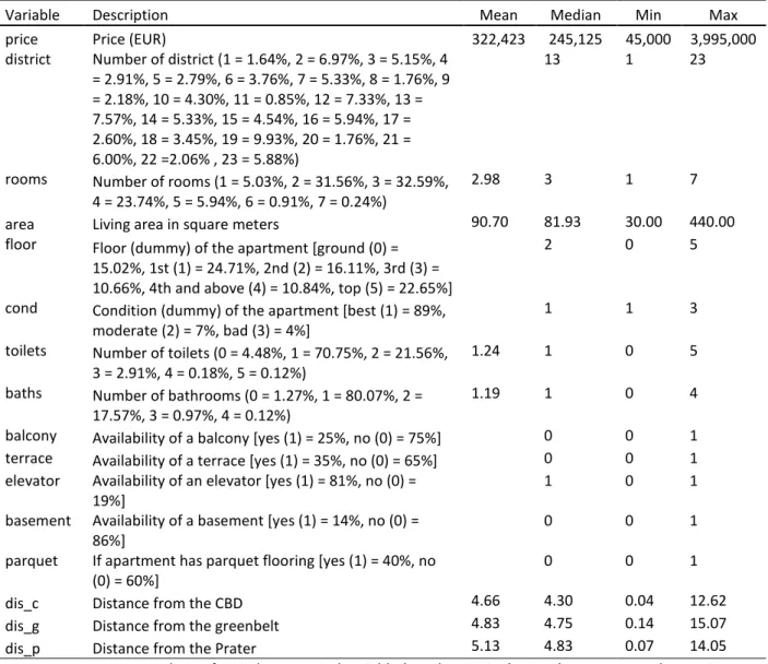
The dataset is provided by the real estate agency ERES NETconsulting-Immobilien.NET GmbH in Vienna. It includes 1651 apartments that were available for sale within the Vienna city limits over the period from December 11, 2009 to March 25, 2010. The dataset comprises the asking price of each apartment and intrinsic characteristics: number of rooms; living area in square meters; the floor (level); condition of the apartment (bad, moderate or good); number of toilets; number of bathrooms; availability of a balcony, terrace, elevator, basement; and availability of parquet flooring. The physical address of each apartment is also included. This information is required to generate longitude and latitude coordinates associated with apartment units, to calculate distance between different points in space, and to create different types of measures of apartment location.

Assessed values including owner assessments of house prices are often used in the absence of transaction prices in housing studies (see Orford 1999; Henneberry 1998; Cheshire and Sheppard 1989). As our study focuses on spatial variation of apartment prices, use of asking prices does not pose any problem unless there is a systematic variation across space in the difference between the owners assessed value and the actual price. Asking prices are close proxies for transaction prices also due to theoretical reasons. Since suppliers desire to sell their houses with the shortest time, they unwittingly project the behaviour of potential buyers when setting the asking price. Setting it too high will result in attracting fewer offers, ultimately costing more to keep the house on the market for a longer time. The supplier loses when the asking price is set too low as well.

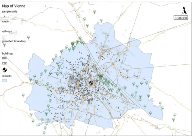
INSERT FIGURE 1

In total, we engage four location variables. Firstly, we include the district in which each apartment unit is located – Vienna has 23 districts within its city limits. When the effects of other structural and location variations are controlled as far as possible within the model, the coefficient of the district variable should show the aggregate positive or negative implicit value associated with the unique characteristics within each district. This is consistent with Baumont (2009) who uses a district variable to demonstrate that houses located in social housing districts are discounted.

In addition to the relative location variable district, we incorporate three variables that measure absolute location of apartment units – distance from the greenbelt, Prater of Vienna and the CBD. First and foremost, distance from the greenbelt is the prime location variable within our enquiry. Vienna has a greenbelt that is located in the outskirts – a green area particularly surrounding the North-West, West, South-West and South-East of the city (see Fig 1). We pin down

10 the border of the greenbelt in order to calculate the shortest distance from the greenbelt to each apartment unit. This variable can capture the amenity value associated with the greenbelt on prices of apartments. The Viennese greenbelt has been an important element of the city landscape at least since 19057; however, it became even more prominent with the Vienna City Council’s approval of the Greenbelt Master plan for a network of green zones and open spaces in 1995 (City of Vienna 2000). Under this policy, not only greenbelt amenities such as forests, national parks, reserves and whole land tracts but also ’green wedges’ such as water bodies and green recreational areas within the city are preserved.

Distance from the Prater of Vienna is included as this is an important urban space within the city. The Prater is a traditional location for a variety of leisure activities including but not limited to the world famous Prater amusement park that provides entertainment particularly for young people and families. Surrounding Danube green areas and the Prater fair grounds elevate the value of these amenities. The new urban setting characterised by the presence of modern trading and service enterprises as well as proposed residential quarters in this area makes this area even more magnetic.

The traditional distance from the CBD variable is included to investigate the proximity effects of the city centre. We consider the 1st district positioned in the heart of the Vienna city to be the CBD and the Stephansdom church located in the middle of the 1st district to be the centre of the CBD. Based on urban economic theory, we should see, ceteris paribus, lower prices of apartments when the distance increases mainly because of weaker accessibility of households to urban infrastructure and services. Table 1 presents above mentioned variables and descriptive statistics.

INSERT TABLE 1

4. Empirical models

The standard hedonic price function is modelled as the following:

= + (1)

where, P is the n × 1 vector of apartment prices, Z is the n × j matrix of explanatory variables,β is the j × 1 vector of coefficients associated with explanatory variables, and ε is the n × 1 vector of independent and identically distributed random error terms. All the variables specified in Table 1 including structural characteristics and location attributes are incorporated within Z above.

7

11 Cross-sectional regression as specified in (1) above is an accurate representation as owner assessed values and apartment characteristics were obtained only over a period of three months. This standard hedonic model is typically estimated using the ordinary least squares (OLS) method.

Location of a dwelling with respect to the greenbelt, the Prater, the CBD and the district, gives a spatial dimension to our data. Thus, in an intra-urban context where observations correspond to apartments close to each other, the spatial autocorrelation arising due to absence of independence between spatial observations is difficult to exclude a priori. Here, spatial autocorrelation is caused by the existence of a relationship between the observed price of an apartment and the prices of other apartments located in its neighbourhood (‘adjacency effect‘; Can 1992) and/or due to omitted variables presenting a spatial configuration within the error structure (Le Gallo 2002). Not taking into account such autocorrelation leads to biased and inconsistent parameter estimates of the hedonic price function. Therefore the presence of spatial autocorrelation needs to be tested and if necessary spatial hedonic methods should be employed.

When testing for spatial autocorrelation and modelling the spatial relationship (and linkage strength) among apartment prices, neighbourhood relationships are taken into account through a spatial weights matrix W. Diagonal elements wii of this matrix are equal to 0 while off-diagonal

elements wij specify how observation i is spatially related to other observations j. This matrix is

exogenously defined, and as it is not possible to know a priori that a certain spatial structure is the most appropriate, six spatial weights matrices are tested. The first 3 matrices are distance-based; (i) WDHALF – all apartments within a circle of 0.5 km of distance to a specific apartment are neighbours to that apartment, (ii) WD1 – all apartments within a circle of 1km of distance to a specific apartment are neighbours, and (iii) WD2 – all apartments within a circle of 2km of distance to a specific apartment are neighbours. The rest of the matrices are based on the k-nearest neighbours; (iv) W1 – the closest (one) apartment to an apartment is the neighbour, (v) W3 – the closest three apartments to an apartment are neighbours, and (vi) W5 – the closest five apartments to an apartment are neighbours.

Spatial weights matrices are row-standardized (W) following the common practice in spatial econometrics (see Franzese and Hays 2008; Anselin 2002; and Anselin and Florax 1995). Row-standardization of spatial weights matrices is typically preferred in order to facilitate the interpretation of underlying models (Tiefelsdorf et al. 1999; Hordijk 1979; and Ord 1975). This ‘standardisation’ means that each element within the matrix is the number of neighbouring elements to a given observation divided by the number of total elements of the matrix. Therefore, use of W matrices also ensures that each row in the matrix adds up to unity (Σj wij = 1), creating a

row-12 stochastic matrix. The W matrix will be asymmetric and its eigenvalues will be less than one in absolute value as a consequence of using row-standardized coding.

Once the presence and possible sources of spatial dependence is known, the hedonic model with a spatial lag term or a spatial error term can be estimated as appropriate in order to take into account this spatial dependence within the model specification.

The spatial lag model (SAR) adds in possible influence of prices of nearby apartments on the price of a given apartment as follows:

= + + (2)

where,

ρ

The spatial error model (SEM), on the other hand, assumes that the error term is spatially dependent. The detection of spatial dependence in the error term reveals a problem of model specification, such as the omission of explanatory variables. Indeed, spatial effects may not be fully captured by the existing explanatory variables and may be reflected in the error term such that:

= +

= + (3)

where, λ is the parameter measuring the strength of spatial autocorrelation within residuals.

The global Moran test is performed in order to test the presence of spatial autocorrelation assuming several different neighbourhood structures as defined above. Test results are presented in Annex 1. Regardless of the spatial weights matrix employed, the null hypothesis is always rejected except one situation where the test is not significant. Since the global Moran test suggests presence of spatial autocorrelation, the choice between the SAR and the SEM is made based on the significance of test results8 of the following Lagrange Multiplier (LM) tests (see Florax et al. 2003):

LMlag test -> H0:ρ = 0 from model (2)

LMerror test -> H0:λ = 0 from model (3)

8

If both LM tests are significant, then Robust LM (RLM) tests are carried out. In both these tests, a higher level of significance of the test statistic indicates the most likely data generation process. See Anselin et al. (1996) for details of these tests.

13 LM tests were carried out for two versions of the model – one with district and the other with distance from the CBD – using the above mentioned six different spatial weights matrices in each case (see Annex 1)9. The results indicate that a SEM should be estimated with respect to 11 out of 12 instances (i.e. 92 % of all cases). Consequently, a SEM is estimated for 11 specifications and SAR for the remaining specification.

Corrado and Fingleton (2011) and Elhorst (2010) recommend that the Spatial Durbin model (SDM) should also be estimated in cases where LM error test or LM lag test is significant. Following this guideline, SDM is estimated for both base models using the spatial weights matrices that produced the best fit spatial error models. The SDM addresses spatial dependence across observations in both the dependent and independent variables in the following form

= + + + (4)

where, θ is the correlation coefficient of the lagged independent variables and all other symbols are as previously defined.

Both the SAR and the SEM are generalised within the SDM. This is because the SDM incorporates within the model specification spillover effects related to explanatory variables that would otherwise have been left in the residuals. As SEM and SDM are estimated by maximum likelihood, a likelihood ratio (LR) test is used to test the hypothesis H0: θ + ρ = 0. This hypothesis tests whether the SDM

can be simplified to the SEM (Elhorst 2010). The LR tests reject the above hypothesis (see annex 2) confirming that the SDM best describes our data.

Interpretation of parameter estimates of the SDM is more complicated as well as richer than the models without spatial lags of the dependent variable or the explanatory variables (Gerkman 2012). Models with spatial lag of the dependent variable require special interpretation of the parameters due to feedback loops and possible influence on all other units in the sample.10 These spillovers between the variables and their spatial lags in the data generating process depicted in SDM thus makes it impossible to compare its results with either the base model or the SEM. Therefore, in order to accurately interpret the coefficients of the SDM, the direct, indirect and total impact estimates of change in variables within the model needs to be examined (LeSage and Pace 2009). The direct impacts occur when a change in a particular explanatory variable of a given unit causes changes in the dependent variable of the same unit, and when such a change can affect the

9

Reasons for using these specifications are detailed in Section 5 (p. 14)

10

14 dependent variable in all units through the feedback effects of spatial lags. On the contrary, when such a change in an explanatory variable of a given unit has an influence on the dependent variables of other units by way of spillovers, then this effect is known as the indirect impact. The combination of both these effects is the total impact. These impacts are averaged over all apartments providing summary measures of direct, indirect and total impacts arising from a change in a particular explanatory variable of a given unit.11

The methods as applied here address the problem of omitted variables while capturing the possible nearby proximity effects (i.e., small-scale neighbourhood). First, omitted variable bias is less of a problem particularly when we include important location variables. For example, Muth (1969), Orford (1999) and Batty and Longley (1987) posit that a property’s structural attributes and its location within the city are related, since they reflect the growth of the urban structure. To further validate this proposition, Cubbin (1970) and Kain and Quigley (1970) have revealed a high degree of multicollinearity between structural attributes and resulting spatial autocorrelation. As we have included four critical location variables, these are expected to incorporate some of the impact of omitted structural variables if any. Second, researchers have more commonly used spatial fixed effect models to address the influence of omitted variables within a spatial context (Beron et al. 2001; Deaton 1988). Variables capturing local fixed effects typically control for neighbourhood characteristics and geographic location in addition to omitted spatial variables. In this paper, we incorporate these fixed effects using a categorical variable for unique districts within Vienna. When omitted variables follow a spatial structure such that the error variance-covariance matrix is no longer diagonal, spatial fixed effects may address this problem at least partly (Anselin and Lozano-Gracia 2008) – however empirical studies have shown this does not resolve the issue completely.

Therefore, we additionally use spatial models that “represent a powerful, underutilized tool in urban and environmental economics, capable of addressing omitted variable bias” (Brasington and Hite 2005, p. 58). The spatial models employed here take into account any spatial linkages and spillover effects and thus are capable of controlling for the unintended consequences of omitted variables that might bias the coefficient on the variable of interest. For example, both property-specific omitted variables as well as those related to neighbouring properties are encompassed in the error term when using a SAR, and the spatial lag term picks up unobserved influences that affect the value of a particular house (Bolduc et al. 1995; Griffith 1988). When omitted variables follow a spatial structure, a SEM captures these effects. The SDM includes lag terms of the dependent variable as

11

Note that the direct impact is represented by the average of diagonal elements of the matrix of partial derivatives, and the indirect effect is represented by the average of off-diagonal elements.

15 well as those of the explanatory variables. Part of the improvement of the spatial Durbin procedure is that it incorporates the influence of omitted variables through the spatially lagged independent variables (Anselin 1988; Pace et al. 1998). The SDM thus captures the influence of all other omitted variables that vary across space at a more localized level – through accounting for possible nearby proximity effects. Collectively, the methods applied here may capture spillovers, omitted variables, or other forms of spatial dependence, and thus are capable of incorporating more influence of omitted variables than the previously used methods.

5. Estimation results

_{and discussion}

Bivariate correlations between the independent variables were examined to assess possible multicollinearity. Based on the general rule of thumb of r > 0.7 (see Tabachnick and Fidell 1996),

number of rooms and living area were found to be correlated. Thus the variable number of rooms

was excluded from the regression models. Also, district and distance from the CBD were found to be correlated. Therefore, two versions of the model were estimated – one with district and the other with distance from the CBD alongside other variables. This path provides two advantages: (i) Models estimated are not prone to multicollinearity, and (ii) Two models facilitate comparison of findings and validate robustness of our conclusions.

The estimation results depend on the functional form of the hedonic models. Its choice has been debated particularly since the seminal paper by Rosen (1974).13 However, the introduction of spatial autocorrelation in the hedonic price function makes it difficult to use the Box-Cox procedure to identify the appropriate functional form.14 As a result, we chose to use the semi-log specification to gain the advantage that coefficient estimates are proportions of the price that are directly attributable to the respective characteristics. In cases where predictors are ratio (and hence log-transformed) variables, however, parameter estimates are interpreted as elasticities. Use of log form for ratio variables and the linear form for categorical variables offers an accurate econometric exercise as well as a better interpretation of our parameter estimates.

Once spatial autocorrelation was detected, the most appropriate spatial specifications were determined based on the LM test results. Superior models in terms of estimation performance were chosen for comparison using the Akaike information criteria (AIC). AIC is a commonly used measure of overall model performance that takes into account also the model complexity in the context of

12

The analysis was performed using the spatial statistics software R (R Development Core Team, 2011).

13

See Cropper et al. (1988) for a discussion on this topic.

14

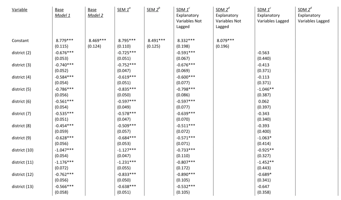
16 non-nested models (Jones et al. 2003). The best performing SEM with the variable district uses a 2 km distance threshold as the neighbourhood criteria while the best performing spatial model with the variable distance from the CBD uses a 1 km distance threshold. Results of the two versions of the preliminary hedonic model and the best fit spatial models are presented in Table 2.15 These reported estimations are as follows: Base Model 1 – Non-spatial hedonic model with district; Base Model 2 – Non-spatial hedonic model with distance from the CBD; SEM 1 – Spatial error model with district; SEM 2 – Spatial error model with distance from the CBD; SDM 1 – Spatial Durbin model with district; SDM 2 – Spatial Durbin model with distance from the CBD.

The studentized Breusch-Pagen test was performed to check the reliability of the tests for spatial effects. The results indicate presence of heteroscedasticity (see Table 2). However, as Kelejian and Robinson (2004) have demonstrated, the tests for spatial effects are robust as far as it is not spatially correlated. Therefore, these tests of spatial effects can be considered reliable in the context of our study.

INSERT TABLE 2

Estimates obtained for intrinsic characteristics are of the expected sign and generally consistent across the six models. An increase in living area, position on the top floor, presence of a balcony, terrace, elevator, basement and parquet flooring all add positively to the apartment value. In addition, better quality of an apartment has a positive impact on price: those rated as ‘moderate’ by the owners have lower values compared to ‘best’ condition apartments and, ‘bad’ condition reduces price by even a larger amount. Apartments on the fourth floor and above and particularly those on the top floor attract a premium. This premium sequentially increases with the floor level affirming the premium attached to a ‘view’ documented in the literature (see Benson et al. 1998; Bastian et al. 2002; and Paterson and Boyle 2002). A finding that is difficult to explain based on theory is the negative coefficient associated with an increase from one toilet to two, two toilets to three and one bath to two. This is possibly a result of excluding apartments with more than seven rooms to contain a homogeneous sample of apartments.16 Direction and the magnitude of parameter estimates of variables size (living area) and good condition in Feilmayr’s (2004) study is very similar to those in the present study.

15

Other spatial models tested using alternative spatial weights matrices are not shown due to space reasons, and available on request.

16

Having more than one toilet or bath in a small apartment does not necessarily increase its value (one toilet or bath is feasibly adequate for a small apartment and adding more could impose a maintenance burden): higher maintenance costs translate into lower apartment price.

17 The included extrinsic characteristics also influence prices of apartments. Firstly, as the reference district here is the 1st district – the CBD – a negative coefficient related to other districts highlights that moving away from the CBD depresses apartment price. This prominence of districts in explaining Viennese rents is acknowledged in Brunauer et al (2009). Additionally, Herath and Maier (2013) demonstrate that a negative effect on prices related to districts other than the CBD can result from differences in neighbourhood characteristics including amenities such as recreation facilities, access to public transport and service centres, social composition and other conditions such as demand determinants. Our findings thus confirm that the CBD composes a desired bundle of amenities within the city. This significance of districts could be further explained referring to the geography of Vienna where specific districts are distributed in the following way: the 1st district is the CBD (inner ring); the closest districts to the CBD are just outside the inner ring (districts 2 to 9); and the rest of the districts (districts 10 to 23) are in the outskirts. Due to this concentric urban structure of the city of Vienna, the density of public services including access to the transport network is likely higher in the CBD. Similarly, concentration of these facilities within districts 2 to 9 is likely higher than in districts 10 to 23. Findings of the study completed by Wieser (2006) support this radial transport network argument with reference to Vienna.

Distance from the CBD is an absolute measure of location compared to the relative measure

of location district. In models where the variable distance from the CBD is employed, the coefficient of this variable is negative and highly significant. Consistent with the rent gradient hypothesis, this finding across models empirically demonstrates that the apartment units further away from the CBD have a lower price. This also suggests if two units are located at the same distance from the CBD but in two different districts, all else constant, then differences of amenities in two districts will determine the variation of prices.

Noteworthy are the findings highlighting the role of green amenities in the formation of apartment prices. First, distance from the greenbelt has the expected negative coefficient in both base models as well as spatial error models. This result is similar to those obtained by for instance Morancho (2003) and Nelson (1988). In the base model with district, the dimension of the negative coefficient is small and significant at the 1% level whereas in the alternative base model (i.e. model with distance from the CBD) not only that the dimension of the coefficient has improved substantially, the significance level has also increased to the 0.1% level. Also, both models fit well in terms of explanatory power and the overall model performance.

Additionally, our results strongly suggest that urban green areas are preferred by the Viennese homebuyers. The estimated parameter for the variable distance from the Prater depicts

18 that the aesthetic value brought in by the amusement park, Danube green areas and the Prater fair grounds have an influence on apartment prices. This urban space variable shows a larger negative impact on price in the base models as well as spatial error models with district as the location variable over the same models with distance from the CBD.

As mentioned in Section 4, a significant model improvement can be achieved through the SDM. Base model estimates are biased and inconsistent since the λ parameter of the SEM and the ρ parameter of the SDM are significant in our results. In addition, a comparison of estimated coefficients from the base model and SDM confirms there is an upward bias in the base model parameters. This is in line with the theoretical argument that non spatial models produce larger estimates since they tend to attribute variation in the dependent variable to the explanatory variables that would otherwise be attributed to the spatial lag of the dependent variable.

In addition to LR tests suggesting improved performance of the SDM, the ρ parameter in the SDM is stable across alternative models (see Table 3). In contrast, λ parameters of the SEM results are unstable. The positive spatial autocorrelation and highly significant errors in the SEM 2 (λ = 0.70) can be demonstrated as a positive spatial diffusion effect among real estate prices (Baumont and Legros 2009). On the contrary, SEM 1 suggests a negative spatial error autocorrelation (λ = -0.75). This difference in terms of λ parameter is possible given on the one hand, these two models include different location variables – district and distance from the CBD. On the other hand, the best performing SEM 1 includes all apartments located within 1 km distance from a given apartment as neighbours compared to a 2 km threshold in the SEM 2.

The direct and total impact estimates calculated for the SDM estimation exhibit similar dimensions and directions of effects to those produced by the base model and the SEM estimations (see Table 3). Consequently, structural attributes living area, top floor, presence of balcony, terrace, elevator, basement and parquet flooring have a positive influence on apartment prices.17 The negative effect of bad and moderate condition compared to best condition of an apartment on price is further validated through SDM findings. Larger negative impact of bad condition relative to moderate condition is also substantiated. The findings of the SDM thus confirm the previous findings from both the base model and the SEM.

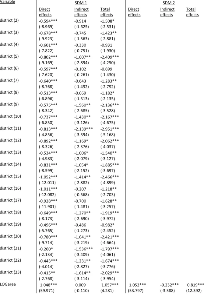
INSERT TABLE 3

17

Note in the case of elevator, the direct impact shows this positive effect on price (this is to state that an apartment’s own elevator have an impact on price).

19 Nevertheless, SDM impact estimates demonstrate that unlike shown in the base model and SEM results, some of the impacts that arise from these explanatory variables are actually related to spillover effects. As these spillovers result from the other apartments in the sample, this could be explained as a neighbourhood effect. One such example is found in the context of the variable bad

condition. While the direct negative impact of this variable is related to an apartment’s own bad

condition, the negative and significant indirect impact points to a negative spillover effect. In other words, an apartment with bad condition negatively affects the value of neighbouring apartments. This way, SDM impact estimates can explain important characteristics of the close neighbourhood.

The parameter estimates produced by the SDM are superior to those produced by the base model, SAR and the SEM as the former accounts for feedback loops that exist among dependent and explanatory variables as well as spillover effects. The impact estimates calculated for each district in SDM 1 validate the negative impact of location in districts other than the CBD on apartment price. While most of the district variables indicate significant direct impacts, several districts also show significant indirect impacts suggesting spillover effects associated with location of other apartments in these districts. Nevertheless, the CBD stands out as containing a desired bundle of amenities within Vienna supporting the theoretical arguments related to urban amenities theory.

The variable distance from the CBD in SDM 2 demonstrates a negative and significant impact on price of apartments. The effect of this variable on apartment prices is exclusively a direct impact providing no evidence of any spillover effects. In addition to supporting the understanding of a circular city structure and radial transport network, this finding substantiates the significance of the CBD as an economic, recreational and touristic centre of the city.

The variable distance from the greenbelt in SDM 1 has a positive and significant direct impact although the total impact is negative. This is due to the fact that negative indirect impact surpasses the positive direct impact. SDM 2 also highlights this negative and significant indirect impact as well as the negative total impact. Both these results imply that the impact of distance from the greenbelt on price is mainly caused by indirect effects generated by spillovers. In other words, the price of an apartment is lower when its neighbouring apartments are located further from the greenbelt. However, distances between neighbouring apartments are small within our sample given the neighbourhood criteria adopted. Therefore, this outcome reiterates the same negative relation between distance from the greenbelt and apartment price. Drilling down more, the base model demonstrates that the price of a constant-quality apartment is found to decline by approximately 0.04-0.15% (depending on the specification) with every 1% increase in distance from the greenbelt. The corresponding decline of price in the SEM is 0.04-0.06% revealing an upward bias in the base

20 model estimation. Overall, despite these minor differences in the parameter estimates, the results of the base model, SEM and, more importantly, the SDM which is considered to be superior all support a negative rent gradient when moving away from the greenbelt.

In addition, apartment prices are partly explained by distance from the Prater. The SDM 1 produces a negative and significant direct impact for this variable, and the total impact is also negative but insignificant. This negative impact is possibly generated by, on the one hand, the recreational value of this site that is created by the amusement park. On the other hand, the environmental and aesthetic value of Danube green areas and the Prater fair grounds likely contribute to this as well. There is a negative total impact in SDM 2 for this variable although not significant.

Overall, the distance from the CBD variable has a significant and a larger impact on apartment prices compared to the variables distance from the greenbelt and distance from the

Prater. This finding is consistent across the base model as well as spatial model specifications. More

importantly, the superior SDM also demonstrates that this negative impact on apartment price is formed by the direct effects of distance from the CBD variable rather than any spillovers present in the system. These findings empirically corroborate the idea that proximity to the greenbelt and urban green areas are also important although proximity to the CBD is the most significant location-related predictor in the context of the Viennese apartment prices.

6. Conclusion

In a world where costs involved in providing amenities to the public are known and precise benefits of such amenities are relatively unknown, hedonic price method could be employed to assess the optimal level of production of these public goods taking into account individual preferences. Such analyses can guide urban planning in terms of setting priorities for public action. The purpose of this article was to examine the impact of proximity to the greenbelt on apartment prices in the city of Vienna with the intention of developing an understanding of demand for this amenity. In order to ascertain the pure effect of greenbelt on apartment prices, a number of structural variables and other location variables were employed as control variables.

Findings of this study provide evidence of benefits of the greenbelt as well as urban green spaces. The variables distance from the greenbelt and distance from the Prater are negatively related to apartment price, and the results of the spatial Durbin Model substantiate these findings. Our results clearly show that the proximity to the greenbelt partly explains the apartment prices. In

21 addition, proximity to the urban green areas Prater and Danube also induces an increase of apartment price. The premium attached to the greenbelt is slightly larger than that of the urban green area. These results show the important role of green amenities in residential choice of households. The benefits of living in proximity to these green amenities, however, are estimated to be not as important as those related to living close to the CBD. In that respect, our study sheds light on how the trade-off between proximity to the city centre and the green area is negotiated by home-buyers.

There is a clear research implication of undertaking the spatial analysis. First, this methodology is in line with the strong theoretical arguments available against non-spatial hedonic models due to biased and inefficient parameter estimates they produce, and in favour of spatial hedonic models due to more robust parameter estimates. If spatial analysis provides different results than non-spatial analysis, this shows that reliance on traditional non-spatial hedonic methods may lead to flawed conclusions concerning the spatial structure of the price function. Since values of green amenities are typically examined in non-spatial settings, spatial analysis can validate findings of non-spatial analysis and also indicate the spatial relation among neighbours in the empirical context. Most importantly, spatial models address the well documented problem of omitted variable bias.

Our results indicate that provision of a greenbelt can be vital for the development of a city whose control is the prerogative of local policy makers. Indeed, in the context of competitive territorial management, green amenities are an approach to development and differentiation of a city through the promotion of a pleasant living environment to meet the growing sensitivity of populations to sustainable development and environmental conservation. Similarly, it can facilitate harmonising of different neighbourhoods within a city, by contributing to an improvement in deprived areas. As shown in this article, the important role of the greenbelt as an amenity leads to more complex public decision making in the setting of urban development. These concerns can be addressed through a further enquiry into understanding perceptions of the households in the city of Vienna on the usefulness of the greenbelt and how it is valued. In that way, the implementation of alternative environmental valuation methods such as the contingent valuation method or choice experiments could usefully supplement the results obtained in this study.

22

References

Abbasi SA, Khan FI (2000) Greenbelts for Pollution Abatement: Concepts, Design, Applications, Discovery Publishing House, MI.

Amati M, Yokohari M (2006) Temporal changes and local variations in the functions of London's green belt. Landscape and Urban Planning. 75, 125-142.

Anselin L (1988) Spatial Econometrics: Methods and Models, Kluwer, Dordrecht.

Anselin L (2002) Under the hood: issues in the specification and interpretation of spatial regression models. Agricultural Economics. 27(3), 247-267.

Anselin L, Bera A, Florax RJGM, Yoon M (1996) Simple diagnostic tests for spatial dependence. Regional Science and Urban Economics. 26, 77-104.

Anselin L, Florax RJGM (1995) Small sample properties of tests for spatial dependence in regression models: some further results, in: Anselin, L., Florax, R.J.G.M. (Eds.), New Directions in Spatial Econometrics. Springer, Berlin, pp. 21-74.

Bastian CT, McLeod DM, Germino MJ, Reiners WA, Blasko BJ (2002) Environmental amenities and agricultural land values: a hedonic model using geographic information systems data. Ecological Economics. 40, 337-349.

Baumont C, Legros D (2009) Neighborhood effects in spatial housing value models: the case of the metropolitan area of Paris (1999). Document de travail du Laboratoire d'Economie et de Gestion, No. e2009-09, Université de Bourgogne.

Baumont C (2009) Spatial effects of urban public policies on housing values. Papers in Regional Science. 88(2), 301-326.

Bengston DN, Youn YC (2006) Urban containment policies and the protection of natural areas: the case of Seoul's greenbelt. Ecology and Society. 11(1): 3. [online] URL: http://www.ecologyandsociety.org/vol11/iss1/art3/

Benson ED, Hansen JL, Schwartz AL, Smersh GT (1998) Pricing residential amenities: the value of a view. Journal of Real Estate Finance and Economics. 16(1), 55-73.

Bolund P, Hunhammar S (1999) Ecosystem services in urban areas, Ecological Economics. 29(2), 293-301.

Brander LM, Koetse MJ (2011) The value of urban open space: meta-analyses of contingent valuation and hedonic pricing results. Journal of Environmental Management. 92, 2763-2773.

Brunauer WA, Lang S, Wechselberger P, Bienert S (2009) Additive hedonic regression models with spatial scaling factors: an application for rents in Vienna. Journal of Real Estate Finance and Economics. 41(4), 390-411.

Bullock CH (2008) Valuing urban green space: hypothetical alternatives and the status quo. Journal of Environmental Planning and Management. 51, 15-35.

23 Can A (1992) Specification and estimation of hedonic price models. Regional Science and Urban Economics. 22, 453-474.

Cheshire P, Sheppard S (1989) British planning policy and access to housing: some empirical estimates. Urban Studies. 26, 469-485.

Choumert J, Salanié J (2008) Provision of urban green spaces: some insights from economics. Landscape Research. 33, 331-345.

City of Vienna (2000) Strategy Plan for Vienna - Summary. Municipal Department for Urban Development and Planning, Vienna, Austria.

Corrado L, Fingleton B (2011) Where is the economics in spatial econometrics, SERC Discussion Paper 71.

Correll MR, Lillydahl JH, Singell LD (1978) The effects of greenbelts on residential property values: some findings on the political economy of open space. Land Economics. 54(2), 207-217.

Crompton JL (2000) The impact of parks and open space on property values and the property tax base. National Recreation and Park Association, Ashburn, Virginia.

Crompton JL, Love LL and More TA (1997) An empirical study of the role of recreation, parks and open space in companies' (re)location decisions. Journal of Park and Recreation Administration. 15(1), 37-58.

Cropper ML, Deck LB, McConnell KE (1988) On the choice of funtional form for hedonic price functions. The Review of Economics and Statistics. 70(4), 668-675.

De Vries S, Verheij RA, Groenewegen PP, Spreeuwenberg P (2003) Natural environments - healthy environments? An exploratory analysis of the relationship between greenspace and health. Environment and Planning A. 35(10), 1717-1731.

Dwyer JF, Peterson GL, Darragh AJ (1983) Estimating the value of urban forests using the travel cost method. Journal of Arboriculture. 9(7), 182-185.

Elhorst JP (2010) Applied spatial econometrics: raising the bar. Spatial Economic Analysis. 5(1), 9-28. Fausold CF, Lilieholm RJ (1999) The economic value of open space: a review and synthesis, Environmental Management. 23 (3), 307-320.

Feilmayr W (2004) Immobilienindizes aus Hedonischen Regressionen, in: Seminarbericht 47, Seminarbericht der Gesellschaft für Regionalforschung, Gesellschaft für Regionalforschung, Heidelberg, pp. 74-98.

Florax RJGM, Folmer H, Rey SJ (2003) Specification searches in spatial econometrics: the relevance of Hendry's Methodology. Regional Science and Urban Economics. 33, 557-579.

Franzese R, Hays JC (2008) Spatial-Econometric Models of Interdependence. Book prospectus.

Garrod G, Willis K (1992) The environmental economic impact of woodland: a two-stage hedonic price model of the amenity value of forestry in Britain. Applied Economics. 24, 715-728.

24 Gerkman L (2012) Empirical spatial econometric modelling of small scale neighbourhood. Journal of Geographical Systems. 14(3), 283-298.

Hanley N, Knight J (1992) Valuing the environment: recent UK experience and an application to green belt land. Journal of Environmental Planning and Management. 35(2), 145-160.

Henneberry J (1998) Transport investment and house prices. Journal of Property Valuation and Investment. 16(2), 144-158.

Herath S, Maier G (2013) Local particularities or distance gradient — what matters most in the case of the Viennese apartment market?. Journal of European Real Estate Research. 6(2).

Hordijk L (1979) Problems in estimating econometric relationships in space. Papers of the Regional Science Association. 42, 99-115.

Jim CY, Chen WY (2008) Assessing the ecosystem service of air pollution removal by urban vegetation in Guangzhou (China). Journal of Environmental Management. 88(4), 665-676.

Jo H-K, McPherson GE (1995) Carbon storage and flux in urban residential greenspace. Journal of Environmental Management. 45(2), 109-133.

Jones C, Leishman C, Watkind C (2003) Structural change in a local urban housing market, Environment and Planning. 35(7), 1315-1326.

Kadish J, Netusil NR (2012) Valuing vegetation in an urban watershed. Landscape and Urban Planning. 104(1), 59-65.

Kelejian HH, Robinson DP (2004) The influence of spatially correlated heteroskedasticity on tests for spatial correlation, in: Anselin, L., Florax, R.J.G.M., Rey, S.J. (Eds.), Advances in Spatial Econometrics: Methodology, Tools and Applications. Springer, pp. 79-97.

Kuhn M (2003) Greenbelt and green heart: separating and integrating landscapes in European city regions. Landscape and Urban Planning. 64, 19-27.

Kuo FE, Sullivan WC (2001) Aggression and violence in the inner city: effects of environment via mental fatigue. Environment and Behavior. 33(4), 543-571.

Le Gallo J (2002) Econométrie spatiale : l'autocorrélation spatiale dans les modèles de régression linéaire. Economie et Prévision. 155, 139-157.

Le Goffe P (2000) Hedonic pricing of agriculture and forestry externalities. Environmental and Resource Economics. 15, 397-401.

Lee C-M, Linneman P (1998) Dynamics of the greenbelt amenity effect on the land market - the case of Seoul's greenbelt. Real Estate Economics. 26(1), 107-129.

LeSage JP, Pace RK (2009) Introduction to Spatial Econometrics, Taylor & Francis, Boca Raton.

Maas J, van Dillen SME, Verheij RA, Groenewegen PP (2009) Social contacts as a possible mechanism behind the relation between green space and health. Health & Place. 15(2), 586-595.

25 Maas J, Verheij RA, Groenewegen PP, de Vries S, Spreeuwenberg P (2006) Green space, urbanity, and health: how strong is the relation? Journal of Epidemiology and Community Health. 60(7), 587-592. McConnell V, Walls M (2005) The value of open space: evidence from studies of nonmarket benefits. Resources for the Future, Washington, D.C.

Melichar J, Kaprová K (2013) Revealing preferences of Prague's homebuyers toward greenery amenities: the empirical evidence of distance-size effect. Landscape and Urban Planning. 109, 56-66. Morancho AB (2003) A hedonic valuation of urban green areas. Landscape and Urban Planning. 66, 35-41.

Nelson AC (1985) A unifying view of greenbelt influences on regional land values and implications for regional planning policy. Growth and Change. 16(2), 43-48.

Nelson AC (1988) An empirical note on how regional urban containment policy influences an interaction between greenbelt and exurban land markets. Journal of the American Planning Association. 54 (2), 178-184.

Ord JK (1975) Estimation methods for models of spatial interaction. Journal of the American Statistical Association. 70, 120-126.

Orford S (1999) Valuing the Built Environment: GIS and House Price Analysis, Aldershot, Ashgate. Pandit R, Polyakov M, Tapsuwan S, Moran T (2013) The effect of street trees on property value in Perth, Western Australia. Landscape and Urban Planning. 110, 134-142.

Paterson RW, Boyle KJ (2002) Out of sight, out of mind? Using GIS to incorporate visibility in hedonic property value models. Land Economics. 78(3), 417-425.

Pendall R, Martin J (2002) Holding the line: urban containment in the United States, Discussion Paper Prepared for The Brookings Institution Center on Urban and Metropolitan Policy.

Prow T (1999) The power of trees. The Illinois Steward Magazine. 7(4).

R Development Core Team (2011) R: A Language and Environment for Statistical Computing, Vienna, Austria: R Foundation for Statistical Computing.

Rambonilaza M (2004) Evaluation de la demande de paysage : Etat des lieux et réflexions sur le transfert des valeurs disponibles. Cahiers d'Economie et Sociologie Rurales. 70,70-101.

Rosen S (1974) Hedonic prices and implicit markets: product differentiation in pure competition. Journal of Political Economy. 82, 34-55.

Sander HA, Haight RG (2012) Estimating the economic value of cultural ecosystem services in an urbanizing area using hedonic pricing. Journal of Environmental Management. 113, 194-205.

Tabachnick BG, Fidell LS (1996) Using Multivariate Statistics, New York: Harper Collins.

Tiefelsdorf M, Griffith DA, Boots BA (1999) A variance stabilizing coding scheme for spatial link matrices. Environment and Planning A. 31, 165-180.

26 Tyrvainen L (1997) The amenity value of the urban forest: an application of the hedonic pricing method. Landscape and Urban Planning. 37, 211-222.

Tyrväinen L, Miettinen A (2000) Property prices and urban forest amenities. Journal of Environmental Economics and Management. 39, 205.223.

Tzoulas K, Korpela K, Venn S, Yli-Pelkonen V, Kazmierczak A, Niemela J, James P (2007) Promoting ecosystem and human health in urban areas using green infrastructure : a literature review. Landscape and Urban Planning. 81(3), 167-178.

Waltert F, Schläpfer F (2010) The role of landscape amenities in regional development: a survey of migration, regional economic and hedonic pricing studies. Ecological Economics. 70, 141-152.

Wieser R (2006) Hedonic prices on Vienna's urban residential land markets. Working Paper Nr.: 2/2006. Centre of Public Finance and Infrastructure Policy, TU Wien, Vienna, July.

Willis KG, Whitby MC (1985) The value of green belt land. Journal of Rural Studies. 1(2), 147-162. Willis K, Osman L (2005) Economic benefits of accessible green spaces for physical and mental health: scoping study. Forestry Commission, CJC Consulting, Oxford.

Witt PA, Crompton JL (1996) The at-risk youth recreation project. Journal of Parks and Recreation Administration. 14(3), 1-9.

Zhang L, Liu Q, Hall, NW, Fu Z (2007) An environmental accounting framework applied to green space ecosystem planning for small towns in China as a case study. Ecological Economics. 60(3), 533-542.

INSERT ANNEX 1 INSERT ANNEX 2

27 Fig 1. The greenbelt boundary and the CBD with the sample apartment units within the city of Vienna.