-1
Research Article
The importance of spatial scale in habitat models: capercaillie in the Swiss Alps
Roland F. Graf
1,2,*, Kurt Bollmann
1, Werner Suter
1and Harald Bugmann
2 1Swiss Federal Research Institute WSL, Zu¨rcherstrasse 111, CH-8903 Birmensdorf, Switzerland; 2Forest Ecology, Department of Environmental Sciences, Swiss Federal Institute of Technology Zu¨rich ETH, CH-8092 Zu¨rich, Switzerland; *Author for correspondence (e-mail: [email protected])
Received 18 June 2004; accepted in revised form 3 January 2005
Key words:Conservation, Landscape analysis, Logistic regression, Multi-scale habitat model, Spatial scale, Switzerland, Tetrao urogallus
Abstract
The role of scale in ecology is widely recognized as being of vital importance for understanding ecological patterns and processes. The capercaillie (Tetrao urogallus) is a forest grouse species with large spatial requirements and highly specialized habitat preferences. Habitat models at the forest stand scale can only partly explain capercaillie occurrence, and some studies at the landscape scale have emphasized the role of large-scale effects. We hypothesized that both the ability of single variables and multivariate models to explain capercaillie occurrence would vary with the spatial scale of the analysis. To test this hypothesis, we varied the grain size of our analysis from 1 to just over 1100 hectares and built univariate and multivariate habitat suitability models for capercaillie in the Swiss Alps. The variance explained by the univariate models was found to vary among the predictors and with spatial scale. Within the multivariate models, the best single-scale model (using all predictor variables at the same scale) worked at a scale equivalent to a small annual home range. The multi-scale model, in which each predictor variable was entered at the scale at which it had performed best in the univariate model, did slightly better than the best single-scale model. Our results confirm that habitat variables should be included at different spatial scales when species-habitat relationships are investigated.
Introduction
Wildlife research and management have tradi-tionally focused on small spatial scales. More recently, it has been recognized that animals, particularly birds, also respond to habitat factors at coarser spatial scales (Freemark and Merriam 1986). Because each species responds to the environment at a unique range of scales (Levin 1992), there is no single correct spatial scale at which to describe species-habitat relationships (Wiens 1989). Thus, multi-scale approaches are necessary (Bissonette 1997; Cushman and
McGarigal 2004) and are indeed becoming more and more common in studies of species-habitat relationships (Carroll et al. 1999; Fuhlendorf et al. 2002; Lawler and Edwards 2002; Thompson and McGarigal 2002; Zabel et al. 2003; Fischer et al. 2004). Many studies, however, are con-ducted at a few arbitrary chosen scales (e.g. Zabel et al. 2003; Johnson et al. 2004), only few include a discrete range of scales (Fuhlendorf et al. 2002; Lawler and Edwards 2002), and very few investigate species-habitat relationships along a continuous range of scales (Thompson and McGarigal 2002).
The rapidly advancing GIS-technology and new powerful statistical tools have helped to address spatial scale questions in species-habitat relation-ships (Guisan and Zimmermann 2000; Manly et al. 2002). Generalized linear models (GLM) are one of the most widespread statistical approaches in habitat modeling (e.g. Mladenoff and Sickley 1998; Sachot et al. 2003; Gibson et al. 2004). As they do not require response variables that are normally distributed, and since they allow non-constant variance functions to be modeled, they are more flexible than the classical least-square regression (Guisan and Zimmermann 2000). A special case of GLM is the logistic regression, where the response variable is dichotomous (Hosmer and Lemeshow 1989; Manly et al. 2002). As data on species dis-tributions are often restricted to the information of presence–absence, logistic regression is extensively used in habitat modeling of various taxonomic groups (Mladenoff and Sickley 1998; Carroll et al. 1999; Mace et al. 1999; MacFaden and Capen 2002; Berg et al. 2004; Gibson et al. 2004).
An excellent model organism for investigating the importance of spatial scale in habitat selection is the capercaillie (Tetrao urogallus, Tetraonidae, Aves; Storch 1997). This large forest grouse species has specialized habitat preferences (e.g. Schroth 1992; Sjo¨berg 1996) and extensive spatial require-ments (average home range: ca. 550 ha, Storch 1995), both making it highly susceptible to habitat and landscape changes. Capercaillie populations are declining in most of their central European range (e.g. Klaus et al. 1986; Storch 2000a), as loss and fragmentation of suitable habitats have split populations into smaller units loosely connected or even completely isolated. This is especially true in Switzerland, where the remaining population of 900–1000 individuals (Mollet et al. 2003) faces a high risk to become extinct due to environmental, demographic, and genetic processes.
In capercaillie, most research as well as conser-vation measures so far have focused on the forest stand scale (e.g. Klaus et al. 1985; Schroth 1992). Telemetry studies in Scandinavia and in Central Europe have revealed that spatial requirements of capercaillie are extensive (Wegge and Larsen 1987; Storch 1995), and they have shown that caper-caillie populations are also sensitive to the spatial configuration of preferred habitats and to forest fragmentation (Rolstad and Wegge 1989). Recent work showed that capercaillie populations are
strongly driven by landscape-scale processes (Storch 1997; Kurki et al. 2000). These processes, however, have only partly been addressed in pre-dictive habitat modeling designed for large spatial scales. The habitat models for capercaillie at the landscape scale that are presently available either do not address spatial scale explicitly (Sachot et al. 2003), do not include spatial variables (Storch 2002) or do not include different spatial scales in a single statistical model (Suchant 2002). Uncover-ing larger-scale habitat relationships is an impor-tant research need in those regions where the species is endangered (Storch 2000b), and analyses should be conducted at multiple scales (Keppie and Kierstead 2003).
In the present study, we analyzed the species-habitat relationships of capercaillie at different spatial scales by varying the grain size. We hypothesized that the predictive power of single variables would vary with the spatial scale of analysis so that an optimum scale could be deter-mined for each predictor variable. Therefore, we expected multi-scale models (every variable entered at its best-explaining scale) to perform better than single-scale models where all variables are entered at the same scale. To test this hypothesis, we built univariate and multivariate habitat suitability models using presence–absence data of capercaillie in the Swiss Pre-Alps and Alps and a large set of environmental predictors.
Methods Study area
The study area comprises 4500 km2 of forest-dominated landscape within the northern Pre-Alps and the eastern Central Alps in Switzerland, ranging in altitude from 400 to 3500 m a.s.l. (Figure 1). The upper tree line on average is at about 2000 m a.s.l. Deciduous trees (mostly beech Fagus sylvatica) dominate the forests in the lower zones (400–1000 m a.s.l.), mixed forests prevail at intermediate altitudes (800–1400 m a.s.l.), and conifer trees such as silver fir (Abies alba), norway spruce (Picea abies) and mountain pine (Pinus mugo) form the forests at higher altitudes (1200–2200 m a.s.l., Steiger 1994).
In the Swiss Alps, capercaillie inhabit conifer-dominated forests at altitudes of about
1000–2200 m a.s.l. Most of the capercaillie popu-lations in the northern Pre-Alps (comprising ca. 280 individuals) and about half of the populations of the eastern Central Alps (comprising ca. 180 individuals) are included within the study area. Particularly in the northern Pre-Alps, capercaillie abundance has decreased strongly in the past decades (Mollet et al. 2003). Loss of suitable habitat, human disturbance and increasing pred-ator abundance are generally thought to be the major reasons.
Modeling design
Presence–absence data and environmental vari-ables were processed in grid format with a cell size of 1 ha. We defined cells as ‘presence’ if they contained at least one capercaillie record. These records came from our own fieldwork and from several regional inventories. They include sightings and indirect evidence of capercaillie presence (faeces, feathers, footprints, etc.). Not all presence cells were used in the analyses, as their clumped distribution could have led to autocorrelation problems. Therefore, we reduced the number of cells by applying thiessen polygons (ARC/INFO 8.3), so that the minimum distance between any two presence cells was at least 500 m.
As the records are mainly from winter and spring surveys the areas with observations can be interpreted as core areas of capercaillie distribu-tion. In late winter and early spring, capercaillie
concentrate near the leks. Summer and autumn ranges contain the winter and spring ranges but also additional areas close to the winter ranges (Hess, pers. comm.). Therefore, we placed a buffer of 1 km around all observations to include the winter and summer ranges to a large degree. This leads to a minimum buffer area of about 3 km2, which equals about the size of the home range of a capercaillie individual, as home range size in telemetry studies ranged from 1 km2(only summer home range, Rolstad et al. 1988) up to 5.5 km2 (Storch 1995). Using this method, we also avoid that actual presence cells (where no record was obtained) are erroneously classified as absence.
Absence cells used in the analysis are a ran-domly selected subset of cells with a minimum distance of 500 m. They additionally have a minimum distance of 1 km and a maximum distance of 5 km to the next presence cell. The latter rule ensured that only those areas are in-cluded that are located within a realistic dis-persal distance from actual capercaillie populations (Storch and Segelbacher 2000; Segelbacher et al. 2003). By doing so, we implicitly assume habitat suitability to be the reason for the absence of capercaillie, not large-scale population effects.
Since both presence and absence cells tend to show a clumped distribution, spatial autocorrelation has to be considered. If autocor-relation was a problem, one would expect the residuals from the fitted models to be spatially correlated (Augustin et al. 1996). We investigated
Figure 1. Study area; the study regions do not contain the whole capercaillie distribution in Switzerland; the dashed line separates the two regions of the northern Pre-Alps and the eastern Central Alps.
the spatial dependence of the residuals of all the multivariate models by calculating Moran’s I (Moran 1948) in the software R 1.7.1. (package: spatial dependence SPDEP) at the level of the first neighbor. Another alternative would have been to account for spatial autocorrelation in the models by including an extra covariate describing whether the species is present or absent in the neighbor-hood of a site (Smith 1994; Augustin et al. 1996). However, this would have made it impossible to apply the models in areas where capercaillie distribution was mapped incompletely.
Environmental variables
A large set of environmental parameters that could possibly influence capercaillie occurrence, and which were available area-wide for the whole country were used as independent variables (Table 1). The 30 variables express aspects of
topography, climate, habitat and human distur-bance.
Topography is supposed to influence the habitat quality of capercaillie, for instance, indirectly by influencing forest structure (Roth and Niever-gelt 1975; Suchant 2002) or directly by affecting the ability of capercaillie to avoid predators. As parameters representing different aspects of topography, we used altitude, slope (steepness) and topographic position. The topographic posi-tion is a measure to express the exposure of a location in space compared to the surrounding terrain. Positive values express relative ridges, hilltops and exposed sites, negative values, on the other hand, stand for sinks, gullies, valleys or toe slopes. The topographic position was calculated in GIS by applying circular moving-windows with increasing radii to a digital elevation model (DEM; DHM25 Ó 2004, SWISSTOPO, DV033594; (Zimmermann and Roberts 2001).
Table 1. Environmental variables.
Variable description Abbreviation Unit (range) Dropped because of correlation (rS> 0.5) with
Altitude DEM m TAVE
Slope (steepness) SLOPE degrees
Topographic position TOP Unitless
Potential direct solar radiation in April SDIR kJ/day Precipitation (June) PREC 0.1 mm/month Average temperature (June) TAVE °C*100 Proportion of forest PFOR %*4 (0–25) Density of forest edges FE %*4 (0–25)
Distance to forest edges DFE m
Forest type FT Four categories FTC
Coniferous forest ratio CFR Index FTC
Proportion of coniferous forest (cat. 1 and 2) CF %*6.25 (0–16) PFOR Coniferous forest (cat. 1 and 2) FTC 0/1
Deciduous forest (cat. 3 and 4) FTD 0/1 TAVE Proportion of mires and wet forests MIRE %*4 (0–25)
Distance to mires and wet forests DMIRE m
Total density of roads and trails (cat. 1–6) RO m/ha TAVE Density of motorable roads (cat. 1–4) ROD m/ha TAVE
Distance to roads and trails DRO m DROD
Distance to motorable roads DROD m Distance to alpine ski runs DSKI m
Density of settlements SETTL 0/1 TAVE
Distance to settlements DSETTL m DROD
Distance to farmland used all year DAGRY m DROD Distance to farmland used seasonally DAGRS m TAVE
Distance to farmland DAGR m PFOR
Proportion of farmland AG %*4 (0–25) TAVE
Proportion of farmland used all year AGY %*4 (0–25)
Local climate is an important factor affecting reproduction of capercaillie, with dry and warm weather in early summer reducing chick mortality (Moss et al. 2001). We used average temperature, precipitation and potential direct solar radiation as parameters to characterize the climate. Tem-perature and precipitation were derived from the national network with recording stations at dif-ferent altitudes. We used long-term monthly means of average June temperature (°C) and pre-cipitation (mm) for the period of 1971–2000. Temperature and precipitation were spatially interpolated using a DEM as described in Zimmermann and Kienast (1999). Instead of using aspect as many other studies do (Sachot et al. 2003), we used potential direct solar radiation to represent local climate. To calculate this variable from the DEM, the method developed by Kumar et al. (1997) was used, which incorporates topo-graphic shading effects.
Spatial vegetation patterns are a crucial factor influencing population density, home range size, mortality and reproductive success of capercaillie (Wegge and Rolstad 1986; Storch 1994, 1995; Kurki et al. 2000; Baines et al. 2004). Thus, we included variables describing the distribution of forest, forest type, distance to forest edge and forest edge density, abundance of and distance to mires. Forest structure and field layer informa-tion were not included because we did not have area-wide data. The variables ‘proportion of forest’, ‘forest edge density’ and ‘distance to for-est edge’ stem from a grid dataset (1 = forfor-est, 0 = not forested; cell size 20 m) derived from thematic pixel maps (PK25 Ó 2004, SWISSTO-PO, DV033594; scale of 1:25,000). Cells were defined as forest edge when either the focal cell was forest and at least one of the surrounding cells was not forest, or the focal cell was not forest and at least one surrounding cell was forest. The dataset ‘forest type’ (WMG25, BFS GEOSTAT) was derived from satellite images (Landsat-5, Thematic Mapper) by an automated maximum likelihood classification. For this clas-sification, the Swiss National Forest Inventory (NFI) was used as reference data. ‘Forest type’ is available in four different categories: conifer forest (Cat. 1), conifer-dominated mixed forest (Cat. 2), deciduous-dominated mixed forest (Cat. 3), and deciduous forest (Cat. 4). Sixty percent of the reference cells were classified correctly, and only
10% were not assigned at least to the neighboring class of the reference data. In the variable ‘pro-portion of mires and wet forest’ we combined data from the two inventories of mires and fens (Swiss Federal Research Institute WSL) with data denoting the wet areas from the vector25 dataset (Vector25 Ó 2004, SWISSTOPO, DV033594). The categories included are mires in open land, mires with bushes, mires in closed forests and mires in open forests. The original vectorized data were converted into grids with 20 m cell size. The values in the final 100 m (1 ha) grid represent the number of 20 m cells defined as moor, swamp or any other wetland.
Disturbances by tourism and leisure activities are generally assumed to negatively affect capercaillie populations (Storch 2000a). Distur-bance by human activities was expressed through the presence of roads, alpine ski runs and settle-ments. The vector25 dataset (Vector25 Ó 2004, SWISSTOPO, DV033594) provides six different categories of roads. We combined categories one to four into ‘motorable roads’, categories five and six to ‘non-motorable trails’. In the variable ‘set-tlements’, all cells defined as settlements (area statistics 1992/97, BFS GEOSTAT, resolution 1 ha) were included for the calculation of an index of settlement density. In ‘distance to settlements’, we only included clusters of grid cells with built-up areas of at least four hectares. Thus, single houses with low or almost no disturbance effect were ignored for calculating the distance to settlements. Farmland in the neighborhood of suitable hab-itats is supposed to negatively affect the repro-ductive success of woodland grouse species because it promotes high abundances of generalist predators (Kurki and Linden 1995). We employed the land-use data of the Swiss Federal Agency for Statistics (area statistics 1992/97, BFS GEOSTAT; resolution 1 ha) and distinguished between sea-sonally used areas (alpine meadows and pastures) and farmland used during the whole vegetation period (meadows, pastures, arable fields, horti-cultural areas, orchards, and vineyards).
We prepared all independent variables in grid format with a cell size of one hectare. With a moving window analysis (ARC/INFO 8.3), we varied the grain size in our analyses by calculating mean, sum or majority values for a circular neighborhood of each grid cell for each environ-mental variable. The window size was increased
stepwise from 1 ha up to just over 1100 ha. We included six window sizes, hereafter called ‘spatial scales’: 1, 13, 113, 253, 529, and 1129 ha. The three larger spatial scales (253, 529, and 1129 ha) have a biological meaning, representing 0.5-, 1- and 2-times the size of an average home range of capercaillie (Storch 1995). The uneven numbers are due to the moving window algorithm that is working with entire grid cells. When summarizing the variables at the different scales we calculated sum values for density of settlements, majority values for forest type, coniferous and deciduous forest, and mean values for all other variables. Our approach leads to some overlap of the analysis windows at the larger spatial scales (scale of 113 ha: 13%, scale of 253 ha: 27%, scale of 529 ha: 44%, scale of 1129 ha: 63%).
Statistical modeling Logistic regression models
Logistic regression (Manly et al. 2002; Menard 2002) was used for all habitat modeling using the software SPSS 11.0. Following Hosmer and Lemeshow (1989), we used a binomial error dis-tribution, and a logit link function. In all multi-variate models, we applied both stepwise backward and stepwise forward procedures to find robust models (Menard 2002). As in most studies of habitat modeling (Pearce and Ferrier 2000), we use a threshold of P = 0.05 for the decision of keep-ing or omittkeep-ing a predictor variable. In all mod-eling, we included untransformed variables, as normality is not required, and error terms are allowed to have non-Gaussian distributions (Gui-san and Zimmermann 2000). By plotting the fre-quency distribution of the predictor variables both for presence and absence plots, we evaluated the type of response. In the case of a unimodal response, the squared predictor variables were included in the univariate and multivariate analy-ses as well (Guisan and Zimmermann 2000; Schro¨der 2002).
Variable reduction
Multicollinearity of independent variables can cause problems in logistic regression models (Menard 2002). Fielding and Haworth (1995) sug-gested that a correlation higher than 0.7 is critical. We applied an even more stringent threshold value
of 0.5 in order to get simple models with only few variables. If Spearman’s rank correlation exceeded this value, the variable with no (or less) direct influence on capercaillie populations was omitted from the analysis. For instance, of the pair ‘alti-tude’ and ‘average temperature’ (rS > 0.8), we
dropped altitude and retained average tempera-ture. The latter may directly control vegetation types (e.g., coniferous vs. deciduous forest), whereas altitude would be a surrogate parameter with only regional validity (e.g., in Switzerland the lower altitudinal limit of capercaillie distribution is at 800 m a.s.l., whereas in Fennoscandia it is at sea level). Independent variables with low predictive power in univariate models (R-square Nagelkerke < 0.05) were omitted (e.g. potential direct solar radiation, precipitation, density of forest edges, distance to motorable roads and distance to alpine ski runs). Additionally, the algebraic sign of the coefficient of a variable had to be the same in the multivariate model as in the univariate model, and it had to be ecologically plausible. Otherwise, the variable was omitted (e.g., proportion of farmland used all year).
Calibration and validation
For assessing the model fit, we used the R-square by Nagelkerke (R2N, Nagelkerke 1991), which gives
a measure of the variance in the dependent vari-able that is explained by the independent varivari-ables. R2N is not sensitive towards the number of
vari-ables included in the model. Therefore, we also provide the Akaike Information Criterion AIC (Boyce et al. 2002; Rushton et al. 2004) that helps to identify the model that accounts for the most variation with the fewest variables.
For validating the models, we used measures based on a confusion matrix (Fielding and Bell 1997; Guisan and Zimmermann 2000; Boyce et al. 2002). A confusion matrix contains the predicted and observed presences and absences based on a fitted model. From this matrix, a large number of different measures can be derived. We use the correct classification rate (CCR), the positive predictive power (PPP), the negative predictive power (NPP) and Kappa-statistics (Monserud and Leemans 1992). Kappa measures the actual agreement minus the agreement expected by chance; it takes values between 0 and 1 (0.00– 0.05 = no agreement, 0.05–0.20 = very poor, 0.20–0.40 = poor, 0.40–0.55 = moderate, 0.55–
0.70 = good, 0.70–0.85 = very good, 0.85–0.99 = excellent, 0.99–1 = perfect agreement). We used Kappa both at a threshold of 0.5 (K05) and at the
optimized threshold (Kopt). To determine the
optimized threshold, we calculated Kappa for all possible threshold values from 0.01 to 0.99. Be-cause all these measures depend on a particular threshold, we also use the Receiver Operating Characteristic (ROC, Deleo 1993). The area under the ROC function (AUC) is usually taken to be an important index because it provides a single measure of overall accuracy that is not depen-dent upon a particular threshold (Fielding and Bell 1997; Boyce et al. 2002). AUC can take values between 0 and 1. A value of 0.8 for the AUC means that for 80% of the time a random selection from the positive group will have a score greater than a random selection from the negative group.
Modeling procedure
In a first step, we calculated univariate models for all predictor variables at each spatial scale. By comparing the accuracy of all these models using R2N, we defined the best scale for every predictor
variable; in other words, we searched for the scale at which the variable best explained the variance in the species occurrence. In a next step, we calcu-lated a number of multivariate models. First, we built models including all variables at one single scale (single-scale models). Second, we used the information from the univariate analyses and included every predictor variable at its best-explaining scale (multi-scale model). Here, one could have favored other approaches to build a multi-scale model. We preferred our approach because of its mechanistic character: the choice of the scale of a variable is not depending on corre-lations with other variables. Both the single-scale and the multi-scale models were calibrated on a combined dataset from the Alps and the Pre-Alps (N = 822; NPres = 322, NAbs= 500) and
evalu-ated on set-aside data from the same area (N = 662; NPres= 300, NAbs = 362). All models were
additionally tested using an independent dataset from the Jura Mountains (N = 500, NPres = 200,
NAbs= 300). This population is spatially
sepa-rated from our study area by a distance of at least 85 km (Figure 1).
We applied a minimum distance from absence to presence cells to reduce false absences. To test the
degree to which this buffer influenced model pre-dictions, we decreased the buffer size stepwise (1000, 750, and 500 m) and thereby allowed ab-sence points to be located closer to capercaillie observations (in the validation dataset). By reducing buffer size in the validation, we wanted to test whether the models still predict capercaillie occurrence accurately. As the areas within the buffer are highly likely to be used at least tempo-rarily by capercaillie, we did not want to use these areas as absence nor as presence area for model calibration.
Model predictions
All multivariate models were applied in GIS (ARC/INFO 8.3) by combining the predictor grids as defined by the model equations. This leads to grids with floating values from 0 to 1, which define the probability of a grid cell of being occupied by capercaillie (1 = Presence, 0 = Absence). By re-classifying the grids using an accurate threshold value of 0.5, we produced maps with predicted presence and absence that can be interpreted as potential habitat maps.
The proportion and spatial distribution of pre-dicted presence areas was investigated using Patch Analyst 2.2 (Elkie et al. 1999), a software for calculating landscape metrics based on FRAG-STATS (McGarigal et al. 2002). We provide data on the mean proportion of predicted presence area, number of patches and mean patch size.
Results
Univariate models
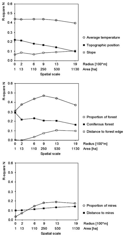
We defined the best scale for every independent variable by comparing their explained variance (R2N) in univariate logistic regression models at all
six spatial scales analyzed (Figure 2). Some vari-ables performed best at small scales (e.g. topo-graphic position, coniferous forest), others at large scales (e.g. proportion of forest). Other variables were not sensitive towards the observed spatial scale (e.g. average temperature). Variables that had the highest predictive power in univariate models were ‘proportion of forest’, ‘average tem-perature’ and ‘coniferous forest’ (R2N= 0.44,
Multivariate models
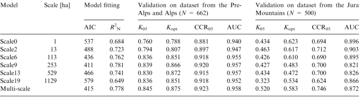
To calibrate the multivariate models, we retained eight independent variables that were not highly inter-correlated and had a minimum R2Nof 0.05 in
the univariate models. We also included the squared term of four variables to account for unimodal responses to capercaillie presence– absence. Generally, all multivariate models (single-scale and multi-(single-scale) performed well on data from the calibration area that were set aside for vali-dation (0.76 < K05< 0.85; 0.94 < AUC < 0.96;
Table 2).
Within the group of the single-scale models, where all variables were included at the same
spatial scale, we found predictive power to be highest at the intermediate scales (113 and 253 ha; Table 2), with the model at a scale of 253 ha (radius 900 m) performing best (R2N= 0.781,
K05= 0.839, AUC = 0.957). The multi-scale
model that included every variable at its best scale attained a similar accuracy (R2N= 0.778,
K05= 0.845, AUC = 0.958) as the best
single-scale model (Figure 3). In the validation on the independent dataset from the Jura Mountains, the multi-scale model classified best when the same threshold value (0.5) was used as in the model calibration (K05 = 0.520; compared to 0.323 <
K05< 0.436 of the single-scale models). At the
optimized threshold value, the two single-scale
Table 2. Accuracy of single-scale models (scale0–scale19) and the multi-scale model; accuracy measures for model fitting (AIC, R2 N)
and validation (K05, Kopt, CCR05, AUC).
Model Scale [ha] Model fitting Validation on dataset from the Pre-Alps and Pre-Alps (N = 662)
Validation on dataset from the Jura Mountains (N = 500)
AIC R2
N K05 Kopt CCR05 AUC K05 Kopt CCR05 AUC
Scale0 1 537 0.684 0.760 0.788 0.881 0.940 0.434 0.623 0.694 0.896 Scale2 13 488 0.723 0.794 0.807 0.897 0.947 0.463 0.617 0.712 0.903 Scale6 113 436 0.762 0.836 0.851 0.918 0.955 0.426 0.610 0.690 0.895 Scale9 253 411 0.781 0.839 0.866 0.920 0.957 0.427 0.483 0.700 0.821 Scale13 529 466 0.741 0.830 0.872 0.915 0.957 0.434 0.472 0.700 0.826 Scale19 1129 579 0.649 0.836 0.851 0.918 0.952 0.323 0.534 0.624 0.866 Multi-scale 415 0.778 0.845 0.875 0.923 0.958 0.520 0.583 0.746 0.872
Figure 3. Accuracy of single-scale and multi-scale models calibrated on the combined dataset of the Alps and Pre-Alps; model fitting (R-square Nagelkerke) and validation using set-aside data from the Pre-Alps and Alps (Kappa_05) and from the Jura Mountains (Kappa_05_Jura).
models working at the smallest spatial scales performed best (Kopt= 0.623, and 0.617,
respec-tively).
The same variable set had been used for the calibration of the multi-scale and single-scale models. From this set, all single-scale and multi-scale models retained almost the same combina-tion of variables. Those variables were ‘average temperature’, ‘proportion of forest’, ‘topographic position’, ‘slope’ and ‘proportion of mires and wet forest’ (Table 3). Most models retained the squared terms of ‘average temperature’ and ‘slope’, indicating a unimodal response to caper-caillie presence–absence. In the multi-scale model, ‘coniferous forest’ was retained as an additional variable.
The models not only differ in their accuracy, but also in the proportion and distribution of predicted presence area when applied on the study area
(Figure 4). The mean proportion of predicted presence area of the single-scale models ranges from 18.0% (scale0) to 23.5% (scale19). The mean patch size increases from 38.4 ha (scale0) to 2050.1 ha (scale19). The multi-scale model, in which we in-cluded all variables at the best-explaining scale, shows intermediate values (proportion of presence area: 19.6%, mean patch size: 240.9 ha).
Sensitivity test of presence/absence definition One could argue that our models have high accuracy values because we included a buffer zone of 1000 m between presence and absence cells, and thus many grid cells with intermediate suitability were excluded from the validation. To test the degree to which the buffer size influences model accuracy, we decreased buffer size stepwise (1000,
Table 3. Variables included in the single-scale and multi-scale models; p-values of logistic regression; best scale: scale at which a variable was entered in the multi-scale model.
Variable Best scale [ha] Scale0 1 ha Scale2 13 ha Scale6 113 ha Scale9 253 ha Scale13 529 ha Scale19 1129 ha Multi-scale Proportion of forest 253 <0.001 <0.001 <0.001 <0.001 <0.001 <0.001 <0.001 Average temperature 1 <0.001 <0.001 <0.001 <0.001 <0.001 <0.001 <0.001 Average temperature2 1 <0.001 <0.001 <0.001 <0.001 <0.001 <0.001 <0.001 Topographic position 1 <0.001 <0.001 <0.001 <0.001 <0.001 <0.001 <0.001 Slope 13 0.002 0.012 Slope2 13 <0.001 <0.001 <0.001 <0.001 0.001 <0.001 <0.001 Proportion of mires 529 0.004 <0.001 0.001 <0.001 <0.001 0.002 <0.001 Coniferous forest 1 0.033
Figure 4. Distribution of predicted presence areas for different models (a–d) and observed presence (e); (a) scale0: window size 1 ha, (b) scale9: window size 253 ha, (c) scale19: window size 1129 ha, (d) multi-scale model, (e) observed presence.
750, and 500 m) and thereby allowed more absence cells near capercaillie presence in the validation dataset. The accuracy of the multi-scale model decreased with decreasing buffer size, yet remained on a high level: buffer of 1000 m (K05= 0.845,
AUC = 0.958), 750 m (K05= 0.777, AUC =
0.940), 500 m (K05= 0.727, AUC = 0.934).
Decreasing model accuracy resulted from the decreasing positive predictive power (0.892, 0.813, 0.761), which means that there will be more grid cells that are wrongly classified as ‘presence’. An analogous decrease of model accuracy and positive predictive power was found for the single-scale models (data not shown).
Spatial autocorrelation of residuals
Only weak spatial autocorrelation was found in the residuals of the multivariate models at the two largest scales. Moran’s I was significantly different from zero in the residuals of the models at 529 ha (Moran’s I=0.048, p<0.050) and 1129 ha (Moran’s I=0.081, p<0.001). The residuals of the multi-scale model showed no significant spatial correlation (Moran’s I=0.012, p=0.202). Given the weak spatial dependence of the residuals at the level of the first neighbor, we did not perceive a need to calculate correlograms and to further investigate spatial autocorrelation.
Discussion
The present study confirms other findings that species respond to ecological parameters at par-ticular spatial scales. Based on our results, we will consider three main issues: First, we discuss the significance of scale for capercaillie occurrence in mountain landscapes and compare the single-scale with the multi-scale approach. Second, we address the high prediction success of the multivariate models. Third, we discuss the implications of the habitat parameters identified by the models as being important at the landscape scale.
Spatial scale
Spatial scale matters when habitat selection by capercaillie is studied. By comparing a number of
single-scale models, we found the best grain size to be about 250 ha for habitat models for capercaillie. The value of 250 ha is equivalent to the size of a small annual home range (Rolstad et al. 1988; Storch 1995). Most studies of home range size use minimum convex polygons, i.e. a method that tends to overestimate the area actually used by the birds. Thus, our results support the suggestion that habitat selection of space-demanding large verte-brates may be dominated by factors operating at the home-range scale and above (Carroll et al. 1999).
Optimizing the spatial scale for each variable and calculating an optimized, multi-scale model proved to be a promising approach. Some vari-ables explained species occurrence better at small scales, while others did better at large scales. This is in agreement with our hypothesis that the capercaillie responds to its environment at differ-ent spatial scales at the same time. Similar scale dependence of single habitat variables was found for reptiles (Fischer et al. 2004) or the bald eagle (Haliaeetus leucocephalus), another space-demanding bird species (Thompson and McGarigal 2002). In our case, the multi-scale model per-formed equally well as the best single-scale models when tested on independent data from the cali-bration area. However, the multi-scale model proved to be superior in the test on independent data from another, different area. Thus, the multi-scale approach seems to capture the species-habitat relationship in a more mechanistic way that leads to greater model generality. Consequently, we recommend that variables in multivariate habitat distribution models should be included at different spatial scales.
The models at the various spatial scales differ in accuracy, but all models reach good accuracy values (Kappa > 0.7). However, the resolution of predicted presence areas (Figure 4) depends on the spatial scale of the model. According to the objectives of a particular analysis, we might find different spatial scales to be the most appropriate ones. For instance, when aiming at identifying potentially suitable forest patches, we will proba-bly use a model developed at a relatively small scale. For studying the distribution and connec-tivity of populations or providing a basis for meta-population modeling, a large-scale model would possibly be more appropriate. Additionally, model accuracy strongly depends on the scale and
coding of the response variable (Cushman and McGarigal 2004). In our study, however, the scale of the presence–absence data was kept constant.
Predictive ability of the models
Model predictions were quite good. We attribute this to two reasons: First, habitat preferences of capercaillie are specialized also at the landscape scale, so that a few of the common landscape-scale variables are capable of predicting capercaillie occurrence to a large extent. Second, our definition of presence and absence is probably bound to produce (relatively) good model predictions and must be considered in detail. In order to avoid false observed absences in the calibration and validation dataset, we applied a buffer of one kilometer around the presence points. This buffer led to ‘tolerant’ habitat models that predict a high probability of capercaillie presence for almost all areas with capercaillie observations. Because we included a buffer around the observed presence cells, most observed absence cells were also clas-sified correctly. By reducing the buffer in the val-idation process, the rate of false positives is increasing while the number of false negatives is remaining low. Still, the overall model accuracy remains high. Thus, we conclude that our approach is quite robust.
Variables selected by the models
Our results confirm that a small set of landscape-scale variables can explain capercaillie presence–absence to a considerable extent. They also support the conclusion of Storch (2002) that factors operating at the landscape scale could ex-plain the variance of capercaillie occurrence that was not explained by small-scale habitat prefer-ences.
Only few variables explain capercaillie occur-rence in our models: proportion of forest, average temperature, topography, slope and proportion of mires and wet forests. Capercaillie preferably occur in large and well-connected forest tracts (Storch 1995; Kurki et al. 2000). This general finding is confirmed by the high significance of the variable ‘proportion of forest’ in our models and concretized by the best scale of a small home range
(250 ha) that we could detect for this variable. As expected, average temperature accounted for much of the explained variance in the multivariate models, since capercaillie in Switzerland (and most other parts of Central Europe) is restricted to a range of altitude starting at 800 m and extending to the upper tree line at 1600–2200 m a.s.l. This altitudinal range in Central Europe offers similar climate and similar coniferous forest vegetation as the boreal climate zone where optimal habitats for capercaillie are spread over large areas. Influence of topography on capercaillie habitat use has al-ready been found in Central European popula-tions (Storch 2002; Suchant 2002). Our results confirm that capercaillie prefer gentle slopes to precipitous topography. Additionally, capercaillie records are made more often on mountain ridges or upper slopes than in toe slopes or valley bottoms.
Some variables did not enter in our multivariate models but may nevertheless have an influence on capercaillie distribution. Some variables (e.g. road density, distance to settlements) are highly sig-nificant in the univariate models (R2N= 0.184, 0.129, respectively), but they do not enter in the multivariate models. This is due to our strict cri-teria of including or excluding a variable in the multivariate models, which we applied in order to keep the models simple for the comparison between the different spatial scales. We allowed only a low level of collinearity (Spearman’s q < 0.5) between two variables. Additionally, we used a significance level of 0.05 for retaining a variable in a model, whereas other authors have argued for a threshold of 0.1 (Schro¨der 2000) or even 0.2 (Hosmer and Lemeshow 1989; Menard 2002). Thus, we possibly excluded some variables from the analysis that, in reality, have an influ-ence on capercaillie occurrinflu-ence.
Our habitat models do not contain any infor-mation on small-scale habitat quality such as forest structure, cover of field layer, or cover of bilberry Vaccinium myrtillus. They can thus be regarded as simulating potential capercaillie hab-itat. This is supported by the fact that most predicted-presence areas without actual caper-caillie records have indeed had capercaper-caillie a few decades ago (Mollet et al. 2003). Therefore, areas with predicted presence may have been aban-doned by capercaillie because of reasons operat-ing at smaller spatial scales. For instance, forest
structure may have become unsuitable or the areas may be disturbed frequently because of human activities (recreation, hunting, etc.). These considerations are relevant when we apply our models in practice: areas with suitable landscape structure (predicted presence) but presently with-out capercaillie could possibly be populated again if forest structure was improved and human dis-turbance was reduced.
Conclusions
Our multivariate models at the landscape scale predict capercaillie occurrence to a large extent and add significant insights in capercaillie habitat relationships at larger scales. The multi-scale ap-proach is promising because it led to precise and at the same time general models and produced plau-sible distribution maps with an intermediate degree of detail. These maps can be used directly for large-scale conservation planning and as a basis for spatially explicit meta-population modeling.
Nevertheless, more detailed analyses of predic-tor variables are necessary to better understand the processes in habitat selection of capercaillie at large spatial scales. Do species-habitat relation-ships vary between different regions and to what extent? How does the coding of the response var-iable (presence–absence of capercaillie) influence the model prediction? Such questions should be addressed by comparing our ‘general’ models with regional models calibrated in sub-regions of the study area.
In spite of the classification success of our large-scale models, considerable attention has to be paid to small-scale habitat quality. For instance, we need to know more about the requirements of capercaillie regarding the amount and spatial arrangement of suitable habitats. Combining our large-scale approach with data describing habitat quality at the scale of forest stands would allow us to develop effective tools for capercaillie conservation.
Acknowledgements
We thank Niklaus E. Zimmermann, Curtis H. Flather and two anonymous reviewers for comments on the manuscript. Financial support
for this publication was provided by the Swiss National Science Foundation (SNF) and the Swiss Federal Agency for the Environment, Forest and Landscape (BUWAL). The Swiss Ornithological Institute, the ‘Centre de conservation de la faune et de la nature’ of the canton of Vaud and several local grouse experts provided large datasets on capercaillie occurrence.
References
Augustin N.H., Mugglestone M.A. and Buckland S.T. 1996. An autologistic model for the spatial distribution of wildlife. J. Appl. Ecol. 33: 339–347.
Baines D., Moss R. and Dugan D. 2004. Capercaillie breeding success in relation to forest habitat and predator abundance. J. Appl. Ecol. 41: 59–71.
Berg A., Ga¨rdenfors U. and von Proschwitz T. 2004. Logistic regression models for predicting occurrence of terrestrial molluscs in Sweden – importance of environmental data quality and model complexity. Ecography 27: 83–93. Bissonette J.A. 1997. Scale-sensitive ecological properties:
his-torical context, current meaning. In: Bissonette J.A. (ed.), Wildlife and Landscape Ecology: Effects of Pattern and Scale. Springer-Verlag, New York, pp. 3–31.
Boyce M.S., Vernier P.R., Nielsen S.E. and Schmiegelow F.K.A. 2002. Evaluating resource selection functions. Ecol. Model. 157: 281–300.
Carroll C., Zielinski W.J. and Noss R.F. 1999. Using presence– absence data to build and test spatial habitat models for the fisher in the Klamath region, USA. Conserv. Biol. 13: 1344–1359.
Cushman S.A. and McGarigal K. 2004. Patterns in the species-environment relationship depend on both scale and choice of response variables. Oikos 105: 117–124.
Deleo J.M. 1993. Receiver operating characteristic laboratory (ROCLAB): software for developing decision strategies that account for uncertainty. In: First International Symposium on Uncertainty Modelling and Analysis. IEEE, Computer Society Press, College Park, MD.
Elkie P.C., Rempel R.S. and Carr A.P. 1999. Patch Analyst User’s Manual: A Tool for Quantifying Landscape Structure. Ontario Ministry of Natural Resources, Northwest Science and Technology, Thunder Bay, Ontario, Canada.
Fielding A.H. and Bell J.F. 1997. A review of methods for the assessment of prediction errors in conservation presence/ absence models. Environ. Conserv. 24: 38–49.
Fielding A.H. and Haworth P.F. 1995. Testing the generality of bird-habitat models. Conserv. Biol. 9: 1466–1481.
Fischer J., Lindenmayer D.B. and Cowling A. 2004. The challenge of managing multiple species at multiple scales: reptiles in an Australian grazing landscape. J. Appl. Ecol. 41: 32–44.
Freemark K.E. and Merriam H.G. 1986. Importance of area and habitat heterogeneity to bird assemblages in temperate forest fragments. Biol. Conserv. 36: 115–141.
Fuhlendorf S.D., Woodward A.J.W., Leslie D.M.Jr. and Shackford J.S. 2002. Multi-scale effects of habitat loss and
fragmentation on lesser prairie-chicken populations of the US Southern Great Plains. Landscape Ecol. 17: 617–628. Gibson D.J., Wilson B.A., Cahill D.M. and Hill J. 2004. Spatial
prediction of rufous bristlebird habitat in a coastal heath-land: a GIS-based approach. J. Appl. Ecol. 41: 213–223. Guisan A. and Zimmermann N.E. 2000. Predictive habitat
distribution models in ecology. Ecol. Model. 135: 147–186. Hosmer D.W. and Lemeshow S. 1989. Applied Logistic
Regression. John Wiley & Sons, New York.
Johnson C.J., Seip D.R. and Boyce M.S. 2004. A quantitative approach to conservation planning: using resource selection functions to map the distribution of mountain caribou at multiple spatial scales. J. Appl. Ecol. 41: 238–251.
Keppie D.M. and Kierstead J.M. 2003. The need to improve our attention to scale of resolution in grouse research. Wildlife Biol. 9: 385–391.
Klaus S., Andreev A.V., Bergmann H.-H., Mu¨ller F., Porkert J. and Wiesner J. 1986. Die Auerhu¨hner. A. Ziemsen Verlag, Wittenberg Lutherstadt, Germany.
Klaus S., Boock W., Go¨rner M. and Seibt E. 1985. Zur O¨kologie des Auerhuhns (Tetrao urogallus L.) in Thu¨ringen. Acta Ornithoecol. 1: 3–46.
Kumar L., Skidmore A.K. and Knowles E. 1997. Modelling topographic variation in solar radiation in a GIS environ-ment. J. Geogr. Inf. Syst. 11: 475–497.
Kurki S. and Linden H. 1995. Forest fragmentation due to agri-culture affects the reproductive success of the ground-nesting black grouse Tetrao tetrix. Ecography 18: 109–113.
Kurki S., Nikula A., Helle P. and Linden H. 2000. Landscape fragmentation and forest composition effects on grouse breeding success in boreal forests. Ecology 81: 1985–1997. Lawler J.J. and Edwards T.C. Jr. 2002. Landscape patterns
as habitat predictors: building and testing models for cavity-nesting birds in the Uinta Mountains of Utah, USA. Landscape Ecol. 17: 233–245.
Levin S.A. 1992. The problem of pattern and scale in ecology. Ecology 73: 1943–1967.
Mace R.D., Waller J.S., Manley T.L., Ake K. and Wittinger W.T. 1999. Landscape evaluation of grizzly bear habitat in western Montana. Conserv. Biol. 13: 367–377.
MacFaden S.W. and Capen D.E. 2002. Avian habitat rela-tionships at multiple scales in a New England forest. For. Sci. 48: 243–253.
Manly B.F.J., McDonald L.L., Thomas D.L., McDonald T.L. and Erickson W.P. 2002. Resource Selection by Animals – Statistical Design and Analysis for Field Studies. Kluwer Academic Publishers, Dordrecht, Netherlands.
McGarigal K., Cushman S.A. and Neel M.C. 2002. FRAG-STATS: Spatial Pattern Analysis Program for Categorical Maps. Computer Software Program produced by the authors at the University of Massachusetts, Amherst, USA. Menard S. 2002. Applied Logistic Regression Analysis. Sage
Publications, London.
Mladenoff D.J. and Sickley T.A. 1998. Assessing potential gray wolf restoration in the northeastern United States: a spatial prediction of favorable habitat and potential population levels. J. Wildlife Manage. 62: 1–10.
Mollet P., Badilatti B., Bollmann K., Graf R.F., Hess R., Jenny H., Mulhauser B., Perrenoud A., Rudmann F., Sachot S. and Studer J. 2003. Verbreitung und Bestand des Auerhuhns Tetrao urogallusin der Schweiz 2001 und ihre Vera¨nderungen
im 19. und 20. Jahrhundert. Der Ornithologische Beobachter 100: 67–86.
Monserud R.A. and Leemans R. 1992. Comparing global vegetation maps with the Kappa statistics. Ecol. Model. 62: 275–293.
Moran P.A.P. 1948. The interpretation of statistical maps. J. R. Stat. Soc. 10: 243–251.
Moss R., Oswald J. and Baines D. 2001. Climate change and breeding success: decline of the capercaillie in Scotland. J. Anim. Ecol. 70: 47–61.
Nagelkerke N.J.D. 1991. A note on a general definition of the coefficient of determination. Biometrika 78: 691–692. Pearce J. and Ferrier S. 2000. An evaluation of alternative
algorithms for fitting species distribution models using lo-gistic regression. Ecol. Model. 128: 127–147.
Rolstad J. and Wegge P. 1989. Capercaillie populations and modern forestry – a case for landscape ecological studies. Finnish Game Res. 46: 43–52.
Rolstad J., Wegge P. and Larsen B.B. 1988. Spacing and habitat use of capercaillie during summer. Can. J. Zool. 66: 670–679. Roth P. and Nievergelt B. 1975. Die Standorte der Balzpla¨tze beim Auerhuhn (Tetrao urogallus). Der Ornithologische Be-obachter 72: 101–112.
Rushton S.P., Ormerod S.J. and Kerby G. 2004. New para-digms for modelling species distributions? J. Appl. Ecol. 41: 193–200.
Sachot S., Perrin N. and Neet C. 2003. Winter habitat selection by two sympatric forest grouse in western Switzerland: implications for conservation. Biol. Conserv. 112: 373–382. Schro¨der B. 2000. Zwischen Naturschutz und Theoretischer
O¨kologie: Modelle zur Habitateignung und ra¨umlichen Pop-ulationsdynamik fu¨r Heuschrecken im Niedermoor. Ph.D. Thesis, Technische Universita¨t Braunschweig, Braunschweig, Germany, 228 pp.
Schro¨der B. 2002. Habitatmodelle fu¨r ein modernes Naturs-chutzmanagement. In: Gnauck A. (ed.), Workshop Ko¨lpinsee 2000. Shaker, Aachen, Germany, pp. 201–224.
Schroth K.-E. 1992. Zum Lebensraum des Auerhuhns (Tetrao urogallus L.) im Nordschwarzwald. Ph.D. Thesis, Universita¨t Mu¨nchen, Mu¨nchen, Germany, 129 pp.
Segelbacher G., Storch I. and Tomiuk J. 2003. Genetic evidence of capercaillie Tetrao urogallus dispersal sources and sinks in the Alps. Wildlife Biol. 9: 267–273.
Sjo¨berg K. 1996. Modern forestry and the capercaillie. In: DeGraaf M. and Miller R.I. (eds), Forested Landscapes. Chapman & Hall, London, pp. 111–135.
Smith P.A. 1994. Autocorrelation in logistic regression model-ling of species’ distributions. Global Ecol. Biogeogr. Lett. 4: 47–61.
Steiger P. 1994. Wa¨lder der Schweiz. Ott Verlag, Thun, Switzerland.
Storch I. 1994. Habitat and survival of capercaillie Tetrao urogallusnests and broods in the bavarian alps. Biol. Con-serv. 70: 237–243.
Storch I. 1995. Annual home ranges and spacing patterns of capercaillie in Central Europe. J. Wildlife Manage. 59: 392–400. Storch I. 1997. The importance of scale in habitat conservation for an endangered species: the capercaillie in Central Europe. In: Bissonette J.A. (ed.), Wildlife and Landscape Ecology: Effects of Pattern and Scale. Springer-Verlag, New York, pp. 310–330.
Storch I. 2000a. Conservation status and threats to grouse worldwide: an overview. Wildlife Biol. 6: 195–204.
Storch I. (ed.), 2000b. Grouse status survey and Conservation Action Plan 2000–2004 WPA/BirdLife/SSC Grouse Specialist Group. IUCN, Gland, Switzerland and Cambridge, UK and the World Pheasant Association, Reading, UK.
Storch I. 2002. On spatial resolution in habitat models: can small-scale forest structure explain capercaillie numbers? Conserv. Ecol. 6(1): 6 [online] URL: http://www.consecol. org/vol6/iss1/art6.
Storch I. and Segelbacher G. 2000. Genetic correlates of spatial population structure in central European capercaillie Tetrao urogallusand black grouse T-tetrix: a project in progress. Wildlife Biol. 6: 305–310.
Suchant R. 2002. Die Entwicklung eines mehrdimensionalen Habitatmodells fu¨r Auerhuhnareale (Tetrao urogallus L.) als Grundlage fu¨r die Integration von Diversita¨t in die Waldbaupraxis. Ph.D. Thesis, Universita¨t Freiburg, Frei-burg, Germany, 331 pp.
Thompson C.M. and McGarigal K. 2002. The influence of research scale on bald eagle habitat selection along the lower
Hudson River, New York (USA). Landscape Ecol. 17: 569–586.
Wegge P. and Larsen B.B. 1987. Spacing of adult and subadult male common capercaillie during the breeding season. Auk 104: 481–490.
Wegge P. and Rolstad J. 1986. Size and spacing of capercaillie leks in relation to social behaviour and habitat. Behav. Ecol. Sociobiol. 19: 401–408.
Wiens J.A. 1989. Spatial scaling in ecology. Funct. Ecol. 3: 385–397.
Zabel C.J., Dunk J.R., Stauffer H.B., Roberts L.M., Mulder B.S. and Wright A. 2003. Northern spotted owl habitat models for research and management application in Cali-fornia (USA). Ecol. Appl. 13: 1027–1040.
Zimmermann N.E. and Kienast F. 1999. Predictive mapping of alpine grasslands in Switzerland: species versus community approach. J. Veg. Sci. 10: 469–482.
Zimmermann N.E. and Roberts D.W. 2001. Final report of the MLP climate and biophysical mapping project. Swiss Federal Research Institute WSL/Utah State University, Birmensdorf, Switzerland/Logan, USA, 18 pp.