Depth and homogeneity in regional flood frequency analysis

Depth and homogeneity in regional flood frequency analysis

1

2

F. Chebana

*

and T.B.M.J. Ouarda

3

4 5

Industrial Chair in Statistical Hydrology/Canada Research Chair on the Estimation of

6

Hydrometeorological Variables,

7

INRS-ETE, 490 rue de la Couronne, Quebec (QC),

8 Canada G1K 9A9 9 10 11 12 13 14 15 16 *

Corresponding author: Tel: (418) 654-2542

17 Fax: (418) 654-2600 18 Email: fateh_chebana@ete.inrs.ca 19

July 11

th

2008

20 21 22 23 24

Abstract:

1

Regional frequency analysis (RFA) consists generally in two steps: 1) delineation of 2

hydrological homogeneous regions, and 2) regional estimation. Existing regionalization methods 3

which adopt this two-step approach suffer from two principal drawbacks. First, the restriction of 4

the regional estimation to a particular region by excluding some sites can correspond to a loss of 5

some information. Second, the definition of a region generates a border effect problem. In order 6

to overcome these problems, a new method is proposed in the present paper. The proposed 7

method is based on three elements: (i) a weight function to treat the border effect problem, (ii) a 8

function to evaluate how “similar” each site is to the target one, and (iii) an iterative procedure to 9

improve estimation results. Element (ii) is treated using the statistical notion of depth functions 10

which is introduced to provide a ranking of stations in a multivariate context. Furthermore, the 11

properties of depth functions meet the characteristics sought in RFA. It is shown that the 12

proposed method is flexible and general and that traditional RFA methods represent special cases 13

of the depth-based approach corresponding to particular weight functions. A comparison is 14

carried out with the canonical correlation analysis (CCA) approach. Results indicate that the 15

depth-based approach performs better than CCA both in terms of relative bias and relative root 16

mean squares error. 17

1. Introduction

1

One of the problems encountered in hydrology is the lack of data, since the extreme 2

events we want to estimate are rare and record lengths are short. Consequently, statistical 3

inference is difficult in such sites. To overcome this problem, hydrologists have recourse to data 4

from other sites that are hydrologically similar to the target one. The estimation of extreme 5

hydrological events, such as floods, at sites where little or no data is available is the main aim of 6

regional frequency analysis. Delineation of homogeneous hydrological regions and regional 7

estimation are the two main steps in a regional flood frequency procedure. Several studies have 8

focused on the delineation of homogeneous regions (e.g., Burn, 1990; Hosking and Wallis, 1993; 9

Ouarda et al., 2006; and Chebana and Ouarda, 2007) and on regional estimation (e.g., Dalrymple, 10

1960; Stedinger and Tasker, 1986; Ouarda and Ashkar, 1994; Durrans and Tomic, 1996; Nguyen 11

and Pandey, 1996; Madsen and Rosbjerg, 1997; Alila, 1999, 2000 and Chokmani and Ouarda, 12

2004). An intercomparison of various regional flood estimation procedures was presented by 13

GREHYS (1996a,b) by coupling four methods for delineating homogenous regions and seven 14

regional estimation methods. 15

16

In a regional estimation procedure, one is interested in maximizing the amount of 17

transferred information. The delineation step corresponds usually to the exclusion of a number of 18

sites which may lead to a loss of some relevant information. Furthermore, the definition of a 19

region leads to the problem of the so-called “border effect”. This means that for two sites that are 20

very close but which are located on each side of the region limits, one is excluded while the other 21

one is included even though both sites offer similar information. This problem is not present 22

when the limits correspond to natural borders. 23

These elements motivate the development of a new method that overcomes some of these 1

drawbacks. The method developed in the present paper is based on the notion of depth function. 2

The depth function is a statistical notion developed in the seventies and which receives increasing 3

interest (e.g. Tukey, 1975; Liu, 1990; Liu and Singh, 1993; Rousseeuw and Hubert, 1999; Zuo 4

and Serfling, 2000; Mizera, 2002; Mizera and Müller. 2004; Zuo and Cui, 2005 and Lin and 5

Chen, 2006). The purpose for introducing the depth function is to provide an outward ordering of 6

points in a multivariate context. The most important properties of a depth function are (i) affine 7

invariance, (ii) maximality at center, (iii) monotonicity related to the deepest point, and (iv) 8

vanishing at infinity. These properties fit the constraints of regional flood frequency analysis. 9

Indeed, the affine invariance is useful to remove the scale effect when treating several variables. 10

The center, where the depth function is maximal, represents the target site. The monotonicity 11

related to the center point means that sites far from the target site are less important. Finally, the 12

very far sites have no importance or no contribution; this is the vanishing at infinity property. 13

Hence, the contribution of each site is related to its similarity to the target site. 14

15

The proposed procedure focuses on the estimation as a goal and avoids the delineation 16

step. Note that the delineation step is only an intermediate technical tool to estimate quantiles. 17

Different quantile estimation methods are proposed in the literature, such as the index flood 18

method and regressive models (see GREHYS, 1996a,b). In the present paper, the estimation is 19

based on the regressive model. The estimation of the regression parameters is obtained using a 20

weighted least squares method. A key element is related to the choice of the weights. These 21

weights are selected as functions of the site depth. Hence, the proposed method overcomes the 22

Furthermore, traditional approaches represent special cases of depth-based approaches 1

corresponding to particular weight functions. Finally, the non requirement of data normality, the 2

availability of several kinds of depth functions and the smoothness of the weight functions 3

provide this method with a high level of flexibility. 4

5

Based on hydrological variables, on one hand, and on physio-meteorological 6

characteristics, on the other hand, regional regression is frequently integrated with the CCA 7

approach (Ouarda et al., 2000, 2001). The CCA-regression provides flood quantile estimates at 8

ungauged sites by using site physiographic characteristics. In order to study the performance of 9

the proposed depth-based approach, it is compared to the CCA-regression approach with optimal 10

neighborhoods (Ouarda et al., 2001). This comparison is based on a data set from 151 gauging 11

sites in the southern part of the province of Quebec, Canada. The specific quantiles 12

corresponding to 10- and 100-year return periods are estimated and a jackknife resampling 13

procedure is used to evaluate the estimation errors. 14

15

The paper is organized as follows. Brief presentations of the depth functions, the CCA 16

approach and the weighted least squares method are given in Section 2. Section 3 deals with the 17

proposed methodology in its general form. A case study is presented in Section 4 and the 18

developed approach is applied and compared to the CCA method in Section 5. Results and 19

discussions are reported in Section 6. Conclusions and future promising work are presented in the 20

last section. 21

22 23

2. Background

1

In this section, a brief description of the background material related to depth functions, 2

the CCA method and weighted regression analysis is presented. 3

4

2.1 Depth function:

5

Tukey (1975) presented the pioneering work in which the depth notion was introduced. 6

The author proposed a halfspace depth in order to define a multivariate analogous to the 7

univariate rank and order statistics. Later, several depth functions were formulated in an ad-hoc 8

manner. Zuo and Serfling (2000) standardized these definitions and classified existing examples 9

in the literature. 10

11

For a given cumulative distribution function F on d ( 1)

R d ≥ a corresponding depth 12

function is any bounded, nonnegative function D(x;F) which provides a F-based center-outward 13

ordering of points x in _{ℝ that satisfies the following properties:} d 14

i. Affine invariance: the depth of a point x∈Rd should not depend on the underlying 15

coordinate system or, in particular, on the scales of the underlying measurements. 16

ii. Maximality at center: for a distribution having a uniquely defined center (e.g., the point of 17

symmetry with respect to some notion of symmetry), the depth function should attain its 18

maximum value at this center. 19

iii. Monotonicity relative to deepest point: as a point x∈Rd moves away from the deepest 20

point (the point at which the depth function attains its maximum value; in particular, for a 21

symmetric distribution, the center) along any fixed ray through the center, the depth at x 22

iv. Vanishing at infinity: the depth of a point x should approach zero as its norm x

1

approaches infinity. 2

3

A formal definition of depth functions, based on these properties, is given in Zuo and 4

Serfling (2000). In the following, we denote by ∆ the class of cumulative distribution functions 5

on Rd and by F_Z the cumulative distribution function of a given random vector Z. Let the 6

mapping D(.;.) :Rd× ∆ → be bounded, non-negative, and satisfy the following conditions: R

7

i. D Ax( +b F; _{AX b+} )=D x F( ; _X) holds for any random vector X in Rd , any 8

d× nonsingular matrix A, and any d-vector b; d

9

ii. D( ; )θ F =sup_{x R∈} d D x F( ; ) holds for any F ∈ ∆ having center θ ; 10

iii. For any F ∈ ∆ having deepest point θ , D x F( ; )≤D

(

θ α

+ (x−

θ

) ;x F

)

holds for 11

[

0, 1

]

α

∈ ; and 12

iv. D x F( ; ) converges to 0 as the norm x goes to infinity, for each F∈ ∆ . 13

Then D(.; )F is called a statistical depth function. 14

15

Several kinds of depth functions are introduced in the literature. Here we present some of 16

the key ones: 17

1. Mahalanobis depth: It is defined on the basis of the Mahalanobis distance 18

(

) (

)

(

)

2 1

, A

d x y = x−y ′A− x− y between two points , d

x y∈R with respect to a positive 19

definite matrix A (Mahalanobis, 1936). The Mahalanobis depth is then given by: 20

(

)

2 1 ( ; ) 1 _A , MHD x F d x

µ

= + (1) 21

where F is a given distribution and µ and A are any corresponding location and 1

covariance measures, respectively. Note that the Mahalanobis distance is used in the 2

development of the CCA approach for regional flood frequency analysis (Ouarda et al., 3

2001). It is also important to note that the Mahalanobis depth function has values in the 4

interval

[ ]

0,1 . Hence, its values are more interpretable than those of the corresponding 5

Mahalanobis distance. 6

2. L2 depth: It is defined for a distribution F and x∈Rd as: 7 1 2 1 ( ; ) 1 L D x F E x X _Σ− = + − (2) 8

where Σ is the covariance matrix of F and x _M = x Mx′ . 9

3. Simplicial volume depth (Oja, 1983): It is given through the expression : 10

[

]

(

)

( )

1 1 , ,..., ( , ) 1 for det d d S x X X SVD x F E x R α α −  _{∆ }   _{ }  =_ + _ ∈  _Σ    _{  }   (3) 11

where ∆

(

S x X

[

, 1,...,Xd

]

)

denotes the volume of the d-dimensional simplex 12

[

, 1,..., d

]

S x X X , Σ is the covariance matrix of F and α >0. The quantity 13

[

]

(

S x X, 1,...,Xd

)

∆ is a measure of the dispersion of the point cloud. 14

4. Projection depth (Liu, 1992): It is defined for x∈Rd as : 15

(

)

₍

(

₎

)

1 1 Med ; 1 sup MAD u u x u X PD x F u X − =  ′ − ′  =_ + _′ _   (4) 16

where X has distribution F, Med denotes the univariate median, 1

(

)

MAD( )Y =Med Y −Med( )Y represents the median absolute deviation for a random 2

variable Y, and ⋅ is the Euclidian norm. 3

5. Halfspace depth (Tukey, 1975): It is defined for x∈Rdwith respect to a probability P on 4

d

R as:

5

(

;

)

inf

{

( ) : a closed halfspace that contains

}

HD x P = P H H x (5)

6 7

Note that, occasionally, some examples of depth functions do not meet some of the 8

previous four properties in some special cases. For instance, the 2

( ; )

L D x F function only meets

9

the above conditions under symmetric assumptions on the distribution F (see Zuo and Serfling, 10

2000). 11

12

A sample version of D(x;F), denoted by D x_n( )=D x F( ; ˆ_n), may be defined by replacing F 13

with a suitable empirical function Fˆ_n. The asymptotic properties of D x are studied in several _n( ) 14

papers including Liu (1990), Arcones et al. (1994), Massé (2004) and Lin and Chen (2006). Liu 15

and Singh (1993) established for the sample Mahalanobis depth function that 16

sup _n( ) ( ; ) x

D x −D x F converges to zero almost surely as n goes to infinity, under suitable 17

conditions on F. For convenience, the following notation is used for the Mahalanobis depth 18

function in the next sections: 19

(

)

2 1 ( ; ) 1 , A A MHD x d x

µ

µ

= + (6) 20

Depth functions are applied in several fields. For instance, Caplin and Nalebuff (1988, 1

1991a,b) employed depth notions in econometric and social studies. They were also applied in 2

industrial quality control by Liu and Singh (1993) and Liu (1995). Ghosh and Chaudhuri (2005) 3

investigated the use of depth functions in nonparametric discrimination analysis. Mizera and 4

Müller (2004) defined and studied the location-scale depth and gave some statistical applications. 5

6

The computation of some depth functions is complex and requires specific algorithms. 7

For instance, Miller et al. (2003) developed an algorithm for the computation of the halfspace 8

depth. However, to our knowledge, similar algorithms are not available for the projection depth. 9

The Mahalanobis depth is among the simplest ones to evaluate if the parameter µ and the 10

parameter matrix A are identified. 11

12

Liu et al. (1999) presented descriptive statistics, graphics and inference related to several 13

depth functions. A detailed description of the theoretical background of depth functions is 14

available in Zuo and Serfling (2000). 15

16

2.2 Canonical Correlation Analysis (CCA)

17

Canonical correlation analysis is concerned with the amount of linear relationship 18

between two sets of variables. Consider two normal random vectors X (physiographical and 19

meteorological variables) and Y (hydrological variables), CCA provides two sets of basis vectors 20

(called canonical variables), one for X and the other for Y. The main property of such vectors is 21

that the correlations between the projections of the variables onto these basis vectors are mutually 22

maximized (Muirhead, 1982). More precisely, let W and V be linear combinations of X and Y 1 respectively, i.e., 2 V a X W b Y ′ = ′ = (7) 3

Let Σ be the covariance matrix of the variables X and Y, defined as: 4 cov X XY YX Y X Y Σ Σ     Σ = _{  }= _ Σ Σ     (8) 5

The correlation between W and V can then be calculated as: 6 XY X Y a b a ab b ρ = ′ Σ ′Σ ′Σ (9) 7

The goal of the CCA is to find the vectors a and b maximizing ρ subject to the constraint 8

that W and V must have unit variances. Once the first pair of canonical variables is obtained, 9

other pairs of canonical variables can be obtained in the uncorrelated directions to the previous 10

ones by maximizing equation (9) subject to the constraint of unit variance. For more details 11

concerning CCA application in regional flood frequency analysis, the reader is referred to Ouarda 12

et al. (2001). 13

14

Based on the canonical hydrological variables W and physio-meteorological variables V, 15

the Mahalanobis distance for an ungauged target-site with given physiographical characteristics 16 V=v0 is given by: 17

(

) (

)

(

)

1

(

)

2 2 0 0 0 , p I p D =d _{−Λ Λ′} W Λv = W − Λv ′ I − Λ Λ′ − W − Λv (10) 18

where I is the p_p × identity matrix, p Λ =diag( ,...,λ₁ λ_p)with λ_i =corr( ,V W_{i i}),i=1,...,p and p is 19

the rank of the covariance matrix Σ_XY. 20

To belong to the neighborhood of the target-site, at a 100(1−α)%confidence level, a site 1

should have a distance D less than 2

χ

_α2_,p where P

(

χ_p2 ≤χ_α2_,p

)

= − and1 α

χ

_p2has a chi-squared 2

distribution with p degrees of freedom. The Mahalanobis distance can also serve to indicate 3

where, in the canonical space W that encompasses all possible realizations of the random variable 4

W, would be found the realizations w of W for which V has realized v0.

5 6

2.3 Weighted least squares estimation

7

Most commonly, the power product model given by equation (10) is integrated with the 8

CCA approach and is used to describe the relationship between flood quantiles QT of a return 9

period T, and the physio-meteorological and basin characteristics A₁,...,A for a given region: _r

10 1 2 0 1 2 ... r r QT =α A Aα α A eα (11) 11

Taking s quantiles QT corresponding to s return periods, we construct a vector Y of the 12

hydrological variables, that is Y =

(

QT QT₁, ₂,...,QT_s

)

. Then, using the log-transformation and the 13

matrix form, we obtain the multivariate log-linear model: 14

(

)

logY = logX

β ε

+ (12)

15

where logX =(1, logA₁, logA₂,..., logA_r) is the (r +1) vector of the physio-meteorological 16

variables, βis the (r+ × matrix of parameters and ε1) s represents the error vector with: 17

( ) 0 and Var( )

E ε = ε = Γ (13)

18

If the number of sites in the region is denoted by N, the parameter βcan be estimated, using the 19

weighted least squares estimation method, by: 20

(

) (

)

(

)

1

-1

ˆ _{arg min log log log log}

= (log ) ' log (log ) ' log

N w i i i i i i w Y X Y X X X X Y β

β

β

β

= ′ = − − Ω Ω

∑

(14) 1

and the matrix Γ is estimated by: 2

(

)(

)

ˆ ˆ

log log log log

ˆ = 1 w w Y X Y X N r

β

β

′ − − Γ − − (15) 3

where Ω =diag(w₁,...,w_N) is the diagonal matrix composed by the weight elements w₁,...,w . A _N

4

detailed description of multivariate regression analysis can be found in Rencher (2002). 5 6

3. Approach development

7 3.1 Description 8

Limited use of weighted least squares methods was made in the filed of regional flood 9

frequency analysis. Madsen and Rosbjerg (1997) used weighted least squares (WLS) and 10

generalized least squares (GLS) methods in a regional flood estimation procedure that combines 11

the index-flood concept with an empirical Bayes method. In the WLS and GLS methods, the 12

weights are related to the variance and covariance of the errors in the regression model. 13

14

The approach proposed in the present work is focused directly on quantile estimation 15

using the weighted least squares method to estimate regression parameters and does not use any 16

delineation technique. The choice of the weights in equation (14) is very important for parameter 17

estimation and hence for the predicted value ˆY . In the un-weighted estimation, all weights are

18

equal to one. However, if a region or a neighborhood has been defined, weights correspond to 19

zero if the site is excluded from the region and one if it is included in the region. In the proposed 20

approach the weights are chosen differently. They are related to a weight function and a depth 1

function which will be developed in Section 3.2. This makes the methodology very flexible and 2

more general. 3

4

A special attention is given to the choice and the evaluation of the depth function. A 5

convenient depth function, which is related to the neighborhood approach, is the Mahalanobis 6

depth function (6). The value of

µ

is generally unknown for the ungauged site, and must be 7

estimated. The values of the depth function for the gauged sites are highly related to the quality 8

of

µ

estimates. In other words, the problem here is how to get the hydrological «reference value» 9

with respect to which the depths are computed. This reference value represents the deepest point. 10

Therefore, in order to get an accurate estimate of this «reference value», the proposed approach 11

utilizes an iterative estimation procedure based on the log-linear model. The iterative procedure 12

requires a start point, a criterion and a stopping condition. The approach is described below in its 13

general aspect and also with options for the iteration elements. 14

15

The iterative estimation procedure serves to improve the depth values and to make them 16

more accurate. This iterative technique has some similarities with the so-called One-step 17

estimator (see e.g., van der Vaart, 1998, pp. 71). Note that the iterative estimation procedure and 18

the way the weights are selected represent two elements that differentiate the proposed approach 19

from the WLS and GLS methods as applied in Madsen and Rosbjerg (1997). In the described 20

methodology, all available sites in the data set are used, without any restriction to a region or a 21

neighborhood. However, each site is associated to a weight related to its hydrological depth with 22

respect to the target-site. In that case the problem of the delineation of a region becomes rather a 1

problem of a choice of weight and depth functions. 2

3

3.2 Computation algorithm

4

The computation algorithm is based on the following estimate of the parameter

β

. It is the 5

estimator given in equation (14) with particular weights w . To this end, let (.)_i

ϕ

be a positive 6

increasing weight function, and DN be a sample depth function. Then, the estimators (14) and (15)

7

are given respectively by: 8

(

)(

) (

)

(

)

, 1 -1 , ,

ˆ _{arg min ( ) log log log log}

= (log ) ' log (log ) ' log

N N N N D N i i i i i i D D D Y Y X Y X X X X Y ϕ _β ϕ ϕ

β

ϕ

β

β

= ′ = − − Ω Ω

∑

(16) 9 and 10 _,

(

,

)(

,

)

ˆ ˆ

log log log log

ˆ ₌ 1 N N N D D D Y X Y X N r ϕ ϕ ϕ

β

β

′ − − Γ − − (17) 11 where ΩD,ϕ =diag

(

ϕ

(

D Y( ) ,...,1

)

ϕ

(

D Y( N)

)

)

. 12 13

The weight function is assumed to be increasing, to ensure that the deeper is the site, the more 14

important it is and hence it receives a higher weight. It is important to indicate that the matrix in 15

(17) contains the inter-quantile correlation rather than the inter-site correlation. The latter is taken 16

into account in the GLS approach (see e.g. Madsen and Rosbjerg, 1997). It would be useful, in 17

future efforts, to focus on the integration of spatial correlation in the depth-based approach. 18

Suppose i is the index of the target-site. The algorithm is composed of the following ₀

1

steps: 2

1. Model: Consider the model (12) relating log X and logY . 3

2. Initial step: In order to get a starting estimator

0 1, ˆ i Y . 4

- Use a preliminary approach to estimate the model parameters. One possible option is the 5

uniform approach which allocates equal weights to all sites. 6

- Give the predicted initial value

0 1, ˆ i Y . 7

3. kth step (k = 2,3,…): For each site i different from the target one i , 0 8

a. Consider the predicted value from the previous step (k-1), i.e.

0 1, ˆ k i Y ₋ using the 9

corresponding parameter estimators

0 1, ˆ k i

β

− and 1,0 ˆ k− i

Γ given in (16) and (17) respectively, 10

where the notation is adapted to the iteration context. 11

b. Compute the depth of logY with respect to _i

0

1, ˆ

logYk− i between sites i and i . 0 12

It is convenient to use the Mahalanobis depth

(

)

0 1, 0 ˆ_{k i} log ;logi ˆk 1,i MHD Y Y − − Γ given by (6). 13

c. Compute the weight w corresponding to site i. It is given for a weight function _i

ϕ

and 14

the Mahalanobis depth by

(

(

)

)

0 1, 0 ˆ ˆ 1, = log ;log k i i i k i w

ϕ

MHD Y Y − − Γ . Some examples of 15

weight functions are presented in the next section. 16

d. Estimate the model parameters using the weighted method. 17

In the log-linear model, the estimators

0 , ˆ k i

β

and 0 , ˆ k i

Γ are expressed through (16) and (17) 18

respectively. 19

f. Assess the criterion to evaluate the model estimation quality. Several known criteria in 1

regression analysis can be used, for instance, the relative bias (RB) and the relative root 2

mean square error (RRMSE). 3

4. Iteration: Redo step 3 while the criterion is improving. 4

5. End condition: Stop the iteration whenever the criterion deteriorates or converges. 5

6. Final result: Get the estimators of the regression model parameters and hence the final 6

predicted value. 7

8

3.3 Particular cases of the proposed approach

9

The proposed method is general and includes some known methods as special cases 10

representing particular weight functions. Indeed: 11

1. The uniform approach which uses all sites corresponds to the weight function

ϕ

_U ≡ . In 1 12

this case the estimator ˆ

β

is given by: 13

(

)

2

(

)

2

1 1

ˆ _{arg min} N _{log log arg min} N _{log log}

i i i i i i i w Y X Y X β β β β β = = =

∑

− =

∑

− (18) 14

2. The traditional CCA approach with a given value of

α

corresponds to: 15 , , [ ,1] 1 if [ ,1] ( ) 1 ( ) 0 else p p CCA C x C x x α α ϕ = _{= } ∈  (19) 16 where _{, 2} , 1 1 p p C_α α

χ

= + and 2 , p α

χ

is the

χ

2_pquantile of order

α

. The function (19) can be 17

written in an informal way as: 18

2

, _,

[ ,1] [0, ]

(site depth) 1 (site depth) 1 (site distance)

1 if the site is inside the neighborhood =

0 if the site is outside the neighborhood

p _p CCA Cα χ_α ϕ = =    19

Therefore, the estimator ˆβ is the following: 1

(

)

(

)

(

)

2 1 2 neighborhood sites 2

non neighborhood sites

ˆ _{arg min log log}

= arg min 1 log log

arg min 0 log log

N i i i i i i i i i i w Y X Y X Y X β β β

β

β

β

β

= = − − + −

∑

∑

∑

(20) 2

3. The following weight function is used by Zuo et al. (2004): 3

(

)

(

)

(

2

)

exp 1 / exp( ) if ( ) _{1 - exp(- )} 1 elsewhere Z K x C K x C x _K

ϕ

 _{− − − −}  _< =    (21) 4

where C and K are positive constant coefficients. 5

4. With an extra coefficient s ≥ in equation (21), Lin and Chen (2006) used the following 1 6 weight function: 7

(

)

(

)

2 exp 1 / exp( ) if ( ) 1 - exp(- ) 1 elsewhere s LC K x C K x C x K

ϕ

 _{− −} _{− −}  _{ }  _< =    (22) 8 9

In functions (21) and (22) the constant C defines the support of the weight function and K 10

represents the slope of the decay to zero. The CCA neighborhood approach may serve to 11

guide the choice of the constant C. Indeed, the choice of a constant C may depend on the 12

2 p

χ

quantile associated to the optimal

α

as _{, 2} , 1 1 p p C_α α

χ

= + . 13

5. A simple linear function can also be used as a weight function: 14

1 1 1 2 2 1 2 0 if -( ) if -1 if Linear x d x d x d x d d d x d

ϕ

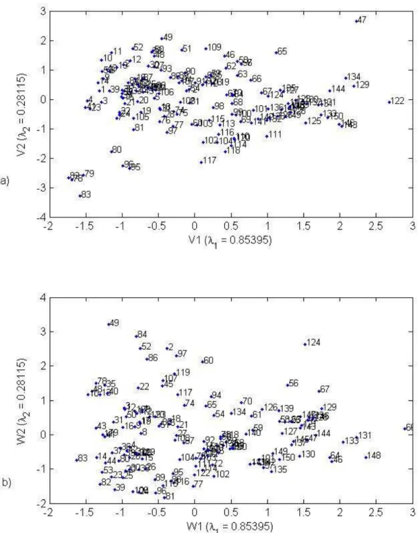
 ≤   =_ ≤ ≤   _≥  (23) 1 with d₂>d₁> . 0 2 3

Special cases 1 and 2 along with the general depth-based approach are illustrated in Figure 1. 4

5 6

4. Case study

7

In this section, the approach proposed in Section 3 is applied on a real world data set and 8

its performance is compared to that of the CCA approach. The case study on which the 9

comparison is carried out concerns the hydrometric station network of the southern part of the 10

province of Quebec, Canada. To be selected, each station in the data set must have a flood record 11

of at least 15 years of data and its historical data must be homogenous, stationary and 12

independent. The area of these catchments is larger than 200 km2 and less than 100 000 km2. 13

Finally, a total of 151 stations located between the 45o N and the 55o N are selected. The 14

geographical location of these stations is shown in Figure 2. 15

16

The variable selection is based on a previous study by Chokmani and Ouarda (2004). The 17

selected variables are of three types: physiographical, meteorological, and hydrological. The 18

physiographical variables are: basin area (AREA), mean basin slope (MBS) and the fraction of 19

the basin area covered with lakes (FAL). The meteorological variables are annual mean total 20

precipitation (AMP) and annual mean degree days over 0o C (AMD). The hydrological variables 1

are represented by at-site flood quantiles QT corresponding to a return period T. 2

3

The data bases used in the present study and the at-site frequency analysis are presented in 4

Kouider et al. (2002). The at-site flood frequency procedure includes the use of statistical tests of 5

hypothesis to test for homogeneity, independence and stationarity, the fitting of several statistical 6

distributions to the station data, and the use of goodness-of-fit tests to identify the most 7

appropriate distribution for each station. It is important to mention that the approach proposed in 8

the present paper does not require the use of a unique regional distribution. It is hence possible to 9

use a different (most appropriate) distribution in each station. For more details concerning the at-10

site frequency analysis, the reader is referred to Kouider et al. (2002). 11

12

Eaton et al. (2002) reported that, when modeling the physical mechanism of drainage 13

systems, scale effect should be eliminated from experiment data since it may have a negative 14

impact on the results. To reduce the scale effect, flood quantiles QT are standardized by the basin 15

area to obtain specific quantiles QST =QT AREA. In this study, the 10-year (QS10) and the 16

100-year (QS100) specific flood quantiles are selected. The basic statistics of these variables are 17

summarized in Table 1. 18

19

CCA application requires all variables to be transformed in order to be normalized and 20

standardized. The appropriate normalizing transformations for the present data set were obtained 21

by Chokmani and Ouarda (2004). A logarithmic transformation was used for the variables QS10, 22

CCA procedure is applied with values of the coefficient

α

ranging in the interval [0, 1]. An 1

optimal value of the coefficient

α

is selected according to minimum values of the relative bias 2

(RB) and the relative root mean square error (RRMSE) of the jackknife resampling procedure as 3

explained in Ouarda et al. (2001). The optimal value is found to be α =0.25 for the present case 4

study. The scatter plots of sites in the hydrological canonical space (W1,W2) and the physio-5

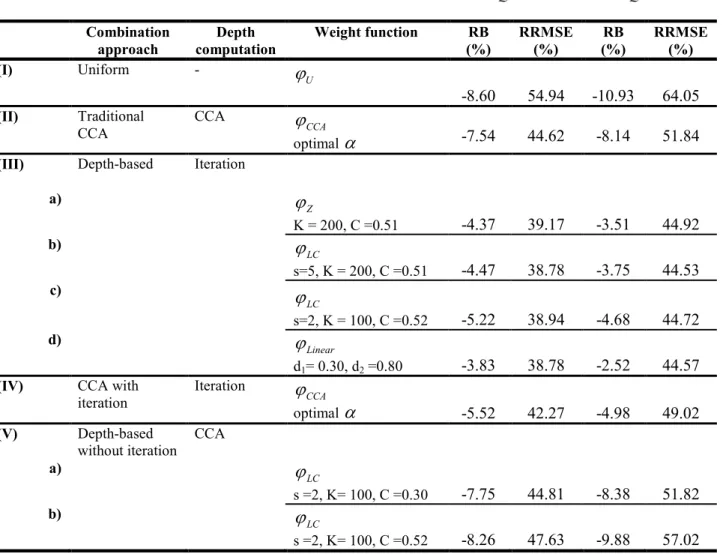
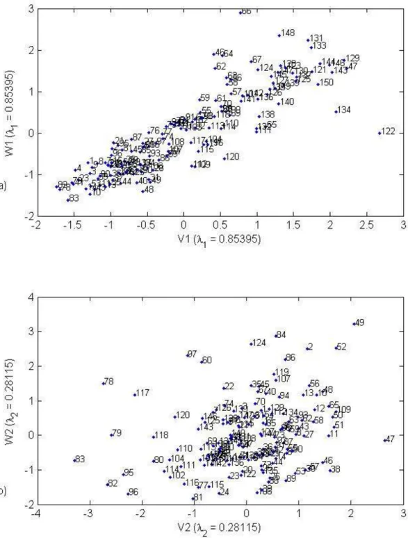
meteorological canonical space (V1,V2) are illustrated in Figure 3. 6 7 8 9

5. Study methodology

10

The proposed depth-based approach described in Section 3 is applied to the above case 11

study, and is compared to the CCA approach. Other methods are also considered in the 12

comparison. 13

14

From equation (16), it can be seen that the depth computation method and the weight 15

function are the two main elements of the estimation in the proposed approach. The depth can be 16

computed in two ways: by the CCA Mahalanobis distance using directly equation (10) in 17

equation (6); or by the iterative algorithm described in Section 3. Equation (6) indicates that the 18

Mahalanobis depth and Mahalanobis distance are equivalent, that is, their values can be deduced 19

from each other. Various combinations of depth computation and weight selection methods are 20

considered in this study. The following methods are compared: 21

I. The uniform approach which uses all sites with the same importance. 22

II. The traditional CCA approach considered with the optimal value of

α

. 23

III. The depth-based approach considered with the following weight functions: 1 a.

ϕ

_Z with K = 200 and C = 0.51. 2 b.

ϕ

_LC with s = 5, K = 200 and C = 0.51. 3 c.

ϕ

LC with s = 2, K = 100 and C = 0.52. 4

d.

ϕ

_Linear with d1 = 0.30 and d2 = 0.80.

5

IV. The CCA approach with iteration: It consists in the combination of the weight function 6

CCA

ϕ

with the optimal value of α =0.25 along with the Mahalanobis depth 7

evaluated by the iterative algorithm. This combination can be seen as a special 8

case of (III) with the specific weight function

ϕ

_CCA. 9

V. The depth-based approach without iteration: The depth is evaluated from the CCA 10

Mahalanobis distance using equation (10). The weight function is

ϕ

LC with the 11

following coefficients: 12

a. s = 2, K = 100 and C = 0.30, which is similar in shape to

ϕ

_CCAwith α =0.25. 13

b. s = 2, K = 100 and C = 0.52, which is one of the weight functions 14

considered in (III). 15

16

The combinations (IV) and (V) are introduced to study the effect of the depth evaluation method 17

and the weight function selection. The considered combinations are summarized in the left-hand 18

part of Table 2 and the corresponding weight functions are illustrated in Figure 4. 19

20

In order to evaluate the performance of the various methods, a jackknife resampling 21

temporarily from the region. The criteria employed to evaluate the performances of the 1

approaches are the relative bias (RB) and the relative root mean square error (RRMSE) given 2 respectively by: 3 1 ˆ 1 N i i i i y y RB N = y  −  = _{ }  

∑

(24) 4 2 1 ˆ 1 1 N i i i i y y RRMSE N = y  −  = _{ } −

∑

_{ } (25) 5

where y are the local realizations of the hydrological variable, ˆi y are the regional estimates and i 6

N is the number of sites in the data set.

7 8

6. Results and discussion

9

Results related to the various methods are summarized in Table 2. For all methods, results 10

indicate that the RB and RRMSE are smaller for QS10 than QS100. Generally in frequency 11

analysis, QST is more accurately estimated than QST’ if T < T’ since for small return periods, the 12

corresponding quantile is close to the central body of the distribution. Hence, an important part of 13

the data contributes to its estimation. Table 2 shows also that the results of the uniform method (I) 14

are the worst. This confirms the need to use regional delineation techniques. The remaining 15

methods are classified according to the depth evaluation procedure (iteration or direct CCA). The 16

iterative depth evaluation leads to better results than the direct evaluation using CCA. Indeed, the 17

results of the depth-based approach (III) are the best, and are followed by those of method (IV). 18

In these two methods the depths are iteratively evaluated. Moreover, the differences in terms of 19

RB and RRMSE are not significant between the various combinations in (III). 20

In methods (II) and (V), depths are evaluated directly using the CCA Mahalanobis 1

distance. These methods lead to RB and RRMSE values that are larger than those obtained by 2

methods (III) and (IV). In particular, the RB and RRMSE of methods (II) and (V) are 3

significantly larger than those of methods (III). The RB and RRMSE of (IV) are slightly smaller 4

than those of (II). In these last two methods, the same weight function

ϕ

_CCA is used. Hence, the 5

CCA approach results can be slightly improved when depths are iteratively evaluated. However, 6

the results from (V.b) are not satisfactory compared to the other methods except the uniform one 7

(I). Note that combination (V.b) uses the same weight function than (III.c). Note also that the 8

results of combinations (V.a) and (II) are very similar. In both these methods the depth is 9

evaluated using the CCA Mahalanobis distance and the corresponding weight functions have 10

similar shapes (see Figure 4). The results of combination (III.d) and the shape of the 11

corresponding weight function

ϕ

_Linearsuggest classifying the gauged sites into three classes: a 12

class of sites to be excluded from the regional estimation procedure; another class of 13

“intermediate” sites for which the contribution is gradually employed; and a last class of sites to 14

be fully included in the estimation. 15

16

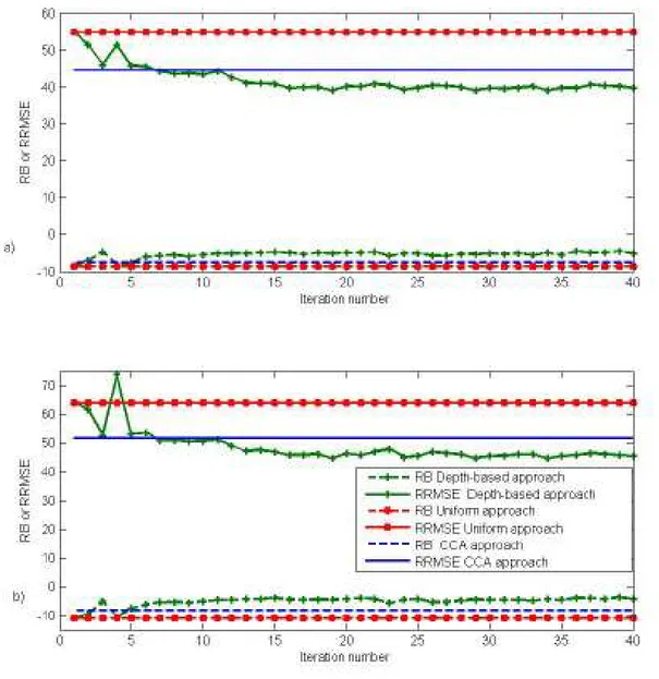
In the following, selected detailed results are presented. Figure 5 presents the evolution of 17

the performance criteria as a function of the iteration number for methods (I), (II) and (III.c). For 18

the uniform (I) and the traditional CCA (II) approaches, the criteria are represented by straight 19

lines, since they are independent of the iteration number. For both QS10 and QS100, the criteria 20

values of method (III.c) improve with the iteration number. Moreover, they seem to converge, 21

after approximately 15 to 20 iterations, to the corresponding results given in Table 2. This 22

that the computer running time of all the 40 iterations of (III.c) is comparable to that of the 1

traditional CCA approach. 2

3

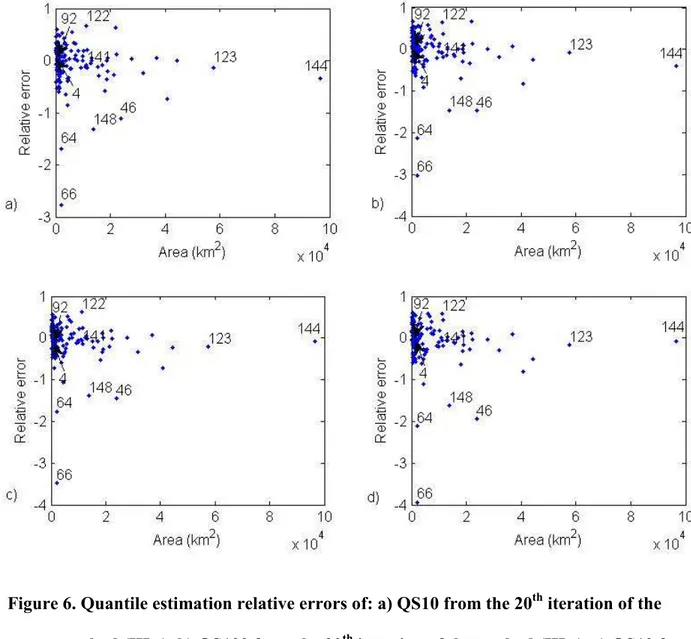
Figure 6 presents, for each site i, the relative error

(

y_i − yˆ_i

)

y_irelated to the estimation 4

of the specific quantiles QS10 and QS100 with respect to the basin area. It concerns the results of 5

the CCA approach (II) and those of the 20th iteration of the depth-based approach (III.c). The 20th 6

iteration is selected, as an example, since the criteria converge after 15 to 20 iterations. Using 7

both estimation methods, large negative errors are observed for some sites such as number 46, 64, 8

66 and 148. In particular, sites 64 and 66 have small basin areas. It is generally observed that the 9

relative errors obtained from the depth-based approach (III.c) are smaller than those obtained 10

from the traditional CCA approach (II). 11

12

The following two elements can be used to explain some aspects related to the CCA 13

approach: 14

1. Under the normality condition imposed on X and Y, it is implicitly assumed that the 15

conditional canonical variable

(

W V| =v₀

)

is N

(

Λv I₀, _p − Λ , see Ouarda et al. (2001). 2

)

16 Consequently: 17

(

0

)

0 E W V| =v = Λv and Var

(

W V| =v0

)

=Ip− Λ2 (26) 18

which suggests modeling the relationship between W and V by a linear regression model 19 as follows: 20 , W = Λ +V

ε

with

ε

~N

(

0,Ip− Λ 2

)

(27) 21

Usually, in the CCA approach, sites are presented in the hydrological canonical space 22

canonical spaces (V1,W1) and (V2,W2). This is illustrated in Figure 7 for the considered 1

data set. It shows that the relationship between V1 and W1 can be acceptably considered 2

to be linear, and hence meets the model (27), whereas it is not the case for V2 and W2. 3

The illustration in the space (V1,W1) is useful to get prior information about the 4

estimation error for a given site. 5

2. The canonical hydrological value W of the target-site is unknown. Hence, in the CCA ₀

6

approach, the Mahalanobis distance (10) is computed with respect to its expectation Λ v₀

7

(it represents also its estimator using (27)). This influences the computation of the 8

Mahalanobis distance, especially when the Mahalanobis distance 9

(

)

2 1

(

)

0 0 ( p ) 0 0

W − Λv ′ I − Λ − W − Λv between W and ₀ Λ is large. This is the case, for v₀

10

instance, for site number 66. 11

12

Figure 8 illustrates the Mahalanobis depths evaluated from (II) and from the 20th 13

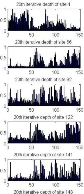
iteration of (III.c) for a selection of sites. The sites considered in Figure 8 are selected from 14

Figures 6 and 7 to represent a wide variety of conditions. Indeed, from Figure 6, sites number 66, 15

122 and 148 are estimated with very high relative errors. These sites are located far from the 16

straight line relating V1 and W1 as shown in Figure 7.a. However, sites number 4, 92 and 141 are 17

accurately estimated as shown in Figure 6 and they are located near the regressive line in Figure 18

7.a. Figure 8 shows that the global shapes of the depth values by both methods are similar. 19

However, differences in depth magnitude are observed, especially for site 122. This site has a 20

very high value of basin area covered with lakes (FAL = 43%). 21

From the above results and analysis it appears that the first important element, for 1

quantile regression estimation, is the accurate computation of depth values. The second important 2

element is related to the selection of the weight function. Hence, the results of the classical 3

delineation can be improved with accurate depth values (combination IV). However, generally 4

less accurate depth values with an arbitrary weight function can not improve the classical results 5

(combinations V). Consequently, the best combination of these two elements is a smooth weight 6

function along with an iteratively evaluated Mahalanobis depth (combinations III). 7

8

7. Conclusions and future research directions

9

The present paper provides an adaptation of the statistical notion of “depth function” in 10

regional flood frequency analysis. The depth-based approach is introduced in order to overcome 11

some drawbacks of the classical methods and to improve their performances. Along with the 12

flexibility and generality of the proposed method, it is shown that its use leads to improvements 13

in traditional methods. Furthermore, the proposed methodology can be useful in other areas and 14

disciplines of water resources where the regression model is applicable. 15

16

Introducing the statistical notion of depth function in regional flood frequency analysis 17

leads to several directions for future work including the following: 18

− The determination of an optimal weight function remains an element to be developed. One 19

option is to restrict the optimization problem to a specific parametric class of weight 20

functions, such as

ϕ

_LC or

ϕ

_Linear. Then, according to the optimal value of the considered 21

criterion, the coefficients of the weight function can be obtained. More flexible S-shaped 22

weight functions (such as the Gompertz function) represent a promising class to be 1

considered for optimization. 2

− The estimation in the index flood model (Dalrymple, 1960) should be developed following a 3

similar approach to the regression model. A comparison to the region of influence approach 4

(Burn, 1990) is to be considered. Note that the region of influence approach uses special 5

weight functions. 6

− In the present paper, the Mahalanobis depth function is considered for its simplicity and its 7

link to the CCA approach. It is of interest to consider other depth functions and to compare 8

the corresponding results. Note that Lin and Chen (2006) presented an estimator that is 9

similar to the one given by equation (16) using the projection depth function (equation 4). 10

They studied its asymptotic properties, including consistency, normality and robustness. 11

− The estimation of the uncertainty associated to regional quantiles represents an important 12

topic that is not often treated in the literature. It would be of value, in future efforts, to study 13

the uncertainty associated to the approach proposed in the present paper. It is important to 14

mention that some of the methods in the literature (such as Generalized and Weighted least 15

squares approaches) allow to carry out an analysis of the uncertainty (see e.g. Madsen and 16

Rosbjerg, 1997). However, with these approaches, the estimation of the uncertainty of the T-17

year event represents only the uncertainty on the regressive part without integrating the 18

uncertainty associated to the definition of the homogeneous regions. The depth-based method 19

does not suffer from this problem and hence it requires only one global uncertainty evaluation. 20

− Information concerning the spatial correlation between the various sites should be integrated 21

in the depth-based flood frequency procedure. 22

Acknowledgments

1

Financial support for this study was graciously provided by the Natural Sciences and 2

Engineering Research Council (NSERC) of Canada, and the Canada Research Chair Program. 3

The authors wish to thank the Editor in Chief, the Associate Editor and the two anonymous 4

reviewers for their useful comments which led to the improvement of the paper. 5

Bibliography

1

Arcones, M. A.; Chen, Z. and Giné, E. (1994) Estimators Related to U-Processes with 2

Applications to Multivariate Medians: Asymptotic Normality. Ann. Statist., 22, 1460-1477. 3

Alila, Y. (1999) A hierarchical approach for the regionalization of precipitation annual maxima in 4

Canada. J. Geophys. Res., 104, 31,645-31,655. 5

Alila, Y. (2000) Regional rainfall depth-duration-frequency equations for Canada. Water Resour. 6

Res., 36, 1767-1778.

7

Burn, D. H. (1990) Evaluation of regional flood frequency analysis with a region of influence 8

approach. Water Resour. Res., 26, 2257-2265. 9

Caplin, A. and Nalebuff, B. (1988) On 64%-majority rule. Econometrica, 56, 787-814. 10

Caplin, A. and Nalebuff, B. (1991a) Aggregation and social choice: A mean voter theorem. 11

Econometrica, 59, 1-23.

12

Caplin, A. and Nalebuff, B. (1991b) Aggregation and imperfect competition: On the existence of 13

equilibrium. Econometrica, 59, 25-59. 14

Chebana, F. and Ouarda, T.B.M.J. (2007) Multivariate L-moment homogeneity test. Water 15

Resour. Res., 43, W08406, doi:10.1029/2006WR005639.

16

Chokmani, K. and Ouarda T.B.M.J. (2004) Physiographical space-based kriging for regional 17

flood frequency estimation at ungauged sites. Water Resour. Res., 40, W12514, doi: 18

10.1029/2003WR002983. 19

Dalrymple, T. (1960) Flood frequency methods. United States Geological Survey Water-Supply 20

Paper, 1543 A, 11-51.

21

Durrans, S. R. and Tomic, S. (1996) Regionalization of low-flow frequency estimates: an 22

Eaton, B.; Church, M. and Ham, D. (2002) Scaling and regionalization of flood flows in British 1

Columbia, Canada. Hydrol. Processes, 16, 3245– 3263. 2

Ghosh, A. K. and Chaudhuri, P. (2005) On Maximum Depth and Related Classifiers. Scand. J. 3

Statist., 32, 327–350.

4

GREHYS (1996a) Presentation and review of some methods for regional flood frequency 5

analysis. J. Hydrology, 186, 63-84. 6

GREHYS (1996b) Inter-comparison of regional flood frequency procedures for Canadian rivers. 7

J. Hydrology, 186, 85-103.

8

Hosking, J. R. M. and Wallis, J. R. (1993) Some statistics useful in regional frequency analysis. 9

Water Resour. Res., 29, 271-282.

10

Kouider, A., Gingras, H.; Ouarda, T. B. M. J.; Ristic-Rudolf, Z. and Bobée, B. (2002) Analyse 11

fréquentielle locale et régionale et cartographie des crues au Québec [In French], Rep. R-627-12

el, Eau, Terre, et Environ., INRS, Ste-Foy, Que., Canada. 13

Lin, L. and Chen, M. H. (2006) Robust estimating equation based on statistical depth. Statist. 14

Papers, 47, 263-278.

15

Liu, R. Y. (1990) On a notion of data depth based on random simplices. Ann. Statist., 18, 405-16

414. 17

Liu, R. Y. (1992) Data depth and multivariate rank tests. In L-l Statistics and Related Methods (Y. 18

Dodge, ed.) 279 294. North-Holland, Amsterdam. 19

Liu, R. Y. and Singh, K. (1993) A quality index based on data depth and multivariate rank tests. 20

J. Amer. Statist. Assoc., 88, 257-260.

21

Liu, R. Y. (1995) Control Charts for Multivariate Processes. J. Amer. Statist. Assoc., 90, 1380-22

1388. 23

Liu, R. Y.; Parelius, J. M. and Singh, K. (1999) Multivariate analysis by data depth: descriptive 1

statistics, graphics and inference, (with discussion and a rejoinder by Liu and Singh). Ann. 2

Statist., 27, 783-858.

3

Madsen, H. and Rosbjerg, D. (1997) Generalized least squares and empirical Bayes estimation in 4

regional partial duration series index-flood modeling. Water Resources Research, 33, 771-5

781. 6

Mahalanobis, P. C. (1936) On the generalized distance in statistics. Proc. Nat. Acad. Sci. India, 7

12, 49-55.

8

Massé, J.-C. (2004) Asymptotics for the Tukey depth process, with an application to a 9

multivariate trimmed mean. Bernoulli, 10, 1-23. 10

Miller, K. ; Ramaswami, S. ; Rousseeuw, P. ; Sellares, T. ; Souvaine, D. ; Streinu, I. and Struyf, 11

A. (2003) Efficient Computation of Location Depth Contours by Methods of Combinatorial 12

Geometry. Statistics and Computing, 13, 153-162. 13

Mizera, I. (2002) On depth and deep points: a calculus. Ann. Statist., 30, 1681–1736. 14

Mizera, I. and Müller, C. H. (2004) Location-Scale Depth (with discussion). J. Amer. Statist. 15

Assoc., 99, 949-966.

16

Muirhead, R. J. (1982) Aspect of Multivariate Statistical Theory. John Wiley, Hoboken, N. J. 17

Nguyen, V.-T.-V. and Pandey, G. (1996) A new approach to regional estimation of floods in 18

Quebec. In: Delisle, C.E., Bouchard, M.A. (Eds.), Proceedings of the 49th Annual 19

Conference of the CWRA, June 26–28, Quebec City. Collection Environnement de l'U. de 20

M., 587–596. 21

Oja, H. (1983) Descriptive statistics for multivariate distributions. Statist. Probab. Lett., 1, 327-22

Ouarda, T. B. M. J. and Ashkar, F. (1994) Regional multiple regression flood frequency 1

estimation by the Peaks-Over-Threshold method. Internal Report, Department of 2

Mathematics, University of Moncton, Moncton, New Brunswick, Canada, Research report 3

for the Strategic Grant No. STR0118482 of NSERC, 20 pp. 4

Ouarda, T. B. M. J.; Haché, M.; Bruneau, P. and Bobée, B. (2000) Regional Flood Peak and 5

Volume Estimation in a Northern Canadian Basin. ASCE J. Cold. Reg. Engrg., 14, 176-191. 6

Ouarda, T. B. M. J.; Girard, C.; Cavadias, G. S. and Bobée, B. (2001) Regional flood frequency 7

estimation with canonical correlation analysis. J. Hydrology, 254, 157-173. 8

Ouarda, T. B. M. J.; Cunderlik, J. M.; St-Hilaire, A.; Barbet, M.; Bruneau, P.; Bobée, B. (2006) 9

Data-based comparison of seasonality-based regional flood frequency methods. J. 10

Hydrology, 330, 329-339.

11

Rencher, A. C. (2002) Methods of multivariate analysis. Second edition. Wiley Series in 12

Probability and Statistics. John Wiley & Sons, New York. 13

Rousseeuw, P. J. and Hubert, M. (1999) Regression depth. J. Amer. Statist. Assoc., 94

,

389-433. 14

Stedinger, J.R. and Tasker, G. (1986) Regional hydrologic analysis, 2, Model-error estimators, 15

estimation of sigma and log Pearson type 3 distributions. Water Resour. Res., 22, 1487-16

1499. 17

Tukey, J. (1975) Mathematics and picturing data. In Proceedings of the 1975 International 18

Congress of Mathematics, 2, 523-531.

19

van der Vaart, A.W. (1998) Asymptotic statistics. Cambridge Series in Statistical and 20

Probabilistic Mathematics. Cambridge University Press, Cambridge. 21

Zuo, Y. and Serfling, R. (2000) General notions of statistical depth function. Ann. Statist., 28 22

461–482. 23

Zuo, Y.; Cui, H. J. and Young, D. (2004) Influence function and maximum bias of projection 1

depth bused estimators. Ann. Statist., 32, 189-218. 2

Zuo, Y. and Cui, H. (2005) Depth weighted scatter estimators. Ann. Statist., 33, 381–413. 3

Table 1. Descriptive statistics of hydrological, physiographical and meteorological variables

1

Variable Unit Min Mean Max Standard

deviation MBS % 0.96 2.43 6.81 0.99 FAL % 0.00 7.72 47.00 7.99 AMP mm 646 988 1534 154 AMD degree-day 8589 16346 29631 5382 AREA km2 208 6255 96600 11716 QS10 m3/s.km2 0.03 0.22 0.53 0.13 QS100 m3/s.km2 0.03 0.31 0.94 0.20 2

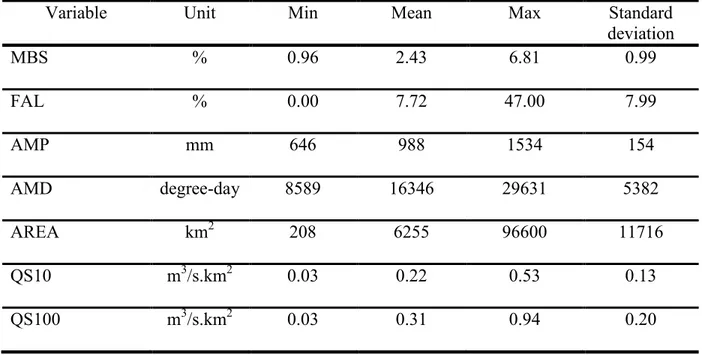
Table 2. Quantile estimation results with the various methods 1 2 QS10 QS100 Combination approach Depth computation Weight function RB (%) RRMSE (%) RB (%) RRMSE (%) (I) Uniform - U

ϕ

-8.60 54.94 -10.93 64.05 (II) Traditional CCA CCA CCA

ϕ

optimal

α

-7.54 44.62 -8.14 51.84

(III) Depth-based Iteration

a) Z

ϕ

K = 200, C =0.51 -4.37 39.17 -3.51 44.92 b) LC

ϕ

s=5, K = 200, C =0.51 -4.47 38.78 -3.75 44.53 c) LC

ϕ

s=2, K = 100, C =0.52 -5.22 38.94 -4.68 44.72 d) Linear

ϕ

d1= 0.30, d2 =0.80 -3.83 38.78 -2.52 44.57

(IV) CCA with

iteration Iteration CCA

ϕ

optimal

α

-5.52 42.27 -4.98 49.02 (V) Depth-based without iteration CCA a) LC

ϕ

s =2, K= 100, C =0.30 -7.75 44.81 -8.38 51.82 b) LC

ϕ

s =2, K= 100, C =0.52 -8.26 47.63 -9.88 57.02 3

1

Figure 1. Illustration of different regionalization approaches with the corresponding weight

2 functions 3 Neighborhood , 2 , 1 1 p p C_α α χ = + 1 Depth Weight Uniform Traditional CCA General new approach 1 0 Target site

1

Figure 2. Geographical location of the studied sites in the province of Quebec, Canada

2 3

1

Figure 3. Data set in the canonical spaces (a) physio-meteorological (b) hydrological

2 3

1

Figure 4. Weight functions used in the comparative study

2 3

1

Figure 5. RB and RRMSE using the uniform (I), the CCA (II) and the depth-based (III.c)

2

methods for the estimation of (a) QS10 and (b) QS100

1

Figure 6. Quantile estimation relative errors of: a) QS10 from the 20th iteration of the

2

method (III.c), b) QS100 from the 20th iteration of the method (III.c), c) QS10 from

3

the CCA method (II), d) QS100 from the CCA method (II). Selected sites are

4

indicated by their respective numbers

5 6

1

Figure 7. Scatter plot of the data set in the canonical spaces (V1,W1) and (V2,W2)

2 3

1

Figure 8. Depth values from the traditional CCA (II) and from the 20th iteration of the