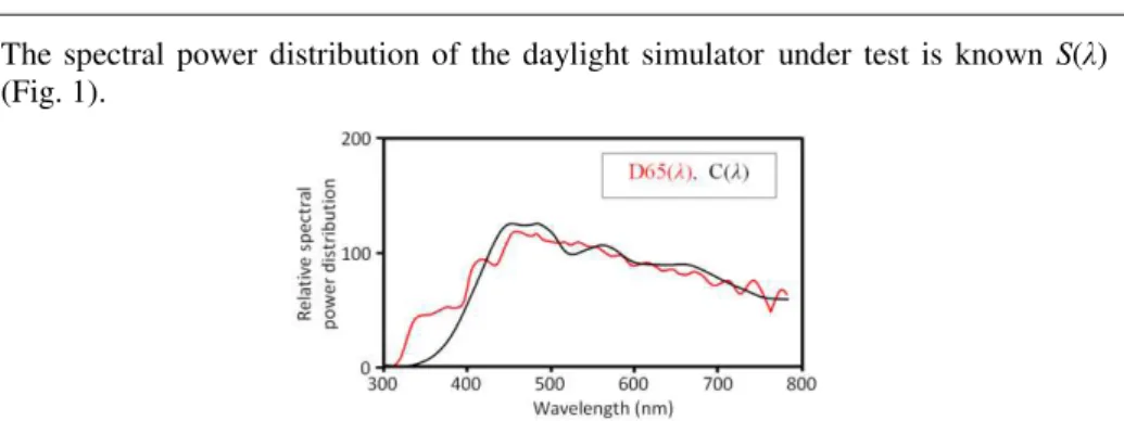
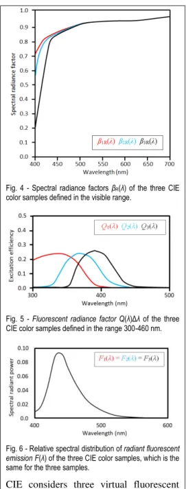
colour in the urban environment: a tool for the chromatic analysis of spatial coherence

Texte intégral

(1)Colour and Colorimetry Multidisciplinary Contributions Vol. XII B Edited by Davide Gadia. www.gruppodelcolore.it Regular Member AIC Association Internationale de la Couleur.

(2) Colour and Colorimetry. Multidisciplinary Contributions. Vol. XII B Edited by Davide Gadia – Dip. di Informatica – Università degli Studi di Milano Layout by Davide Gadia ISBN 978-88-99513-04-7 © Copyright 2016 by Gruppo del Colore – Associazione Italiana Colore Piazza C. Caneva, 4 20154 Milano C.F. 97619430156 P.IVA: 09003610962 www.gruppodelcolore.it e-mail: redazione@gruppodelcolore.it Translation rights, electronic storage, reproduction and total or partial adaptation with any means reserved for all countries. Printed in the month of October 2016.

(3) Colour and Colorimetry. Multidisciplinary Contributions Vol. XII B Proceedings of the 12th Conferenza del Colore Joined meeting with: AIDI Associazione Italiana di Illuminazione Colour Group Great Britain (CG-GB) Centre Français de la Couleur (CFC-FR) Colourspot (Swedish Colour Centre Foundation) Comité del color (Sociedad Española de Óptica) Groupe Français de l'Imagerie Numérique Couleur (GFINC) Politecnico di Torino Turin, Italy, September 08-09, 2016 Organizing Committee. Program Committee. Davide Gadia Anna Marotta Roberta Spallone. Alessandro Farini Massimiliano Lo Turco Veronica Marchiafava Marco Vitali. Organizing Secretariat Veronica Marchiafava – GdC-Associazione Italiana Colore Marco Vitali – Politecnico di Torino.

(4) Scientific Committee – Peer review Chiara Aghemo | Politecnico di Torino, IT Antonio Almagro | Escuela de Estudios Árabes, ES Fabrizio Apollonio | Università di Bologna, IT John Barbur | City University London, UK Cristiana Bedoni | Università degli Studi Roma Tre, IT Laura Bellia | Università degli Studi di Napoli Federico II, IT Giordano Beretta | HP, USA Berit Bergstrom | NCS Colour AB, SE Giulio Bertagna | B&B Colordesign, IT Janet Best | Colour consultant, UK Marco Bevilacqua | Università di Pisa, IT Fabio Bisegna | Sapienza Università di Roma, IT Aldo Bottoli | B&B Colordesign, IT Patrick Callet | École Centrale Paris, FR Jean-Luc Capron | Université Catholique de Louvain, B Antonella Casoli | Università di Parma, IT Céline Caumon | Université Toulouse2, FR Vien Cheung | University of Leeds, UK Michel Cler | Atelier Cler Études chromatiques, FR Osvaldo Da Pos | Università degli Studi di Padova, IT Arturo Dell'Acqua Bellavitis | Politecnico di Milano, IT Hélène De Clermont-Gallerande | Chanel Parfum beauté, FR Julia De Lancey | Truman State University, Kirsville-Missouri, USA Reiner Eschbach | Xerox, USA Maria Linda Falcidieno | Università degli Studi di Genova, IT Patrizia Falzone | Università degli Studi di Genova, IT Renato Figini | Konica-Minolta, IT Agnès Foiret-Collet | Université Paris1 PanthéonSorbonne, FR Marco Frascarolo | Università La Sapienza Roma, IT Davide Gadia | Università degli Studi di Milano, IT Marco Gaiani | Università di Bologna, IT Anna Gueli | Università di Catania, IT Robert Hirschler | Serviço Nacional de Aprendizagem Industrial, BR Francisco Imai | Canon, USA Muriel Jacquot | ENSAIA Nancy, FR Kay Bea Jones | Knowlton School of Architecture, Ohio State University, USA Marta Klanjsek Gunde | National Institute of Chemistry- Ljubljana,SLO Guy Lecerf | Université Toulouse2, FR Massimiliano Lo Turco | Politecnico di Torino, IT. Maria Dulce Loução | Universidade Tecnica de Lisboa, P Lia Luzzatto | Color and colors, IT Veronica Marchiafava | IFAC-CNR, IT Gabriel Marcu | Apple, USA Anna Marotta | Politecnico di Torino IT Berta Martini | Università di Urbino, IT Stefano Mastandrea | Università degli Studi Roma Tre, IT Louisa C. Matthew | Union College, SchenectadyNew York, USA John McCann | McCann Imaging, USA Annie Mollard-Desfour | CNRS, FR John Mollon | University of Cambridge, UK Claudio Oleari | Università degli Studi di Parma, IT Sonia Ovarlez | FIABILA SA, Maintenon, FR Carinna Parraman | University of the West of England, UK Laurence Pauliac | Historienne de l'Art et de l'Architecture, Paris, FR Giulia Pellegri | Università degli Studi di Genova, IT Luciano Perondi | Isia Urbino, IT Silvia Piardi | Politecnico di Milano, IT Marcello Picollo | IFAC-CNR, IT Angela Piegari | ENEA, IT Renata Pompas | AFOL Milano-Moda, IT Fernanda Prestileo | ICVBC-CNR, IT Boris Pretzel | Victoria & Albert Museum, UK Paola Puma | Università degli Studi di Firenze, IT Noel Richard | University of Poitiers, FR Katia Ripamonti | University College London, UK Alessandro Rizzi | Università degli Studi di Milano, IT Maurizio Rossi | Politecnico di Milano, IT Michela Rossi | Politecnico di Milano, IT Elisabetta Ruggiero | Università degli Studi di Genova, IT Michele Russo | Politecnico di Milano, IT Paolo Salonia | ITABC-CNR, IT Raimondo Schettini | Università degli Studi di Milano Bicocca, IT Verena M. Schindler | Atelier Cler Études chromatiques, Paris, FR Andrea Siniscalco | Politecnico di Milano, IT Roberta Spallone | Politecnico di Torino, IT Christian Stenz | ENSAD, Paris, FR Andrew Stockman | University College London, UK Ferenc Szabó | University of Pannonia, H Delphine Talbot | University of Toulouse 2, FR Raffaella Trocchianesi | Politecnico di Milano, IT Stefano Tubaro | Politecnico di Milano, IT Francesca Valan | Studio Valan, IT Marco Vitali | Politecnico di Torino, IT Alexander Wilkie | Charles university Prague, CZ.

(5) Organizers:. Patronages:.

(6) Index. 1. COLOUR AND MEASUREMENT / STRUMENTATION………………………………..……..9 The Self-luminous Neutral Scale in the OSA-UCS system and Whittle’s Formula 11 C. Oleari, M. Melgosa Evolution of colours in football shirts through colorimetric measurements: Fiorentina's case 19 A. Farini, E. Baldanzi, M. Raffaelli, F. Russo A natural method to describe colours under different light sources 27 O. da Pos, P. Fiorentin. 2. COLOUR AND DIGITAL …………………………………………………………...…………. 39 . Random Spray Retinex and its variants STRESS and QBRIX: Comparison and Experiments on Public Color Images 41 M. Lecca, A. Rizzi , G. Gianini A technique to ensure color fidelity in automatic photogrammetry 53 M. Gaiani, F. I. Apollonio, A. Ballabeni, F. Remondino Photometric and photorealistic representation of luminaires in 3D software 67 A. Siniscalco, G. Guarini. 3. COLOUR AND LIGHTING ……………………………………………………………………79 Warm white, neutral white, cold white: the design of new lighting fixtures for different working scenarios 81 D. Casciani, F. Musante, M. Rossi Daylight-simulator evaluation by “Special metamerism index: change in illuminant” (Computer program) 93 G. Simone, C. Oleari Unified Profiles of Spectral Data to support Spatial and Dynamic Color Designs 103 M. Reisinger 6.

(7) The experience of equivalent luminous colors at architectural scale 109 U. Besenecker, T. Krueger, J. Bullough, Z. Pearson, R. Gerlach. 4. COLOUR AND PSYCHOLOGY ………………………………………………………….……119 Variational achromatic induction and beyond 121 G. Gronchi, E. Provenzi LED light scenes for artworks colour perception 129 L. Bellia, F. Fragliasso, E. Stefanizzi The Impact of Color on Increasing Self-Confidence among People with Multiple Sclerosis Disease 141 B. Abdollahi Gohar, M. Khalili From artistic expression to scientific analysis of color texture 151 A. Bony, L. Noury, C. Fernandez-Maloigne. 5. COLOUR AND RESTORATION ………………………………………………………….…163 The color of fluorescence: non-invasive characterization of fluorescent pigments used in contemporary art 165 M. Gargano, L. Bonizzoni, L. Cerami, S. Francone, N. Ludwig Innovative methods for a recognizable gold leaf integration 173 R. Capezio, T. Cavaleri, G. Piccablotto, M. Pisani, P. Triolo, M. Zucco Diagnostic study on original stamps of the Kingdom of Sardinia 185 T. Cavaleri, A. Conte, A. Piccirillo. 6. COLOUR AND BUILT ENVIRONMENT ……………………………………………………..197 Colour, Shape and Pattern on New Shading Façades 199 A. Premier Questioning Mediterranean white 207 M. P. Iarossi, C. Pallini Colour in the urban environment: a tool for the chromatic analysis of spatial coherence 219 L. Nguyen, J. Teller Contemporary residential streetscape: how colors and material differ from the traditional streetscape. A case study in Tokyo 231 L. Alessio Chromatic experiences: from the territory to the industry 243 L. Perdomo 7.

(8) 7. COLOUR AND DESIGN ……………………………………………………………………….255 Repetition of Color in the Nubian painting 257 S. Ahmed Ibrahim , H. Ahmed Ragab Impressionist style in the design for printing women clothes fabric 269 A. H. F. Sanad Stability disruption of a nail polish shade 281 C. Pierron, D. Roger, G. Planeix, N. Baudouin, H. de Clermont-Gallerande Don't Poles like colors? 283 B. Groborz. 8. COLOUR AND CULTURE …………………………………….………………………………295 Colour as a continuous protagonist of the multidimensionality of plastic languages –“Invited Paper” 297 Á. García Codoner From Skeuomorphism to Material Design and back. The language of colours in the 2nd generation of mobile interface design 309 L. Bollini “Out of the blue Foam”. MVRDV’s Didden Village as a full-scale model 321 F. Colonnese Colour emotion of 15th and 16th centuries Ottoman Divan poetry 331 B. Ulusoy, M. Kalpaklı Color and history in designing containers inspired by “KolahFarangi” Building of “Mohtasham” Garden in Rasht city 339 L. Akbar Colour of residential architecture of classicism and neoclassicism in Russia 347 M. Komarova Sitting in a kitchen full of colours with Claude Monet and Carl Larsson 353 M. Ahlqvist-Juhlin, M. Moro. 9. COLOUR AND EDUCATION …………………………………….……………………………359 Using colors to teach children how to raise a plant 361 E. Atighi Lorestani, M. Khalili The effect of color perception on individual skills for children with autism 373 M. Khalili, T. Khodayarian, R. Fesharakifard. 8.

(9) 1. COLOUR AND MEASUREMENT / STRUMENTATION.. 9.

(10) 10.

(11) The Self-luminous Neutral Scale in the OSA-UCS system and Whittle’s Formula 1 1. Claudio Oleari, 2Manuel Melgosa. Università degli Studi di Parma, Dip. Fisica e Scienze della Terra, 43214 Parma, Italy _ claudio.oleari@fis.unipr.it 2 Universidad de Granada, Departamento de Óptica, 18071 Granada, Spain _ mmelgosa@ugr.es. 1. Introduction Every psychometric color space and perceived color system has an achromatic line defining a neutral scale spanned by a lightness coordinate, e.g., L* in CIELAB and CIELUV, LOSA in the OSA-UCS system, Munsell’s value V in the Munsell system and Dunkelstufe D in DIN 6264 system. These neutral scales can be used to calculate barely visible threshold changes of lightness, or equal-appearing suprathreshold steps of grey scale, matching grey appearances, etc. Currently, CIE TC 193 Calculation of Self-Luminous Neutral Scale is investigating to recommend a neutral scale for self-luminous surfaces [1], and hopefully the new recommendation may complement or help to replace the grey scales previously mentioned. This work considers the lightness scale of the OSA-UCS system [2-7], at the present defined by the complicate Semmelroth formula, with the intent of evaluating the simpler Whittle formula [8-10] for representing the OSA-UCS lightness. The contribution of this work is divided into two parts: 1) the fitting of the OSA-UCS achromatic scale by the Whittle formula as function of the percentage luminance factor Y10; 2) lightness scale in the OSA-UCS system: a) the definition of a percentage luminous factor W obtained by a fitting of the constant OSA-UCS lightness planes in the (LOSA, g, j) space by a linear mixing of the tristimulus values, as it is for the percentage luminance factor Y10; b) the evaluation of a relative spectral luminous-efficiency-function W(λ), in analogy with the relative spectral luminous efficiency function V10(λ), which takes into account the Helmholtz-Kohlrausch effect; c) the fitting of the neutral scale from Whittle’s formula, denoted by LW, as function of the percentage luminous factor W (A comparison is made between the LW, obtained from Whittle’s formula, and the original LOSA, obtained from Semmelroth’s formula); d) the evaluation of the metrics in the space (LW, GW, JW) by the Euclidean colordifference formula [11-13]. 2. OSA-UCS’ lightness formula The OSA-UCS system [2-4] is organized in planes with constant lightness and lightness LOSA is one of the coordinates that spans the OSA-UCS space. The color samples of the OSA-UCS atlas are observed on a grey background, i.e. a homogeneous area adjoining the target. Therefore it is found that the lightness LOSA. 11.

(12) 1) is positive if the luminance factor of the color sample is greater that the luminance factor of the grey surround, zero if equal and negative if lower; 2) the lightness LOSA takes into account the Helmholtz-Kohlrausch effect, according to which, in addition to luminance, chromaticity also contributes to the brightness; 3) the lightness LOSA takes into account the crispening effect, according to which the brightness of a sample is affected by the brightness of the grey surround, whose percentage luminance factor is Y10 = 30. All this is described by a formula given by the OSA-UCS Committee according to a modification of Semmelroth’s formula LOSA. 5.9(Y01/ 3. 2 C ) 14.4 3. 1 2. (1). where 1/ 3. C F. 0.042 Y0 30 for (Y0 30) 0 1/ 3 0.042 Y0 30 for (Y0 30) 0. with. Y0. Y10 F. (2). 4.4934 x102 4.3034 y102 4.2760 x10 y10 1.3744 x10 2.5643 y10 1.8103. and Y10 is a percentage luminance factor of the color sample. The Helmholtz-Kohlrausch effect is described by the factor F, which modifies the percentage luminance factor Y10. The factor F assumes an equal value on ellipses centered at (x10 = 0.3859, y10 = 0.4897), with a ratio between the axis lengths equal to 1.4138 and with the major axis forming with the axis x10 an angle of 43.73°. The value of F for the D65 chromaticity is 1, i.e. the illuminant D65 is assumed achromatic. 3. Whittle’s lightness formula Paul Whittle proposed a lightness formula for a self-luminous grey-scale as “the simplest and most precise” calculation of the change of luminance ΔY (in cd/m2) necessary to achieve any number of just noticeable differences (JNDs) of achromatic appearance ΔLW. [8-10] Whittle’s JNDs are calculated from the background luminance, Yb, of the increment or decrement ΔY. The luminance interval ΔY is defined as the difference between target luminance Y and Yb: Y Yb Yd Yb. JNDs between[Y ,Yb. Y ] a1 log10 1 b(1 k ). JNDs between[Y ,Yb. Y ] a2 log10 1 b(1 k ). (3). Yb Y k (Yb Y ) Yd Y. where b = 6.58, a1 = 8.22, a2 = –7.07, Yd = 0.39 cd/m2 is the dark light noise and k is a constant in the interval [0,1] to account for the effect of intraocular scattering, which grows as viewing angle subtended by target decreases.. 12.

(13) 4. Analysis restricted to only color samples of the OSA-UCS atlas considered as significant for an achromatic scale Since not all the constant lightness planes have an achromatic sample in the OSAUCS Atlas, the achromatic scale we are going to propose is obtained from the achromatic specimens, where exist, and by the average of the color specimens with |g|≤1, |j|≤1 elsewhere. These samples are considered as representative of an achromatic color scale in the OSA-UCS system. For these achromatic samples the Helmholtz-Kohlrausch effect is considered negligible and consequently the lightness is only function of the luminance factor Y10. The Whittle lightness formula in Eq. (3) is defined on an absolute scale while the OSA-UCS system is defined on a relative scale (accordingly, in next Equations the luminance will be substituted by the percentage luminance factor and the JNDs by the lightness). Therefore the constants of the Whittle formula have to be redefined for a relative scale. for Y10. Y10,b LW. a1 log10 1 b1. for Y10 Y10,b LW. a2 log10 1 b2. (Y10 Y10,b ). (4). (Y10,d Y10,b ) ( Y10 Y10,b ). (5). (Y10,d Y10 ). where Y10,b = 30 is the percentage luminance factor of the background and Y10,d is the dark light noise that is seen in the absence of any light. Equations (4) and (5) provide equal value for Y10 = Y10,b, i.e. for LOSA = 0. The constant k, present in Eq. (3), is supposed equal to 0 for the view of the size of the viewing angle of the OSAUCS samples. Next Whittle’s formula fitted the LOSA lightness data of the color specimens with |g| ≤ 1, |j| ≤ 1, assuming zero dark light noise and zero intraocular scattering,. for LOSA. 0 or Y10. Y10,b. 30 LW. 12.2359log10 1 1.1076. (Y10 30) 30. (6). for LOSA. 0 or Y10. Y10,b. 30 LW. 5.2406log10 1 2.9615. ( Y10 30) Y10. (7). with fitting RMS < 0.10 computed on the whole set of color specimens with |g| ≤ 1 and |j| ≤ 1 of the OSA-UCS atlas. Eqs. (6) and (7) regard only the achromatic scale. Figure 1. plots the Whittle function fitted on the OSA-UCS data, together the data given by the OSA-UCS atlas. 5. Analysis extended to the whole OSA-UCS atlas by fitting lightness with Whittle’s formula i) Spectral luminous efficiency function In a controlled visual situation adapted to the D65 illuminant with a color sample on a grey background, lightness depends only by the tristimulus values that specify the color sample and background. 13.

(14) LOSA LW 5. 0. –5. for Y10. 30 LW. 12.2359log10 1 1.1076. for Y10. 30 LW. 5.2406log10 1 2.9615. 10. (Y10 30) 30. ( Y10 30) Y10. 20 Y10,b = 30 40 50 60 Percentage luminance factor Y10. 70. Fig. 1. Plot of the Whittle function (red line) over the data of the OSA-UCS atlas with |g|≤1, |j|≤1 represented by grey crosses (×). The big black dots (●) represent the average of the value of the data of the OSA-UCS atlas at equal lightness and the red dots (●) represent the value of the Whittle function averaged over the data of the OSA-UCS atlas with |g|≤1, |j|≤1 and equal lightness.. The loci with constant lightness are planes in the OSA-UCS space. The formula of Semmelroth describes the constant lightness loci with surfaces that are no longer planes in tristimulus space. This means that the lightness is a nonlinear function of the tristimulus values. The representation of the lightness by means of a linear function of the tristimulus values of the color sample is here considered as an approximation. As known the percentage luminance factor Y10 is the tristimulus value that represents the luminous stimulation. First, this analysis searches for fitting the lightness of the OSA-UCS system with a linear function of the tristimulus values of the color samples. As we will see, the obtained function is almost equal to each value of lightness and this leads us to believe that the linear fit is a good approximation. In analogy to the percentage luminance factor Y10, that is a coordinate in the tristimulus space, this linear approximation led us to define a percentage luminous factor W, representing a relative luminous stimulation in the OSA-UCS system that takes into account the Helmholtz-Kohlrausch effect in a linear approximation. 14.

(15) LY Y10. LZ Z10 with LX. 0.2152, LY. 0.7305, LZ. 0.0761. with LA. 0.4975, LB. 0.3487, LC. 0.1756. W. LX X10. W. LA A LB B LC C. (8). where (X10, Y10, Z10) and (A, B, C) are the tristimulus values in the X10Y10Z10 reference frame and in the adapted ABC reference frame [5-7], respectively, which are related by. A B C. 0.6597 0.4492 0.3053 1.2126. 0.1089 0.0927. 0.0374 0.4795. 0.5579. X 10 Y10 Z10. (9). On this basis, it is defined a relative spectral luminous efficiency function W(λ), in analogy with the relative luminous efficiency function V10(λ), which has a very low variation when lightness changes (Figure 2):. W( ). LX x10 ( ) LY y10 ( ) LZ z10 ( ) with LX. W( ). 0.7305, LZ. 0.0761. 0.3487, LC. 0.1756. (10). LA a ( ) LB b ( ) LC c ( ) with LA. where. 0.2152, LY. x10 ( ), y10 ( ), z10 ( ). 0.4975, LB and. a ( ), b ( ), c ( ). are the color-matching. functions in the X10Y10Z10 reference frame and in the adapted ABC reference frame, respectively. For an analysis of the spectral luminous efficiency function see references [14-18]. W(λ) 1. 0. 400. 500 600 Wavelength (nm). 700. Fig. 2. Relative spectral luminous efficiency functions obtained from the different lightness planes of the OSA-UCS system (grey lines) and relative spectral luminous efficiency function W(λ) (red dots ● and red line) computed as weighted average, with weights equal to the numbers of color samples belonging to any constant lightness plane .. 15.

(16) ii) Luminous factor and Whittle’s formula The LOSA lightness has been related to the percentage luminous factor W for each sample of the OSA-UCS system and the best fit of LW by using Whittle’s formula is shown in Figure 3.. LW LOSA 5. 0. –5. for W. for W. 10. 30 LW. 30 LW. (W 0.4 ( W 1 2.4190 0.4. 10.5548 log10 1 1.3270. 5.8178log10. 20 Wb = 30 40. 50. 60. 30) 30 30) W. 70. W. Fig. 3. Whittle’s function in Eqs. (11) (12) (red line) over the lightness data of the OSA-UCS atlas represented by grey crosses (×). The big black dots (●) represent the average of the value of the LOSA data at equal lightness and the cyan line represents the results from Semmelroth’s formula.. Whittle’s formula with best fitting parameters is: Wb. 30 LW. 10.5548log10 1 1.3270. (W 30) (0.4 30). with RMS. 0.12 (11). for W Wb. 30 LW. 5.8178log10 1 2.4190. ( W 30) (0.4 W ). with RMS. 0.15 (12). for W. where Wb = 30 corresponds to LOSA = 0 and is the percentage luminous factor of the grey background behind the color samples, and the dark light noise is approximated with a 0.4 value. The RMS value of these fits were computed on the whole OSAUCS atlas. The two fitted Eqs. (11) and (12) provide equal value for W = 30, i.e. LOSA = 0.. 16.

(17) iii) Metrics and Euclidean color-difference formula in the (LW, GW, JW) space with Whittle’s lightness The color-difference formulas have been long and deeply studied in recent decades and their study is not yet completed. The OSA-UCS space has been studied with considerable success to represent the color differences [11-13]. Here we consider the Euclidean color-difference formula ΔEE defined in the log-compressed space derived from space (LOSA, G, J) transferring this formula into the log-compressed space derived from space (LW, GW, JW) to assess its quality. The Euclidean formula depends on four parameters, which are defined on the experimental color difference data by an optimization process. The STRESS quantity [19] statistically quantifies the quality of these formulas. This operation is repeated in the new space (LW, GW, JW) by using the same experimental data used in the previous work [12] and STRESS = 28.42 is improved [STRESS = 29.48 in (LOSA,E, GE, JE)]. The transformations from the tristimulus space to (LW, GW, JW) space are as follows: 1) (A, B, C), W and LW are defined by Eqs. (8), (9), (11) - (12), respectively; 2) The coordinates (GW, JW) are defined by. JW GW. 2(0.5735LW 0. 7.0892). 0.1792 0.9482. 0 2(0.7640 LW 0.9837 0.3175. 9.2521). ln. A/ B 0.9366. ln. B/C 0.9807. (13). The Euclidean color-difference formula in (LW,E, GW,E, JW,E) is the following. EW ,E. (14). ( LW ,E )2 ( GW ,E )2 ( JW ,E )2. where. LW ,E. b 1 ln 1 L 10 LW bL aL. JW ,E. with aL. CW ,E sin(hW ), GW ,E. 2.8628 and bL. 0.0106. CW ,E cos(hW ). with. hW. CW ,E. arctan. b 1 ln 1 C 10CW bC aC. JW GW. with aC 1.2204 and bC. GW 2. CW. 17. JW 2 .. 0.0448.

(18) Bibliografia [1] http://www.cie.co.at/index.php/Technical+Committees. [2] MacAdam, D.L., Uniform color scales, J. Opt. Soc. Am. 64, 1691-1702 (1974). [3] MacAdam, D.L., Colorimetric data for samples of OSA uniform color scales, J. Opt. Soc. Am. 68, 121-130 (1978). [4] MacAdam, D.L., Color Measurement. Springer-Verlag, Berlin (1985), pp. 165-177. [5] Oleari, C.,Color Opponencies in the system of the uniform color scales of the Optical Society of America. J. Opt. Soc. Am. A 21, 677-682 (2004). [6] Oleari, C., Hypotheses for Chromatic Opponency Functions and their Performance on Classical Psychophysical Data, Color Res. Appl. 30, 31-41 (2005). [7] Oleari, C., Corresponding color datasets and a chromatic adaptation model based on the OSA-UCS system. J. Opt. Soc. Am. A 31, 1502-1514 (2014). [8] Whittle, P., Brightness, discriminability and the ‘Crispening Effect’, Vis Res. 32, 1493-1507 (1992) [9] Whittle, P., The psychophysics of contrast brightness, In A. Gilchrist (Ed.), Lightness, brightness, and transparency. Hillsdale: Erlbaum (1994). [10] Carter, R.C. & Brill M.H., Calculation of self-luminous neutral scale: How many neutral steps can you see on that display? J. Soc. For Info. Display 22, 177-186 (2014). [11] Huertas, R., Melgosa, M. and Oleari, C., Performance of a color-difference formula based on OSA-UCS space using small–medium color differences, J. Opt. Soc. Am. A 23, 2077-2084 (2006). [12] Oleari, C., Melgosa, M. and Huertas, R., Euclidean color-difference formula for small–medium color differences in log-compressed OSA-UCS space. J. Opt. Soc. Am. A 26, 121-134 (2009). [13] Oleari, C., Melgosa, M. and Huertas, R., Generalization of color-difference formulae for any illuminant and any observer by perfect color-constancy actuation in a color-vision model based on the OSA-UCS system. J. Opt. Soc. Am. A 28, 2226-2234 (2011). [14] Wyszecki, G., Correlate for brightness in term of CIE chromaticity coordinates and luminous reflectance, J. Opt. Soc. Am., 57, 254-257 (1967). [15] Kaiser, P.K., and Greenspon, T.S., Brightness Difference and Its Relation to the Distinctness of a Border, J. Opt. Soc. Am., 61, 962-965 (1971). [16] Ware, C., Cowan, W.B., Specification of heterochromatic brightness matches: A conversion factor for calculating luminances of stimuli that are equal in brightness. National research Council of Canada. 42 pages, Publication N° 26055 (1983). [17] Kaiser, P.K., CIE 1.03. Models of heterochromatic brightness matching. CIE Journal 5, 57-59 (1986). [18] Sève, R., Physique de la couleur, Masson, Paris (1996) [19] García, P. A., Huertas, R.., Melgosa, M., and Cui, G., Measurement of the relationship between perceived and computed color differences, J. Opt. Soc. Am. A 24,1823–1829 (2007).. 18.

(19) Evolution of colours in football shirts through colorimetric measurements: Fiorentina's case 1. Alessandro Farini, 1Elisabetta Baldanzi, 1Marco Raffaelli, 1Francesco Russo 1. CNR-Istituto Nazionale di Ottica alessandro.farini@ino.it, elisabetta.baldanzi@ino.it. 1. Introduction Football fans express their identification with their team especially with colours of football shirts. The respect of “tradition” is something so important that very small changes can provoke anger in fans, who express their opposition in news and social media. This could create problems for merchandising[1]. Fiorentina (Florence’s football team) wears purple shirts, very uncommon in football world[2]. Probably for this reason shirt’s colour is a very sensitive topic for Fiorentina’s fans (Fig.1).. Fig. 1 – A graffito “signed” by some Fiorentina’s supporters: the translation is “we say no to the bluish shirt”. In the recent years the introduction of high definition colour television and new strategy of merchandising have assigned an important role to shirt’s colour. Checking and the reproduction of official colours of a football team is nowadays very important. 2. Material and Methods Thank to the help of Museo Fiorentina[3] we have received at our lab 50 original shirts belonging to different sport seasons. Every shirt is called using the year of the second part of the season; as an example, the shirt used during the season 1958-1959 will bel called 1959. We have measured every shirt using a Minolta spectrophotometer Cm-2500c with 10 nm of resolution, 45°/0° geometry optics and 360-740 nm wavelength range. We have checked our measurements using, on three samples, a very accurate instrument: a Perkin Elmer spectrophotometer lambda 900 with an integrating sphere. The measurements of the two instruments agree within the experimental error: we decided to use Cm-2500c that permits to see the exact point of measurement. This peculiarity is very useful when we want to check shirts with different hues.. 19.

(20) Ageing is a real problem in this kind of measurements. Nowadays every shirt is used only one time but during the the 70’s and before every shirt could be used and washed many times during a season, producing a degradation in colours. Furthermore, old shirts could be inhomogeneous in colours: in order to check this hypothesis, we have measured the same shirt in ten different points apparently of the “same purple”. The results expressed in the CIELab system are shown in Tab.1. L a b. 25.1±0.7 27.9±0.7 -42.4±0.9. Tab. 1 – Mean and standard deviation obtained by ten measurements on the same shirt changing the measurement point.. 3. Experimental Results For every shirt we can examine the reflectance spectrum and the colour coordinates. Here we present only some data in order to present the variability trough years: a complete report will be published in the future together with some psychophysical measurements that want to investigate if every Fiorentina shirt could be called “purple” nowadays. In Fig.2 the reflectance spectra of 1959 (the oldest shirt available at Museo Fiorentina when we made the measurements) 1967, 1968, 1969, 1970 are shown. The first 4 shirts are very dark. This is a typical feature of the shirts in the “golden age” of Fiorentina (Fiorentina won the championship in 1955-1956 and 1968-1969): a radio show devoted to Fiorentina is called “Viola Scuro” (Dark Purple in Italian) in order to create a link with these famous years. The 1970 shirt is redder and less dark. 70. 60 1959 1967 1968 1969 1970. Reflectance (%). 50. 40. 30. 20. 10. 0 350. 400. 450. 500. 550 600 Wavelength (nm). 650. Fig. 2 – Reflectance spectra for 1959-1967-1968-1969-1970.. 20. 700. 750.

(21) Fig. 3 – Fiorentina’s shirt for season 1958-1959.. 1982 (Fig.4) is a very famous shirt for the history of Fiorentina because in that year many football team decided to renovate their shirt and their logo. Probably we can define 1982 as the first year of the “modern football”. The year before Fiorentina’s logo was completely renewed with an overlap between the traditional red fleur-de-lis and a capital "F", for Fiorentina. Supporters disliked it when it was introduced, but the logo remained until 1990. In the same year for the first time in Italy a sponsor name was allowed on the shirt.. Fig. 4 - Fiorentina’s shirt for season 1981-1982.. 1982 is the brightest shirt in Fiorentina history. Its difference is evident looking at Lightness, but also looking at reflectance spectra (Fig.5).. 21.

(22) 80. 70. 60 1959 1982 1983. Reflectance (%). 50. 40. 30. 20. 10. 0 350. 400. 450. 500. 550 600 wavelength (nm). 650. 700. 750. Fig. 5 – Reflectance spectra for 1959-1982-1983. 1982 is brighter compared with 1959 (that we can consider the golden standard) but also with 1983.. Another important year was 1978 because for the first time on Fiorentina’s shirt appeared the logo of the “technical sponsor”: Adidas. The “technical sponsor” is the factory producing shirt, socks, shorts and other part of the kit and should not be confused with the main sponsor previously cited that could be completely unrelated with football’s world. In 1979 Adidas produce the first synthetic shirt (until that year the shirts were made using wool). Despite these great changes reflectance spectra are quite similar (Fig.6) because probably Adidas made a big effort to maintain the same colour.. 22.

(23) 80. 70. 60. 1977 1978 1979. Reflectance (%). 50. 40. 30. 20. 10. 0 350. 400. 450. 500. 550 600 wavelength (nm). 650. 700. 750. Fig.6– Reflectance spectra for 1977-1978-1979.. Transforming the CIELab coordinates into CIELCh coordinates [4][5] it is possible to study the evolution of the hue. We have calculated DH (variation in the hue) using as reference point 1959 shirt. Using this approach, it is very evident the change in hue happened in 1970 (Fig.7).. Fig.7– DH from 1959 evaluated for 1967, 1968, 1969. In 1970 there is a big change in hue.. 23.

(24) But particularly interesting is the relationship between technical sponsor and hue. Every technical sponsor tends to use a “proprietary” purple, realising its own colour. Looking at Fig.8 we can note that there is a good correspondence between technical sponsor and hue.. Fig.8– DH from 1959 evaluated for seasons from 1992-1993 to 2000-2001. At the same colour correspond the same technical sponsor. This behaviour is also evident looking at season from 2002-2003 to 2012-2013 (Fig.9).. Fig.9– DH from 1959 evaluated for seasons from 2002-2003 to 2012-2013. At the same colour correspond the same technical sponsor. 24.

(25) 3.1. Comparison between real and fake shirts. Colorimetric analysis could be very useful also to distinguish real historical shirt from fake shirt. A real Fiorentina’s shirt for example from 90’s can be evaluated 300 €, but a shirt from 60’s can be sold at 5000 € and this evaluation provokes a big market for fake reproduction. Recently we have examined a shirt pretending to be an original shirt from season 1969-1970. Comparing this shirt with two original shirts from Museo Fiorentina (Museo Fiorentina receives some shirts directly from players admitted to the Hall of Fame) we have noticed that the red of the fleur-de-lis in the tested shirt is completely different (DE=9.3) from the red of the two original shirts. Instead the red of the two original shirts is the same (DE=0.7). Obviously this is not a decisive proof, because in those years, before the introduction of official technical sponsor, some differences could be due to different suppliers. But it is a hint that, together with the analysis of textiles and weave, can help an expert in his/her evaluation. 4. Conclusions Through the years purple in Fiorentina’s shirts is changed in many different ways. While the first shirts are dark, nowadays we can see very bright shirts that result pleasant on the TV screen. A definitive Fiorentina’s purple do not exist: every technical sponsor creates its own purple. A colorimetric analysis could be useful in order to discriminate between real and fake shirts. At the moment we are conducting psychophysical experiments for understanding if every purple in Fiorentina’s history could be called purple nowadays. 5. Acknowledgments The authors want to thank Museo Fiorentina and especially its vice-president David Bini for his willingness. He also helped us with many historical data about Fiorentina’s shirts. Bibliography [1] Derbaix, Christian, and Alain Decrop. "Colours and scarves: an ethnographic account of football fans and their paraphernalia." Leisure Studies 30.3 (2011): 271-291 [2] S. Salvi and A.Savorelli, “Tutti I colori del calcio”, (Le Lettere, Firenze, 2009). [3] www.museofiorentina.it. [4] Westland S., Ripamonti C. and Cheung V. Computational Colour Science Using MATLAB. Wiley, London, 2012 [5] Wyszecki G. and Stiles W.S. (Color Science - Concepts and Methods, Quantitative Data and Formulae (2nd ed.). Wiley-Interscience, London, 2000. 25.

(26) 26.

(27) A natural method to describe colours under different light sources Osvaldo da Pos, 2Pietro Fiorentin. 1 1. Dip. Psicologia Generale, Uniiversità di Padova, osvaldo.dapos@unipd.it 2 Dip. Ingegneria Industriale, pietro.fiorentin@unipd.it. Keywords: elementary colours, colour psychometry, natural colour system 1. Introduction This research belongs to a series of studies on the colour rendering properties of light sources. The peculiarity of the work is the ecological setting according to which observations are made under complete adaptation. For this reason no direct comparison between differently lit colours is made, but observers describe colours once under a light source and in a second time under another source. The rendering capability of the two sources can be derived by computing the differences in the colour descriptions performed in the two conditions. If descriptions are the same, the two sources show the same colour rendering capability, otherwise the larger the differences, the worse the colour rendering of one lamp compared to the other. 2. Method. A good colour description is crucial for this purpose, and we used the method suggested by Hering for developing a natural colour system [1] to evaluate how much a given colour resembles the six elementary colours (W S Y R B G, respectively: white black yellow red blue green). In a viewing box (Figure 1) a single colour patch bent to appear cylindrical and lit by one light source was observed and evaluated according to how much it looked similar to an elementary colour (green for instance).. Figure 1. The viewing box used for the experiment. At left lit by an incandescent source; at right it is lit by a LED 6500K source. C. W. I. S. 3055 R50B. 2030 R50B. 4030 R40B. 5040 R50B. 1050 B50G. 1020 B70G. 2040 B50G. 4030 B50G. 0560 G50Y. 0530 G50Y. 2060 G50Y. 5030 G50Y. 1070 Y60R. 2020 Y50R. 3030 Y30R. 5030 Y60R. Figure 2. The 16 samples used in the experiment. C: chromatic, W: whitish, I: intermediate, S: blackish 27.

(28) In different runs all the 16 colours used in the experiment (Figure 2): 4 nuances (a chromatic, a whitish, an intermediate, and a blackish colour) taken out of 4 mixed hues (orange, purple, turquoise, lime) were evaluated for their similarity to all the elementary colours (W S Y R B G, respectively white, black, yellow, red, blue, green); and in different sessions the whole procedure was repeated under the different light source, with complete adaptation to each of them. A mechanical ruler (Figure 3), over which an arrow could be moved from a ‘minimum’ position at left (no resemblance) to a ‘maximum’ position at right (complete similarity), was used to accomplish the subjective evaluations, without any external reference except the two extreme points of the interval.. Figure 3. The mechanical ruler used as a visual scale to evaluate the colour appearance of the experimental samples. The arrow can be moved from left (no similarity) to right (complete similarity), and back. A numerical scale to register the answer is visible only after the arrow has been positioned in the wanted place.. The position chosen by the observer was then quantified by a number, hidden during the evaluation operation, describing the distance of the arrow from the origin, and these measures were later normalized to a 0-100 scale. Four psychology students with normal colour vision volunteered in the experiment, and performed more than 12000 evaluations in the whole set of different conditions. 2. Results The main results are presented in Figure 4, where all the subjective evaluations of the chromatic components of the observed colours are plotted as a function of each sample, grouped according the their hue. The NCS measures of the same samples, performed by the NCS Colour Scan, are inserted in the same diagram. Our results are in relatively good agreement with the NCS values, although they are not highly correlated. Experimental mean evaluations are higher and more expanded than the NCS measured notations. The Pearson correlations between raw evaluations of Yellowness, Redness, Blueness and Greenness and the corresponding NCS values are shown in table 1.. sets Ye / YNCS Re / RNCS Be / BNCS Ge / GNCS. Under source A Pearson t correlation 0,83 3,63 0,81 3,44 0,58 1,76 0,94 6,83. p 0,008 0,011 0,121 0,000. under source LED Pearson t correlation 0,86 4,16 0,83 3,69 0,62 1,94 0,88 4,51. p 0,004 0,008 0,094 0,003. under A+LED Pearson t correlation 0,84 5,87 0,81 5,16 0,60 2,82 0,91 8,15. p 0,000 0,000 0,000 0,000. Table 1. Pearson correlations, Student t, and p, between mean evaluations of Yellowness, Redness, Blueness and Greenness and the corresponding NCS values under the source A, LED, and both. Ye, Re, Be, Ge: evaluated Y R B G; YNCS, RNCS , BNCS , GNCS: Y R B G notations according to the NCS (measured by NCS Colour Scan).. 28.

(29) evaluation of chromatic components. 80. RB. BG. GY. YR. 60. 40. 20. 20 20 60 Y60R. I S W 9 I10 S11 W 12 C13 14 15 16. 50 30 20 Y60R. C. 30 30 40 Y60R. 8. 10 70 20 Y60R. W. 7. 05 30 65 G50Y. S. 50 30 20 G50Y. 20 40 40 B50G. 6. 20 60 20 G50Y. I. 5. 05 60 35 G50Y. C. 4. 10 20 70 B70G. W. 3. 40 30 30 B50G. S. 10 50 40 B50G. 2. 20 30 50 R50B. I. 1. 50 40 10 R50B. C. 40 30 30 R40B. 0. 30 55 15 R50B. 0. Figure 4. Mean evaluations of the chromatic components, and the NCS notations derived from measurement with NCS Colour Scan for all the studied colours. Top: experimental data, coloured lines. Circle (one of the two chromatic components, for instance blueness in the first 4 colours) and square (the other chromatic component, for instance redness in the same colours) under light source A. Diamonds and triangles: the same components under light source LED. Solid line: light source A; broken lines: light source LED. Bottom: NCS measured notations, black lines. Circle (one of the two chromatic components, for instance redness), and diamonds (the other chromatic component, for instance blueness). Abscissa: NCS full notations of the studied colours (blackness, chromaticness, whiteness, hue); In bold the most relevant NCS attribute of the samples. C: chromatic samples; I: intermediate sample; S: blackish samples; W; whitish samples.. The evaluations of Greenness are the most correlated to the NCS values, while those of Blueness are the least; moreover correlations of Blueness are not significant if considered separately under the two sources (in bold). In Figure 4 at the first sight one realises that the distribution of the experimental data is quite different from the distribution of the NCS measured notations, which occupy the lower part of the diagram. While NCS values are relatively small, the experimental mean evaluations are quite higher and dilated; and moreover one can see some peculiarity of the distribution which differentiate the hues being evaluated: when blue appearance is rated in blackish samples, it receives high marks, and lower marks in whitish samples. The contrary happens with yellow samples, which receive higher yellow evaluations in whitish samples, and lower in blackish samples. Something similar, but quite reduced, happens also when redness and greenness are evaluated. This means that there is some interaction between achromatic and chromatic evaluations, which on the contrary should be independent as it happens in the NCS. Therefore we decided to transform the raw data by taking into account these interferences to get subjective values closer to the NCS data. 29.

(30) The transformed evaluation (t.ev) is then computed according to the following nonlinear equation, in which three components, whiteness (W), blackness (S), and the specific colour (C), contribute to the result: t.ev = mw * W ^ ew + ms * S ^ es + mc * C ^ ec + offset. (1). 80. 80. 60. 60. redness. yellowness. where mn is a scale factor and en is an exponent, found to minimize the square differences between the transformed results and the NCS values. Results are presented in Figure 5.. 40 20. 20. 0. 0 0. 1. 2. 3. 4. 5. 6. 7. 8. 80. 80. 60. 60. blueness. greenness. 40. 40 20. 0. 1. 2. 0. 1. 2. 3. 4. 5. 6. 7. 8. 40 20. 0. 0 0. 1. 2. 3. 4. 5. 6. 7. 8. samples. 3. 4. 5. 6. 7. 8. samples. Fig. 5 - Representation of the raw and transformed evaluations of the chromatic components. Circles: NCS notation, diamonds and dark triangles: raw evaluations; squares and light triangles: transformed evaluations. Top left: evaluations of Yellow; top right:: evaluations of Red; bottom left: evaluations of Green; bottom right: evaluations of Blue. In abscissa the eight samples which appear of the evaluated colour (for instance the eight yellowish colours ).. In figure 5 we see that the non-linearly transformed evaluations are almost superimposed to the NCS corresponding values for each colour, which was the aim of the transformation. Although our method searched for absolute evaluations, i.e. independent from other constraints like the evaluations of other colour components, we expected that our results would be correlated with the NCS notations, which on the contrary are interdependent. The transformation seems to have been particularly successful as regard to the increase in correlation of our results with NCS values. The left column of Figure 6 shows how the chromatic evaluations of the samples change under the two light sources. Points aligned along the diagonal mean there is no change, while deviations from the diagonal means that in one case the specific appearance is more pronounced under a source than under the other. 30.

(31) evaluations of red component. evaluations under LED. 50. Red_A vs Red_LED Blue_A vs Blue_LED C. 25 W. I S 0 0. I W. 0 50 evaluations under LED. evaluations of green component. C S. 0. 25. 50. 25. C. S W 0 0. 50. C 25. I W S. 0 0. 25 evaluations under A. in NCS_I R>B S. 0 25. 50. 50 in NCS_W G>B C 25 I (50%). W S 0 0. 25. 50. in NCS all 50% C. I. 25 S W 0 0. 25. 50. 50. Yellow_A vs Yellow_LED Red_A vs Red_LED. evaluations of red component. evaluations under LED. 50. 25. W I. 50. Green_A vs Green_LED Yellow_A vs Yellow_LED I. 25. 0. Green_A vs Green_LED Blue_A vs Blue_LED. 25. C. 50. evaluations of green component. evaluations under LED. 50. 25. 50. 50. C in NCS_C R>Y 25. I. in NCS_I Y>R in NCS_S R>Y. S W 0. 0 25 50 evaluations of second component. Figure 6. Left column: transformed evaluations of the chromatic components Y R B G under the light source LED as a function of the transformed evaluations under the light source A. Right column: transformed evaluations of the first chromatic component of a sample as a function of the transformed evaluations of the second chromatic component. The label (c, i, w, s) in the pair of symbols is close to the colour observed under A source. Points along the diagonal mean equal evaluations of the two components. 31.

(32) If the evaluations do not differ from one source to the other, the points are lying in the diagonal, otherwise there is a difference in the evaluations, and this means that the source show different colours. Under the LED source greenness is lower in the chromatic (c) turquoise colour (BG) and higher in the blackish (s) turquoise colour; and it is still higher under LED in the lime blackish (s) colours (arrows). Other deviations are circled. The right column of figure 6 shows how the evaluations of the two chromatic components of each sample appear balanced under the two light sources: points aligned along the diagonal mean equal evaluations of the two colours appearance. The points representing the evaluations of the samples are labelled by C (chromatic sample), W (whitish sample), I (intermediate sample), S (blackish sample), and the label is close to the point corresponding to the evaluation under source A. As most colours in our experiment, considered from the NCS system, are balanced (50% of one colour and 50% of the other colour) the points in the diagram should lie along the diagonal. Deviations from the diagonal mean that one colour is more visible at the cost of the other, and deviations due to the ‘objective’ (according to NCS measures) presence of the two colour appearances is documented inside the diagram; moreover the ratio between the two colour evaluations can be a function of the source under which it is perceived. For instance in chromatic purple samples ( C) red evaluation is higher than blue evaluation because their ratio measured in NCS is 60% vs 40% (R40B). On the contrary in the case of the whitish orange sample ( W ) the yellow component is more evaluated under the source A than under source LED (mean evaluation 16.7 vs 13.1). Probably these deviations are due to the spectral power distributions of the two sources (Figure 7) Illuminant A approx. LED 6500 K. spectral radiance [a.u.]. 2. 1.5. 1. 0.5. 0 400. 450. 500. 550 600 650 wavelength [nm]. 700. 750. Figure 7. Spectral power distribution of the two light sources used in the experiment.. The following Figure 8 shows the raw evaluations in the left column and the transformed evaluations in the right column, separately for the different hues of the studied samples (orange, purple, turquoise, and lime) as a function of the corresponding measured NCS values. An interesting results derived from transforming non-linearly the raw evaluations is that on the one side the correlations between data and NCS values notably increase (compare data from table 1 and 2), and on the other side correlations of the colour evaluations with evaluations of White and Black decrease, as it appears in Table 3. This means that the transformed data are essentially related to the chromatic aspect 32.

(33) In figure 6 left side, evaluations of elementary colours observed under source LED (triangles) are plotted as a function of the evaluations observed under the source A of the samples and independent from the achromatic one.. 40 20 0 0 100. 20. 30. 40. y = 1,23x + 19,94 R² = 0,66. 80. raw evaluations. 10. y = 1,25x + 13,76 R² = 0,69. 40 20 0. 100. 40. y = 1,21 + 26,5 R² = 0,34. 80. raw evaluations. 20. 60 40 20 0 0 100. 20. 30. 40. 60 40 20 0 0. 10. 20. 30. 40 20 0 0 100. 40. 50. NCS values. 10. 20. 30. 40. y = 0,87x + 2,57 R² = 0,83. 80. 50. y = 0,88x + 2,7 R² = 0,82. 60 40 20 0 0 100. 20. 40. y = 0,62x + 6,72 R² = 0,62. 80. 60 y = 0,59x + 7,23 R² = 0,62. 60 40 20 0 0. 50. y = 2,04x + 0,36 R² = 0,77. y = 2,29x - 6,86 R² = 0,89. 80. raw evaluations. 10. 60. 60. y = 1,31x + 25,15 R² = 0,38. y = 0,9 x + 2,04 R² = 0,9. y = 0,77x + 4,60 R² = 0,77. 80. 50. 60. 0. transformed evaluations. 60. 100. transformed evaluations. raw evaluations. 80. y = 1,79x - 0,52 R² = 0,74. transformed evaluations. y = 1,58x + 1,67 R² = 0,69. 100. transformed evaluations. 100. 10. 20. 30. 5. y = 0,81x + 3,87 R² = 0,70. y = 0,95x + 1,10 R² = 0,95. 80. 40. 60 40 20 0 0. 10. 20. 30. 40. 50. NCS values. Figure 8. Mean evaluations of the chromatic components as a function of the NCS values. Left: raw data; right: after non-linear transformation. From the top to the bottom the evaluated component is Yellow, Red, Blue, and Green.. 33.

(34) Pearson correlation 0,02 0,11 0,95. sets NCS & A NCS & LED A & LED. t. p. kind. stat.. 0,07 0,40 11,89. 0,94 0,69 0,0000. very low very low very high. ns ns significant. Table 1 – Correlation between sets of data before non-linear transformation. NCS: values given by NCS Colour Scan; A: evaluations given under source A; LED evaluations given under the source LED.. Pearson correlation 0,73 0,84 0,90. sets NCS & A NCS & LED A & LED. t. p. kind. stat. 4,007 5,870 7,534. 0,001 0,000 0,0000. high high high. significant significant significant. Table 2 – Correlation between sets of data after non-linear transformation. NCS: values given by NCS Colour Scan; A: evaluations given under source A; LED evaluations given under the source LED.. Light source. B|W 0,56 0,38 0,49 0,44. A before_t A after_t LED before_t LED after_t. B|S 0,52 0,33 0,49 0,41. Y|W 0,44 0,01 0,42 0,05. Y|S 0,49 0,07 0,53 0,04. G|W 0,02 0,08 0,23 0,15. G|S 0,04 0,12 0,15 0,13. R|W 0,36 0,24 0,39 0,31. R|S 0,26 0,14 0,29 0,22. Table 3 – Correlations between the mean evaluations of the chromatic components B Y G R and Whiteness and blackness S, under the two sources A and LED, before and after the non-linear transformation.. In the following Figure 9, the changes in correlations are relevant under both light sources for evaluations of Yellow and Red, while correlations of Blue evaluations changes under the source A, but not under source LED, and in any case changes are low, although in the expected direction. 1,0. W. S SW. G Y YS G W W S S. W. S. W. 1,0. R R W S S. W. 0,8. correlations. correlations. 0,8. BB W. 0,6 0,4. B. S. W. 2. 3. Y. S. W. G. S. W. R. S. 0,6 0,4 0,2. 0,2. 0,0. 0,0 0. 1. 2. 3. 4. 5. 6. 7. 8. 0. 9. 1. 4. 5. 6. 7. 8. 9. samples. samples. Fig. 9 – Correlations between the mean evaluations of the chromatic components B Y G R and Whiteness and blackness S, under the two sources A (right) and LED (left); triangles: before; circles: after the non-linear transformation. Arrows show the decreased correlations.. Correlations of green evaluations changes under source LED for the whitish samples and under source A for the blackish samples, although here in the wrong direction 34.

(35) (this is the only case out of sixteen); the likely reason might be that correlations were extremely low already before the transformation, and therefore could not further decrease: the final correlation with black is still very low, and we can consider irrelevant the change. Although both correlations of B and W, and of B and S decrease, the final values are still relatively high (around 0.44). It seems that it is not possible to free the evaluations of blue from those of black and white. The following Table 4 shows the changes in correlations between subjective raw evaluations of Yellowness, Redness, Blueness, and Greenness and the corresponding NCS measured values; Table 5 shows the changes in correlations between the raw and transformed evaluations under the sources A and LED. Ye | YNCS. Re | RNCS. Be | BNCS. Ge | GNCS. YA | YLED. RA | RLED. BA | BLED. GA | GLED. 0,84. 0,81. 0,60. 0,91. raw. 0,994. 0,987. 0,991. 0,843. 0,99. 0,95. 0,79. 0,94. transformed. 0,995. 0,987. 0,984. 0,992. Table 4. Left. Correlations between subjective evaluations of the chromatic components of the sample colours and the corresponding NCS measured notations, computed with raw and transformed data. Right. Correlations between subjective evaluations under sources A and LED for raw and transformed data. Y: Yellowness, R: Redness, B: Blueness, and G: Greenness. e: evaluated colour.. One can see there is a relevant increase in the correlations between subjective and NCS values after the non-linear transformation (Table 4 left). Moreover the correlations between the subjective evaluations under the source A and those under the source LED are very high already with raw evaluations and therefore the increase after transformation is limited (Table 4 right). Our aim was to find whether and how much colours appear different when viewed under different light sources, A and LED6500K in our case. From the descriptions given by the observers most colours actually appear different in the two conditions. To measure this difference we used the Mahalanobis distance (DM), particularly convenient when the difference has to be computed from multidimensional distributions, as it is the case of colours evaluated by a number of observers. DM = M(covar) * [MT(differences of the means) * MI(covar)] * M(differences of the means) (2) The calculation is based on the covariance matrix and the differences of the means, and provides also a significance level of the difference. It is also possible to derive a measure of similarity (S) between two distributions from the Mahalanobis distance (DM): S = 100 * EXP(-0,5 * DM^2). (3). The assumption is that maximum similarity between colours viewed under two different lights means that colours appear identical and therefore the lamps have the same colour rendering capabilities. If on the contrary similarity is limited, i.e. the same objects appear of different colours under the two sources, a colour rendering index can be calculated as a geometrical average of the degree of similarity of each colour pair (the same object under the two lights) [2]. 35.

(36) NCS code. kind. DM. DE. S. p. 3055 R50B PC 2,68 3,1 2,8 0,000 2030 R50B PI 1,60 1,4 27,9 0,000 4030 R40B PS 2,04 2,4 12,4 0,000 5040 R50B PW 7,45 6,0 0,0 0,000 1050 B50G TC 0,59 0,6 84,2 0,099 1020 B70G TI 0,64 0,6 81,7 0,067 2040 B50G TS 0,46 0,4 89,8 0,231 4030 B50G TW 5,71 5,3 0,0 0,000 0560 G50Y LC 13,81 8,9 0,0 0,000 0530 G50Y LI 3,74 3,7 0,1 0,000 2060 G50Y LS 4,06 4,7 0,0 0,000 5030 G50Y LW 4,80 4,1 0,0 0,000 1070 Y60R AC 3,19 3,2 0,6 0,000 2020 Y50R AI 2,81 3,5 1,9 0,000 3030 Y30R AS 3,61 3,9 0,1 0,000 5030 Y60R AW 3,12 3,1 0,8 0,000 Table 5. The table shows the bidimensional Mahalanobis distance (DM) derived from transformed evaluations (the pair of elementary colours evaluated for each sample) under the two light sources. The Euclidean distance (DE) derived from subjective evaluations, the colour similarity (S) from Mahalanobis distance, and the statistical significance (p, assuming critical α = 0.05) are also included. Kind: characteristics of the colours (P, T, L, A: Purple, Turquoise, Lime, Orange respectively); C: chromatic samples; I: intermediate sample; S: blackish samples; W; whitish samples. Non statistically different distances are in bold.. Worth noting that Purples show strong constancy under the two light sources, as the differences between the colours under the two lights are very small and not significant, while correspondingly their similarity is very high. We performed the calculations of the colour similarity with the transformed evaluation data, considering the two dimensional distributions (only evaluations of chromatic components, which can be at most two, because of colour opponency). Usually lightness does not enter in the calculation of a colour rendering index as it depends on the illumination level and not on its spectral power distribution. Then we calculated the colour similarity under the two lights still using the transformed evaluations, and in this case we assumed the two chromatic components were a sufficient basis for deriving the colour similarity for the scope of the experiment. Therefore similarity is computed only for the chromatic aspects of colours, not their luminance, which might be increased or decreased according to the power of the sources. 5. Conclusions The experimental method we used here seems particularly useful to accurately describe colours perceived under a specific light source to which the observer can be fully adapted. From different descriptions of the same colours under different light sources we can derive the similarity of the colours under the different lights and then compute a rendering index (by fixing one source as the reference). The method has revealed good capability in detecting similarity and differences between colour observed in different times and in different light to be use both for practical purposes and for theoretical ones, as the study of a phenomenal colour system. Further research is needed to improve the details of the calculation of the rendering 36.

(37) index, after the suggestions by Smet et. al [2]. 6. References [1] The NCS colour system: http://www.ncscolour.it/about/il-sistema-ncs/ [2] Smet, K.A.G., Ryckaert W.R., Pointer M.R., Deconinck G., Hanselaer P. A memory colour quality metric for white light sources. Energy and Buildings 49 (2012) 216–225. 37.

(38) 38.

(39) 2. COLOUR AND DIGITAL. 39.

(40) 40.

(41) Random Spray Retinex and its variants STRESS and QBRIX: Comparison and Experiments on Public Color Images 1 1. Michela Lecca, 2 Alessandro Rizzi , 3 Gabriele Gianini. Fondazione Bruno Kessler, ICT – Technologies of Vision, Trento, Italy, lecca@fbk.eu 2 Università degli Studi di Milano, Dipartimento di Informatica, Milano, Italy, alessandro.rizzi@unimi.it 2 Università degli Studi di Milano, Dipartimento di Informatica, Crema Campus, Italy, gabriele.gianini @unimi.it. 1. Introduction The human color sensation deriving from the observation of a certain point of a scene may differ from the physical luminance of that point. In fact, several experiment s revealed that the color sensation at a point depends not only on the photometric properties of that point but als o on the physical luminance of the colors surrounding that point and on their spatial arrangement [1] [2] [3]. Retinex [4] is the earliest computational model that attempts to estimate the color sensation by taking into account this empirical evidence. Retinex assumes that the color signal is processed separately by the retina photoreceptors and that there exist s a spatial interaction among the colors of the viewed scene. In agreement with these hypotheses, when applied to a digital color picture, Retinex works separately on the three image chromatic channels and processes the color of each image pixel based on the surrounding colors. The result is an enhanced color image, where the chromatic dominant of the light and possible smooth shadows are lowered, while scene details and edges are enhanced. Many implementations of Retinex are available in the literature [2]. They differ fro m each other in the way they spatially explore the neighborhood of each pixel and in the way the colors adjacent to that pixel are processed. The original Retin ex implementation, analyzed in details in [5], scans the neighborhood of each image pixel by a set of random paths ending in . The chromatic intensities of the color sensation at are obtained as the average, among the random paths, of the relative ratios of the pixel's chromatic intensities along each path, where division by zero is of course prevented. The one-dimensional, path-based scanning approach of the original Retinex has been adopted by many other subseq uent Retinex implementations, e.g. [6] [7] [8] [9]. Among the many variants of Retinex, we here describe and compare the Random Spray Retinex (RSR) algorithm presented in [10], and its two subsequent variants STRESS [11] and QBRIX [12]. Our attention to RSR and to its variants is justified by the success of this algorithm, that has been widely used for many applications, e.g. [13] [14] [15]. RSR is the first Retinex implementation that replaces the random path scanning approach with a bi-dimensional random sampling. RSR originated from the need to solve some problems raised up by the use of the random paths. In fact, the path -based sampling mechanism of the original Retinex presents three main disadv antages: first, the color filtering strongly depends on the number and on the geometry of the used paths; second, the randomness of the paths introduces chromatic noise in the estimate of the color sensation; third, in order to reduce this noise, many path s have to be scanned, resulting in long computational times. RSR overcomes these problems by 41.

(42) introducing a novel spatial sampling that explores the region around each image pixel with a random spray. A random spray is a set of pixels randomly selected from a circular neighbor of with a radially decreasing density, accounting for the fact that the pixels closer to are more relevant to color sensation then the others [2] [16]. For any spray, the color sensation at is computed as the ratio between the intensity of and the maximu m intensity in the spray. In o rder to reduce the chromatic noise due to the random sampling, many sprays are generated, and the final color sensation is the average value over the sprays' color sensations. Again, the algorithm precludes division by zero. STRESS [11] (Spatio-Temporal Retinex-inspired Envelope with Stochastic Sampling) is a variant of RSR, particularly s uitable for local contrast stretching, automatic color correction, spatial color gamut mapping, and efficient color to grayscale conversion, e.g. [17] [18]. As RSR, STRESS explores the neighborhood of each image pixel by the use of random sprays, but it estimates the color sensation in a different way. Precisely, for each chromatic channel, and for each image pixel , STRESS computes the lightest and the darkest pixel in each spray centered at and uses these values to define two functions, said the minimum and the maximu m envelope, that contain the chromatic signal. The color sensation at is obtained by stretching the chromatic intensities at between the corresponding minimum and maximu m values in the envelopes. QBRIX [12] (Quantile-Based approach to RetIneX) is a probabilistic formulation of RSR. It removes the sampling procedure and models the spatial arrangement of the image colors by a suitable distribution function. There are two implementations of QBRIX. The first one is a global filter (here indicated as G-QBRIX), based on the fact that chromatic intensities rarely occurring in the image are not relevant to the color sensation, thus they can be ignored. According to this principle, the probability density function (pdf) of each chromatic channel is computed , and the intensity value corresponding to a quantile, fixed by the user, is set up as reference white. The color sensation is obtained by rescaling the chromatic values of the image by the input quantile that controls the percentage of discarded colors . The second implementatio n is a local filter (here termed L-QBRIX), that takes into account the spatial distance between the image colors : for each chromatic channel and for each pixel , the algorithm computes a pdf at , where the contribution of each image pixel is weighted by its distance from . The color sensation at is then computed as in the G-QBRI X. Disregarding the random sampling, QBRIX estimates a color sensation image with a negligible chromatic noise. The present paper presents a review and a comparative analysis of RSR, STRESS and QBRIX, carried out on a public dataset of color pictures [19] and on some synthetic images usually employed to test color filtering algorithms. We evaluate the performance by means of different measures concerning the capability to enhance the contrast and luminance of the input image, the spatial local properties and the chromatic noise possibly generated by the filtering. The evaluation scheme and the obtained results can be used for the analys is and the comparison of other filtering algorithms. 42.

(43) 2. Notation , where , are positive integer numbers. Let be a color image with size Let be the chromatic channels of . Each of them is regarded as a function , where is the image support, i.e. the set of the spatial of the image pixels ( ). Here we coordinates assume that the chromatic intensities of , that in a standard RGB image range over , have been normalized in [0, 1]. This assumption is introduced for numerical reasons. Here we refer to the color sensation as to a color image defined and having chromatic components . on 3. Random Spray Retinex Random Spray Retinex (RSR) [10] is an efficient implementation of Retinex, widely used in many applications. As pointed out in Section 1, RSR was born from the need to decrease the computational cost of Retinex and to partially remove the chromatic noise possibly introduced by the random paths in the estimate of the color sensation. These objectives have been reached by adopting a novel sampling scheme and by simplifying the equation for computing the color sensation. The algorithm works as follows. , with , RSR For each chromatic channel and for each pixel random sprays centered at . The th random spray ( generates ) is a set of image pixels , belonging to a circular neighborhood centered at . The parameters and are non-null positive numbers is smaller or equal to the number of image pixels. The pixel is defined and as (3.1) where are the spatial coordinates of , and are uniformly randomly chosen and respectively, and is the radius of the spray. over the sets Experiments reported in [10] showed that the optimal value for is the length of the image diagonal. Fig. 1 shows a random spray centered at the middle point of an image. The th chromatic intensity of the color channel at is computed by the followin g Equation: (3.2) where. is a pixel of. such that. (3.3) contains , and , is greater than zero, Since we assume that and thus Equation (3.2) makes sense. When , is set to zero. and control respectively chromatic noise and locality of color The parameters depend on the input image and they can be filtering. The optimal values of and empirically determined as a trade-off between good image quality and computational time [10]. 43.

(44) Fig. 1: A random spray centered in the middle of a color image from YACCD. The pixels of a spray are highlighted in red.. 3. STRESS: Spatio-Temporal Retinex-inspired Envelope with Stochastic Sampling STRESS (Spatio-Temporal Retinex-inspired Envelope with Stochastic Samplin g ) [11] inherits from RSR the image exploration mechanism, while it implements a different equation for estimating the color sensation. and for each pixel , with , For each chromatic channel STRESS computes random sprays centered at . For each spray ( = 1, …, ), it estimates the local reference lightest and darkest chromatic intensities , defined as and. and can be regarded as two smooth functions, i.e. the minimum and maximum envelopes, defined from the image support to the chromatic intensities, and containing the entire chromatic channel. Fig. 2 shows an example of such envelopes. The values from. and are used to compute a local chromatic sensation by the following equations: (3.4). where The final chromatic sensation. is then obtained as (3.5). where. 44.

(45) .. Fig. 2 - The red component of an image from YACCD (CubeAA01) \cite{yaccd2003} and its minumum and maximum env elopes. These results hav e been obtained by setting and .. and instead of the mean values of and Using the mean values over the number of sprays emphasizes the weight of the chromatic in tensity of the pixels close to , and thus produces a less noisy image, with few haloing artifacts [11]. 4. QBRIX: Quantile-Based approach to RetIneX QBRIX (Quantile-Based approach to RetIneX) [12] is a probabilistic version of Retinex, based on RSR. QBRIX relies on the observation that the color sensation at any image pixel is poorly influenced by (1) colors rarely occurring in the image and (2) colors of pixel located far from . The observation (1) leads to an implementatio n of a global color filter, named G-QBRIX, while merging both (1) and (2) leads to a local color filter, named L-QBRIX. Both these versions process the chromatic channels separately and replace the random sampling o f RSR with a statistic approach that suppresses the chromatic noise that in RSR is due to the random sampling.. 45.

(46) 4.1. The Global Filter: G-QBRIX. For each chromatic channel, G-QBRIX computes the probability density function (pdf) of the chromatic intensities. Due to the discrete nature of the data, the pdf is approximated by a histogram, normalized so that it sums up to 1.0. The pdf of a certain chromatic value is thus computed as (4.1) G-QBRIX is grounded in the observation that chromatic intensities rarely occurring are irrelevant to color sensation, regardless of their values. The observation holds for the highest luminance pixels which are to be used as reference white values: as a consequence G-QBRIX considers only a certain percentage of image pixels , corresponding to a quantile of the pdf . We remind that the quantile of the pdf is a real number ranging over [0, 1] that partitions in two parts at a chromatic intensity such that The value of is a user input and controls the percentage of pixels to be disregarded: )%. The value of more precisely, the percentage of retained pixels is the ( (where as usual is an image pixel) is given by the following equation: (4.2) The second condition defines the chromatic sensation when is smaller than the value . For instance, this the case of an image with and a low value of of .. 4.2. The Local Filter: L-QBRIX. L-QBRIX re-implements the procedure of G-QBRIX by taking into account also the influence of the spatial arrangement of the colors in the image. For each chromatic and for each pixel in the image support, the algorithm computes a pdf channel of the chromatic intensities at , such that (4.3). In this equation, denotes the Euclidean distance between and , is the length of the image diagonal, the parameter is a real number tuning the relevance of the distance in the color sensation, and is a normalization factor where ranges over the possible chromaticity intensities. is computed by As in G-QBRIX, also in L-QBRIX the chromatic sensation and by applying Equation (4.2). selecting a quantile of the pdf. 46.

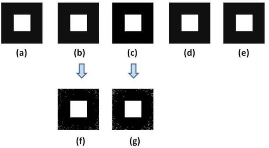
(47) 5. Experiments The color sensation output by the Retinex algorithms is an enhanced color image, where the chromatic dominant of the light and possible slight shadows are partially removed and the scene details are emphasized. In our comparative analysis of RSR, STRESS and QBRIX, we define a set of evaluation measures taking into account three visual properties of the color sensation, already used in previous works, e.g. [20] [9]: brightness, contrast, chromatic dynamic range. The analysis of these quantities allo w to evaluate the image enhancement produced by the algorithms o f the Retinex family . We remark that here we do not consider any pre- or post-filtering calibration of the input and output images, which is usually required by other tasks, e.g. for modeling the human vision system [21]. The proposed comparison is performed on the public dataset YACCD [19] that is composed by 168 pictures displaying seven ob jects portrayed against two textured backgrounds and under seven illuminants with and without shadows (see Fig. 3 for an example). The tests have been also performed on a simple image , named Test16.255, displaying a bright square (with uniform RGB color (255, 255, 255)) over a dark background (with uniform RGB color (16, 16, 16)). Due to its simple structure (see Fig. 4(a)), Test16.255 is commonly employed to visualize the filtering effects of spatial color algorithms.. Fig. 3 - An ex ample from YACCD: (A) the same image has been captured under seven different illuminants; (B) for each illuminant, the object is display ed against tw o different backgrounds, w ith and w ithout shadow s.. 5.1. Evaluation Measures. Brightness - We evaluate the brightness variation between the input image and its color filtered version by comparing their brightness mean values. Precisely, the mean image brightness is defined as (5.1). 47.