HAL Id: hal-03230043
https://hal.archives-ouvertes.fr/hal-03230043
Submitted on 19 May 2021
HAL is a multi-disciplinary open access archive for the deposit and dissemination of sci-entific research documents, whether they are pub-lished or not. The documents may come from teaching and research institutions in France or abroad, or from public or private research centers.
L’archive ouverte pluridisciplinaire HAL, est destinée au dépôt et à la diffusion de documents scientifiques de niveau recherche, publiés ou non, émanant des établissements d’enseignement et de recherche français ou étrangers, des laboratoires publics ou privés.
Euro-Atlantic planetary wave-breaking
Gabriele Messori, Paolo Davini, M. Carmen Alvarez-Castro, Francesco
Pausata, Pascal Yiou, Rodrigo Caballero
To cite this version:
Gabriele Messori, Paolo Davini, M. Carmen Alvarez-Castro, Francesco Pausata, Pascal Yiou, et al.. On the low-frequency variability of wintertime Euro-Atlantic planetary wave-breaking. Climate Dynamics, Springer Verlag, 2019, 52 (3-4), pp.2431-2450. �10.1007/s00382-018-4373-2�. �hal-03230043�
https://doi.org/10.1007/s00382-018-4373-2
On the low-frequency variability of wintertime Euro-Atlantic planetary
wave-breaking
Gabriele Messori1 · Paolo Davini3,4 · M. Carmen Alvarez‑Castro2,5 · Francesco S. R. Pausata1,6 · Pascal Yiou2 · Rodrigo Caballero1
Received: 6 August 2017 / Accepted: 15 May 2018 / Published online: 31 July 2018 © The Author(s) 2018
Abstract
Planetary wave-breaking can lead to large-scale atmospheric circulation anomalies and favour high-impact weather occur-rences. For example, the simultaneous occurrence of anti-cyclonic wave-breaking to the south of the North Atlantic jet and cyclonic wave-breaking to the north, here termed double wave-breaking, has been linked to heightened frequencies of explosive cyclones in the Atlantic basin and destructive windstorms over Western and Continental Europe. The present study analyses the long-term temporal variability of wintertime cyclonic and anti-cyclonic wave-breaking, and the resulting double wave-breaking, in the North Atlantic. We use reanalysis data, proxy reconstructions of the North Atlantic Oscilla-tion (NAO) and a 1000-year coupled global climate model equilibrium simulaOscilla-tion under constant pre-industrial forcing. The wave-breaking wavelet spectra highlight a significant ultra-centennial variability in double wave-breaking frequency, which is largely mirrored in the variability of the NAO. However, we note that the NAO wavelet spectra in the different datasets display significant discrepancies. The low-frequency wave-breaking variability is reflected in long-term anomalies of the large-scale atmospheric circulation in the Euro-Atlantic sector. The 100-year periods with the most and least double wave-breaking occurrences display significant and opposite anomalies in both upper and lower-level wind, as well as in the frequency of extreme temperature events and in the magnitude of wind destructiveness over Europe. The latter broadly resembles the wind destructiveness anomalies associated with individual double wave-breaking instances in reanalysis data. The existence of low-frequency variability in an atmospheric pattern related to high-impact weather events has important implications for the study and interpretation of climate change projections and of possible future NAO changes.
Keywords Planetary wave-breaking · Low-frequency variability · Windstorms · Millennium · North Atlantic · NAO
1 Introduction
Planetary wave-breaking (PWB) is commonly defined as the large-scale, irreversible overturning of potential vorti-city (PV) contours near the tropopause level (Hoskins et al. 1985).1 This process is associated with large-amplitude
atmospheric waves and its effects extend throughout the troposphere. Specific wave-breaking patterns therefore leave a clear signature in the large-scale atmospheric flow at all
levels from the surface to the tropopause (e.g. Riviere and Orlanski 2007; Strong and Magnusdottir 2008).
Depending on the direction of the overturning, PWB can be divided into cyclonic (CWB) and anticyclonic (AWB) epi-sodes. AWB over the Eastern Pacific and the North Atlantic has been identified as one of the dynamical triggers for the positive phase of the North Atlantic Oscillation (NAO; Bene-dict et al. 2004; Franzke et al. 2004), while CWB in the North Atlantic has been linked to the negative phase of the NAO and high-latitude atmospheric blocking (Woollings et al. 2008). On longer timescales, periods with more frequent wave-breaking (and/or blocking) over Greenland and Western Europe have been associated with weaker ocean–atmosphere heat fluxes and the warm phase of the Atlantic Multidec-adal Variability (AMV; Häkkinen et al. 2011; Rimbu et al.
Electronic supplementary material The online version of this article (https ://doi.org/10.1007/s0038 2-018-4373-2) contains supplementary material, which is available to authorized users. * Gabriele Messori
gabriele.messori@misu.su.se
Extended author information available on the last page of the article
1 Although PWB can occur at various levels in the atmosphere, the largest direct impact in the troposphere is usually seen as a result of PWB near the tropopause.
2014)—a low-frequency alternation of warmer and colder than usual sea-surface temperatures in the North Atlantic. The AMV, in turn, has been linked to changes in the occur-rence of positive and negative NAO phases (e.g. Peings and Magnusdottir 2014; Omrani et al. 2014; Davini et al. 2015), with a warm AMV phase favouring a negative NAO.
In the case of quasi-stationary waves, the signature of PWB can persistently affect specific domains, leading to large regional anomalies. Indeed, a number of recent studies have associated specific boreal winter wave-breaking patterns in the North Atlantic region with extreme weather occur-rences over the European continent. Hanley and Caballero (2012) analysed a set of historical windstorms over Europe, and found that the vast majority were preceded by the simul-taneous occurrence of anticyclonic wave-breaking to the south of the North Atlantic jet and cyclonic wave-breaking to the north, which they termed double wave-breaking (DWB). A similar wave-breaking pattern was later linked to particu-larly intense explosive cyclones (Gómara et al. 2014) and to cyclone clustering in the Euro-Atlantic sector (Pinto et al. 2014). Finally, Messori and Caballero (2015) showed that there is a robust statistical link between DWB in the eastern part of the North Atlantic basin and increased wind destruc-tiveness over continental Europe, although there is not a one-to-one correspondence between the two. Indeed, the authors found that eastern DWB leads to an almost doubling of the frequency of destructive windstorms over Western–Conti-nental Europe, but is neither a necessary nor a sufficient con-dition for the windstorms to occur (Messori and Caballero 2015; see also: Gómara et al. 2014; Priestley et al. 2017).
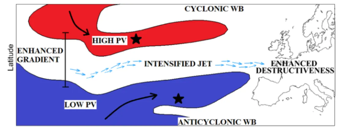
The DWB-windstorms link is mediated by the impact the former has on the large-scale atmospheric circulation. A cyclonic (anticyclonic) wave-breaking event leads to positive (negative) PV anomalies to the south (north) of the breaking latitude; when CWB occurs to the north of an AWB (in the Northern Hemisphere) the result is therefore to strengthen the meridional PV gradient. A stronger meridional PV gradient in turn implies a stronger westerly flow (Hoskins et al. 1985), meaning that DWB over Euro-Atlantic region is associated
with an intensified, more zonally-oriented Atlantic jet. The stronger jet favours the intensification of storms, while the enhanced zonality directs them towards Europe, thus favour-ing destructive winds over the continent (Messori and Cabal-lero 2015, Messori et al. 2016). This process chain is sum-marised in Fig. 1.
DWB over the North Atlantic is therefore robustly linked to societally and economically relevant wintertime extreme weather occurrences. In this perspective, it is important to identify whether this pattern displays any significant low-frequency natural variability and, if so, what the implica-tions for the large-scale atmospheric circulation and extreme weather episodes might be. This will also provide a bench-mark for evaluating the significance of changes in extreme weather occurrences found in climate-change simulations. While there is a literature looking at past trends and expected future changes in PWB and their interaction with the mid-latitude jet (e.g. Hood et al. 1999; Barnes and Hartmann 2012; Garfinkel and Waugh 2014), comparatively little attention has been devoted to the DWB’s temporal variabil-ity, especially on long (> decadal) time scales. Woollings et al. (2015), have recently related the multi-decadal vari-ability of the NAO to changes in the frequency of PWB on both sides of the jet. However, to the best of our knowledge there is no comparable study with an explicit focus on DWB and its footprint on the mean atmospheric state in the Euro-Atlantic region and on high-impact weather occurrences.
In the present paper, we aim to address this knowledge gap by detailing the low-frequency temporal variability of AWB, CWB and DWB statistics in the North Atlantic. In order to provide a comprehensive overview of this vari-ability, we use reanalysis data, proxy reconstructions of the NAO and a 1000-year Global Climate Model equilibrium simulation under constant pre-industrial (PI) forcing. The analysis encompasses both the wave-breaking variability itself and the associated atmospheric circulation and surface anomalies. The study is organised as follows: after describ-ing the datasets and methodology (Sect. 2), we discuss the variability of PWB from interannual to centennial timescales
Fig. 1 Schematic illustrating the impact of DWB on the large-scale flow. The thin black lines show idealised PV contours. The simultaneous AWB and CWB result in a strengthened meridional PV gradient, which leads to an intensified zonal jet. This, in turn, favours enhanced wind destructiveness down-stream of the DWB (Messori and Caballero 2015)
(Sect. 3). We then analyse the impact of the DWB’s low-frequency variability on the large-scale atmospheric dynam-ics and on destructive windstorms over Europe (Sect. 4). Section 5 compares the results of the millennial simulation to reanalysis and proxy datasets, while Sect. 6 concludes the study by summarising our main findings and discussing their implications for extreme event occurrences over the European continent.
2 Data and methodology
2.1 Model and reanalysis data
This study is based on 6-h data from a 1000-year PI control simulation of the Max–Planck-Institute Earth System Model (MPI–ESM). The MPI–ESM consists of the ECHAM6 atmospheric model (Stevens et al. 2013), the MPIOM ocean model (Jungclaus et al. 2013) and the JSBACH (Reick et al. 2013; Schneck et al. 2013) and HAMOCC5 (Ilyina et al. 2013) subsystem models for land/vegetation and marine bio-geochemistry, respectively. Here we use the MPI–ESM–P version, which has a T63 horizontal resolution (~ 1.9°), 47 vertical levels in the atmosphere from the surface to 0.01 hPa, and uses prescribed vegetation (Giorgetta et al. 2013).
The PI simulation uses a constant forcing and 1850 orbital parameters. Forcing components which depend on the solar cycle, such as solar irradiance and ozone concentration, are averaged over 11 year periods centred at, or close to, 1850. Only tropospheric natural aerosols are taken into account, while volcanic aerosols are excluded altogether. For further details on the model and experimental setup the reader is referred to Giorgetta et al. (2013).
Part of the analysis is also based on the NCEP/NCAR reanalysis (Kalnay et al. 1996), over the 1950–2010 period. The data has a horizontal resolution of 2.5°. For the PWB analysis, we have opted not to use century-long products such as the twentieth Century Reanalysis (Compo et al. 2011) or ECMWF’s ERA-20C (Poli et al. 2016) because a comparison of these datasets with some limited observations from the early twentieth century suggests that the biases in mid and upper-level tropospheric flows in the North Atlan-tic sector are large (SAtlan-tickler et al. 2015). While it is hard to determine whether the PWB spectra are affected by this or not, it is certainly a feature that deserves further investiga-tion, beyond the scope of the present paper. For reference, we show the ERA-20C and the twentieth Century Reanalysis AWB and CWB wavelet spectra in Fig. S1.
All the analysis is based on the canonical boreal winter period (December-February, DJF). In Sect. 4, anomalies are defined as deviations from the 1000-year model DJF clima-tology. Statistical significance is assessed using Monte Carlo
random sampling with 1000 iterations. First, distributions of outcomes based on random sets of winter seasons are created. Next, one-sided 95% confidence bounds are obtained directly from the percentiles of these distributions.
2.2 Climate indices
The AMV is a mode of natural variability of the North Atlan-tic Ocean (Schlesinger and Ramankutty 1994). Here we com-pute the AMV index following Trenberth and Shea (2006). First we compute yearly anomalies of area-averaged SST over the North Atlantic (0–60° N, 0–80° W). We then subtract the global (60° S–60° N) mean SST and apply a 10-year running mean smoothing.
The North Atlantic Oscillation Index (NAOI) is defined as the standardised principal component of the first EOF of the monthly mean 500 hPa geopotential height (Z500) over the North Atlantic sector (90° W–40° E, 20°–85° N) during DJF. The NAO phase is positive when a low-pressure anomaly is present over Iceland and a high-pressure anomaly is found over the Azores.
To test the behaviour of the modelled NAOI we further make use of two proxy reconstructions. The first (Luterbacher et al. 2001) combines long-term instrumental and documen-tary proxy evidence to extend and improve previous NAO estimates, and provides a monthly NAO index back to 1659 and a seasonal NAO index back to 1500. In our analysis, we take the DJF mean from the monthly dataset and analyse the full wintertime NAO series from 1500 to 1995. The second reconstruction (Ortega et al. 2015) provides a yearly NAO index for the past millennium (1049–1969), determined from a sub-selection of 48 annually-resolved paleoclimate archives.
2.3 Wave‑breaking algorithm
In order to objectively detect PWB, we make use of the bidi-mensional Wave Breaking Index (WBI) developed by Davini et al. (2012). The index estimates the location and direction of rotation of the wave-breaking using reversals of the Z500 meridional gradient on data interpolated to a regular 2.5° × 2.5° grid (Tibaldi and Molteni 1990; Scherrer et al. 2006; Davini et al. 2012).
For every grid point with coordinates (λ0, φ0) we define:
GHGS(𝜆0, 𝜑0) = Z500(𝜆0, 𝜑0) − Z500(𝜆0, 𝜑s)
𝜑0− 𝜑s
GHGN(𝜆0, 𝜑0) =
Z500(𝜆0, 𝜑N) − Z500(𝜆0, 𝜑0) 𝜑N− 𝜑0
where φ0 ranges from 30° N to 75° N and λ0 ranges from
0° to 360°. φs = φ0 – 15°, φN = φ0 + 15°. An Instantaneous Blocking (IB) is identified if:
Once the grid points where the reversal is occurring are defined, we use the horizontal gradient of Z500 (measured 7.5° south of the reversal itself, in order to fully capture the wave-like structure) to assess whether these are associated with AWB or CWB. The WBI is then defined as:
where λW = λ0 – 7.5° and λE = λ0 + 7.5°. Thus, the WBI
dis-tinguishes between anticyclonic PWB events (Z500 decreas-ing eastward, WBI < 0) and cyclonic PWB events (Z500 increasing eastward, WBI > 0).
This approach, which is grounded in the geostrophic approximation of the method based on the horizontal stretching deformation introduced by Kunz et al. (2009), is similar to the one adopted by Masato et al. (2012). More importantly, it is consistent with the areas and frequen-cies of wave-breaking defined in the literature, including methods based on the reversal of the meridional potential GHGS(𝜆0, 𝜑0) > 0 GHGN(𝜆0, 𝜑0) <−10 m∕◦lat. WBI(𝜆0, 𝜑0) = Z500(𝜆W, 𝜑S+ 7.5◦) − Z500(𝜆 E, 𝜑S+ 7.5◦) 𝜆W− 𝜆E
temperature gradient on the 2-PVU surface (Tyrlis and Hoskins 2008; Strong and Magnusdottir 2008). Full details on the WBI and its derivation can be found in Davini et al. (2012).
We then use the output of the above algorithm to define DWB in the Euro-Atlantic sector (70°W–20° E, 30°–75° N). A DWB event occurs when an AWB is identified within the part of the target domain south of 45°N while a CWB simultaneously occurs north of 55°N. These domains are illustrated by the black boxes in Fig. 2a, b. We define sim-ultaneity as meaning that the two WB episodes are detected on the same day. The meridional thresholds are imposed to select AWB and CWB events occurring on the equatorward and poleward flanks of the climatological jet respectively, such that they correspond to the anomalous jet configura-tion discussed in Sect. 1. Messori and Caballero (2015) have shown that these fixed thresholds successfully capture the desired DWB events in both reanalysis data and the MPI-ESM model, notwithstanding the large variability in the jet’s meridional location. We also note that these two domains match the regions displaying the highest frequencies of Greenland CWB and southern North Atlantic AWB. When an AWB/CWB pair occurs outside the specified domains, it is ignored. We further require that the PWB pair forming the DWB be longitudinally aligned—namely that there is at least one longitude at which one gridbox in each domain is identi-fied as a PWB location. These criteria result in just over 9
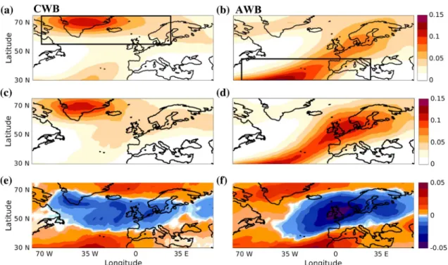
Fig. 2 Climatological frequency of CWB (a, c) and AWB (b, d) (breakings/day/gridbox) in a, b the MPI-ESM-P model and c, d the NCEP/NCAR reanalysis. e, f Display the model-reanalysis
differ-ences. The black boxes in a and b mark the domains used to define DWB. The data for NCEP/NCAR covers DJFs over the period 1950– 2010
DWB episodes per winter in the NCEP/NCAR reanalysis and just over 12 in the MPI-ESM data.
The results presented in the rest of the study are highly sensitive to the choice of restricting our CWB domain to the north of the climatological location of the jet and the AWB domain to its south. Indeed, if the domains are modified but still primarily capture wave-breaking pairs straddling the jet, the spectra discussed below show relatively minor changes. Radical changes are instead found if the domains are changed so as to include wave-breaking pairs occurring on the same flank of the jet (not shown). These, however, are very different from the dynamical interpretation of DWB we focus on here (see Fig. 1), and we do not address them in this study.
In a previous analysis based on ERA-Interim data, Mes-sori and Caballero (2015) have shown that DWB in the east-ern part of the North Atlantic basin was the most effective in driving a large-scale zonalisation and intensification of the jet stream, while DWB episodes occurring further west resulted in no intensification or even a weakening of the zonal flow over the jet exit region. In the MPI-ESM model, we instead find that DWB across the whole basin has a simi-lar impact on the simi-large-scale flow (see Fig. S2). This justi-fies the use of a broad Atlantic sector in defining DWB. We interpret this discrepancy as the result of both model biases in the large-scale circulation and the different PWB algo-rithm and DWB selection processes used here compared to previous studies.
2.4 Wavelet transforms
We use continuous wavelet transforms to provide a time-dependent picture of the spectral power of the PWB fre-quency time series. Wavelet transforms can be implemented using a variety of different wavelet classes; throughout our analysis we the Morlet wavelet—which is generally appro-priate for the analysis of geophysical timeseries—with wavenumber ω = 6, the smallest scale set at twice the sam-pling time (i.e. two seasons) and the spacing between dis-crete scales set at 0.25. In wavelet transforms, the wavelet scale does not necessarily correspond to the Fourier period, although an analytical relationship between the two can be computed and, for Morlet wavelets, the two are usually very close. In all the figures the spectra are plotted as a function of equivalent Fourier period as opposed to wavelet scale.
All the timeseries are detrended and normalised to have zero mean and unit standard deviation before applying the wavelet transform. The global wavelet spectrum is computed by integrating the spectral power at all timesteps in the data-set. We note that, in computing the global spectra, we only take into account values within the cone of influence, namely the region of the spectrum not influenced by edge effects. We further discuss plots of cross-spectral wavelet power,
coherence and phase. Cross-spectrum plots indicate regions of the time–frequency space where two signals display com-mon spectral power. Wavelet coherence can be interpreted as a local indicator of correlation in time–frequency space. Finally, wavelet phase illustrates the relative phase between the signals, again in time–frequency space. The phase angles are measured counter-clockwise. Right-pointing arrows correspond to a zero angle; upward or downward pointing arrows to signals in quadrature (90° and 270°, respectively) and left-pointing arrows (180°) to an out-of-phase relation-ship. We evaluate the statistical significance of the wavelet power spectra, global spectra and cross-spectra against the null hypothesis of an AR1 process with the lag-1 autocor-relations estimated from the timeseries analysed. We use a Chi-squared test, following Torrence and Compo (1998). The significance of the wavelet coherence is computed using Monte Carlo iterations to generate an ensemble of 1000 sur-rogate data set pairs with the same AR1 coefficients as the input datasets, following Grinsted et al. (2004). All figures display 95% confidence bounds.
For further details on the properties of the Morlet wave-let, on wavelet transforms in general and on how to com-pute spectral coherence and phase, the reader is referred to Goupillaud et al. (1984), Torrence and Compo (1998) and Grinsted et al. (2004). Links to the publicly available wavelet codes used in this analysis are provided in the acknowledgements.
3 Planetary wave‑breaking variability
3.1 Wave‑breaking climatology and spectra
During wintertime, AWB over the North Atlantic is typi-cally concentrated in the southern and eastern portions of the basin, while CWB primarily occurs further north. However, both PWB types can occur on either side of the jet stream. Figure 2 shows the PWB wintertime climatology for both the MPI-ESM model (Fig. 2a, b) and the NCEP/NCAR data (Fig. 2c, d). The MPI-ESM model successfully captures the geographical distribution of PWB events, although it dis-plays some biases in the frequency. Most CMIP5 models overestimate low-latitude blocking activity and underesti-mate the frequency of mid and high-latitude events (Anstey et al. 2013). A similar pattern emerges in terms of PWB. The model produces too many low-latitude AWBs, while too few AWB episodes occur over the British Isles and Northern and North-Eastern Europe. A positive bias is also seen at the northern edge of the domain (Fig. 2f). Biases in CWB are somewhat similar, although the region in which the model displays the strongest negative bias is shifted to the west, spanning from Greenland to Western–Continental Europe (Fig. 2e).
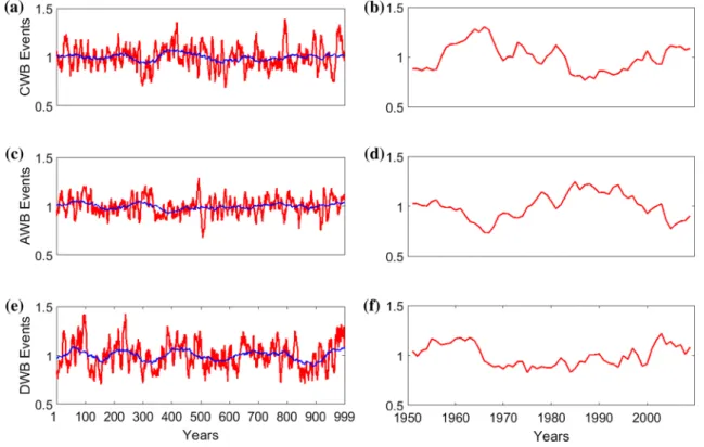
We next construct timeseries of the number of AWB and CWB events per season in the domains defined in Sect. 2.3. The normalised, smoothed timeseries are shown in Fig. 3 for both the MPI-ESM model and the NCEP/NCAR reanalysis. The reanalysis displays multi-annual to decadal variability in all three timeseries, with some indication of lower-frequency modulations (Fig. 3b, d, f). The model AWB and CWB data show a marked decadal to multi-decadal variability (Fig. 3a, c), while the DWB timeseries is dominated by lower fre-quency oscillations, which also emerge clearly in the 101-year running mean (blue line in Fig. 3e).
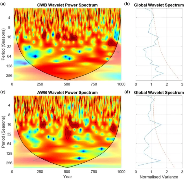
A number of these features are confirmed by a more rig-orous spectral analysis of the timeseries. The continuous wavelet spectra of the MPI-ESM model clearly show that both cyclonicities display heightened spectral power around 16-year periods throughout most of the simulation, although this is only locally significant (Fig. 4a, c). Consistently with this, both global spectra (Fig. 4b, d) display a significant spectral peak at 16 years. A secondary non-significant peak at ultra-centennial scales, close to the limit of the resolved periods, is also seen.
Both these peaks are captured by the cross-wavelet spec-trum (Fig. 5a), which displays significant common power at these periods. Furthermore, while the highest common power at ultra-centennial timescales is found in the first half of the simulation, there is a clear signal extending across
the cone of influence (see Sect. 2.4). The two timeseries are systematically in anti-phase around 16 years (Fig. 5b, arrows), and indeed in virtually all regions where coher-ence is significant (Fig. 5b, colours). The two exceptions are periods around 64 years and ultra-centennial scales, where phase angles of 135° or less (i.e. pointing in a north-westerly or north-north-westerly direction) are seen. However, only the second of these two regions shows any significant cross-spectral power. We note that if two phenomena are physi-cally linked at a given timescale, they can be expected to show a phase-locked behaviour (e.g. Grinsted et al. 2004). The systematic phase relationship between the AWB and CWB signals is reassuring in this respect.
The DWB spectrum displays extensive areas of signifi-cant power (Fig. 6a) and a significant global wavelet peak (Fig. 6b) at ultra-centennial scales, again at the limit of the cone of influence. Since DWB requires the simultaneous occurrence of an AWB and a CWB, the DWB timeseries is unlikely to display a strong variability at frequencies where the two are in anti-phase. This will instead be seen at fre-quencies where the two cyclonicities display high common power, high coherence and a more favourable phase relation-ship, as indeed we find here.
An initial analysis of the spectrum of wintertime PWB frequencies over the North Atlantic therefore points to the existence of a multi-decadal variability in AWB and CWB
Fig. 3 Normalised, detrended DJF count of CWB (a, b), AWB (c, d)
and DWB (e, f) episodes in the domains specified in Sect. 2.3, in a, c,
e the MPI-ESM-P model and b, d, f the NCEP/NCAR reanalysis. The
red lines show data filtered with an 11-season running mean, while the blue lines correspond to a 101-year running mean. The data for NCEP/NCAR covers DJFs over the period 1950–2010
and a very low-frequency variability in DWB. The lat-ter confirms the visual appraisal of the timeseries shown in Fig. 3e. As already remarked, the low-frequency DWB spectral peak lies at the edge of the cone of influence and should therefore be interpreted with care. To test that it is indeed a physically relevant feature we perform an analysis of the large-scale atmospheric anomalies during centuries with high and low DWB frequencies. We find that the low-frequency DWB variability has a well-defined footprint on the large-scale dynamics, as described in detail in Sect. 4.1.
3.2 Links to large‑scale modes of variability
We next verify whether the above spectral features can be related to known modes of climate variability, such as the
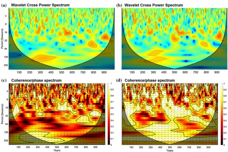
NAO. As discussed in the introduction, there are extensively documented links between PWB and the NAO; the NAO is further known to display variability on a broad range of timescales (e.g. Woollings et al. 2015 and references therein). The NAOI’s global wavelet spectrum displays three prominent peaks: one at interannual timescales, one centred on a 16-year period and one at ultra-centennial scales, with the middle peak having the highest significance (Fig. 6d). The latter peaks roughly match those seen in the AWB and CWB spectra. Even though none of the low-frequency spec-tral peaks in the AWB, CWB and NAO spectra are globally significant, the cross-wavelet spectra of the NAO and the two PWB signals show locally significant common power at those periods (Fig. 7a, b). The phase spectra (Fig. 7c, d) highlight a systematic in-phase (anti-phase) relationship
Fig. 4 The continuous (a, c) and global (b, d) wavelet spectra of CWB (a, b) and AWB (c, d) in the MPI-ESM-P model. The thin black contours in a, c designate statistically significant regions. The
thick black contours mark the cone of influence. Red (blue) colors correspond to high (low) spectral power. The dashed red lines in b, d indicate the respective 95% confidence levels
between the NAO and AWB (CWB) frequency. This is con-sistent with the synoptic interpretation of the NAO as being associated with anti-cyclonic (cyclonic) breaking during its positive (negative) phase (e.g. Benedict et al. 2004; Franzke et al. 2004; Strong and Magnusdottir 2008).
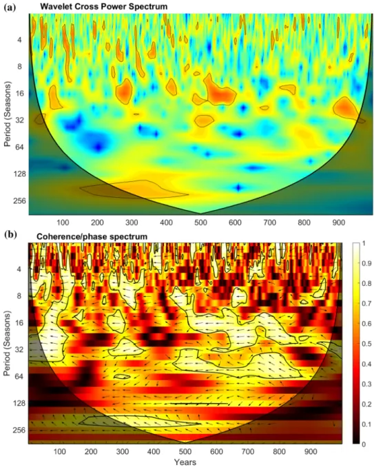
The NAO-DWB cross-spectra (Fig. 8) further reveal that there is significant common power (Fig. 8a) and a high coherence (Fig. 8b) between the NAO and the DWB at ultra-centennial timescales, although this is again primarily seen in the first half of the model simulation. The large phase angles seen in Figs. 7c and 8b suggest that, at these very long periods, DWB favours the negative NAO phase (although the two are not exactly in anti-phase) and heightened CWB occurrences in the northern part of the North Atlantic basin. The low ultra-centennial coherence between the NAO and
DWB occurrence in the later part of the model simulation can be ascribed to the decreased coherence between AWB and CWB counts over the same time period and timescale. We specifically note that the lowest coherence values in both the AWB/CWB and DWB/NAO coherence/phase spectra fall in the periods between ~ 100 and 200 years, with the longest periods displaying instead higher coherence values throughout the model simulation (cf. Figs. 5b, 8b). We there-fore conclude that the DWB–NAO link is modulated by the co-variability of AWB and CWB, which are the dynamical features having a direct bearing on the NAO’s phase.
A second variability mode potentially associated with the low-frequency variability in PWB occurrences is the AMV (see Sects. 1, 2.2). As expected, the AMV displays high spectral power at multi-decadal timescales, but does
Fig. 5 a Wavelet AWB/CWB
cross-spectrum in the MPI-ESM-P model. Red (blue) colors correspond to high (low) common power. b AWB/CWB coherence (colours) and phase (arrows). The arrows’ direc-tion indicates the phase angle. Right-pointing arrows cor-respond to a zero angle; upward or downward pointing arrows to signals in quadrature and left-pointing arrows to an out-of-phase relationship. Note that phase is only shown in regions where the coherence exceeds 0.5. The thick black contours mark the cone of influence. The thin black contours designate statistically significant regions
not display a significant signal at the longest periods resolved by the wavelet spectrum. We further find a rela-tively low coherence with the AWB and CWB frequencies at 16 year periods, albeit with locally significant common power. These figures are not shown. In the model simula-tion, the AMV therefore has a relatively weak link with the low-frequency variability of PWB over the North Atlantic.
A possible interpretation of the 16-year PWB periodic-ity is given by the work of Manzini et al. (2012). Using a similar model setup (which included the atmospheric model ECHAM5 with 95 vertical levels from the sur-face to 0.01 hPa), they found a 20-year periodicity in the stratospheric polar vortex. This could potentially affect the lower tropospheric North Atlantic PWB driving a perio-dicity similar to that observed in the MPI-ESM-P simu-lation; however, a study of the stratosphere-troposphere
coupling in the model is beyond the scope of the present study.
4 Atmospheric flow anomalies associated
with DWB variability
4.1 Large‑scale anomalies in the Euro‑Atlantic sector
The above spectral analysis has highlighted a significant var-iability in DWB occurrence over the North Atlantic at ultra-centennial timescales. Here, we verify whether this variabil-ity has a strong footprint on the large-scale atmospheric flow. We begin by selecting the 100 years with the most (DWB+) and least (DWB–) DWB occurrences. The DWB+ period
Fig. 6 The continuous (a) and global (b) wavelet spectra of DWB in the MPI–ESM–P model. All markings are as in Fig. 4. c, d Same as (a, b) but for the NAOI
corresponds to a statistically significant increase in the total number of episodes by roughly 9% relative to the climatol-ogy, while the DWB-period corresponds to a statistically significant decrease of over 11%. We choose 100 years as an indicative length of a period of high/low DWB occurrence associated with the ultra-centennial variability.
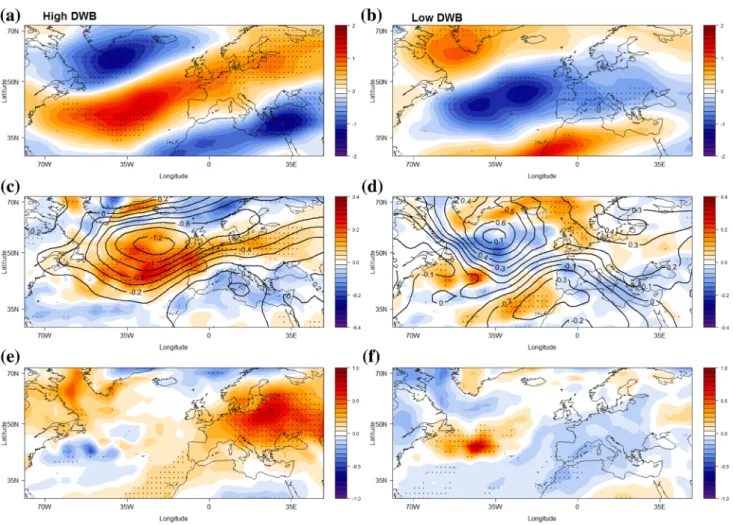
The 300 hPa wind anomalies for the DWB+ period (Fig. 9a) display a tripolar anomaly pattern, corresponding to an intensified mid-latitude jet across the North Atlantic basin. This is consistent with the dynamical interpretation provided in Fig. 1, whereby the DWB results in a sharp-ened, intensified zonal flow. This pattern is mirrored by the 10-m wind (Fig. 9c, colours), indicating a predominantly barotropic structure of the anomalies. We further note that the 10-m wind shows a band of positive anomalies spanning northern continental Europe, associated with a negative SLP pole to the west of the British Isles (Fig. 9c, contours). This flow corresponds to the anomalous advection of moist oce-anic air masses across the continent, leading to warm tem-perature anomalies across most of Eastern Europe (Fig. 9e). The DWB− period displays roughly opposite anomalies. The upper-level westerly flow at the climatological jet lati-tude is significantly weakened, while positive anomalies are
found on the southern edge of the Mediterranean basin and across the northern North Atlantic and Scandinavian penin-sula (Fig. 9b). A similar picture is seen for the 10-m wind, albeit with a less well-defined meridional anomaly tripole. The flow over much of Iberia and France is now weakened relative to the climatological values. This structure is associ-ated with a longitudinally elongassoci-ated high-pressure anomaly stretching from Scandinavia to Greenland and a low pres-sure anomaly centred over southern Iberia and the Canary Islands (Fig. 9d). The temperature footprint over land is rela-tively weak and only locally significant, with small nega-tive anomalies spanning most of Western Europe and the Mediterranean basin (Fig. 9f).
The SLP anomaly patterns of the two periods project weakly on the NAO. Both display meridional dipoles, but neither is aligned with the canonical NAO centres of action over the Azores and Iceland. We further note that the SLP anomalies associated with DWB– are approximately half the magnitude of the DWB+ ones. The low-frequency co-variability of DWB and the NAO is associated with large phase angles (and thus a negative projection of DWB on the NAO, Fig. 8b) but this does not emerge clearly in Fig. 9c, d.
Fig. 7 Wavelet CWB/NAO (a) and AWB/NAO (b) cross-spectra in the MPI-ESM-P model. CWB/NAO (c) and AWB/NAO (d) coherence (col-ours) and phase (arrows). All markings are as in Fig. 5
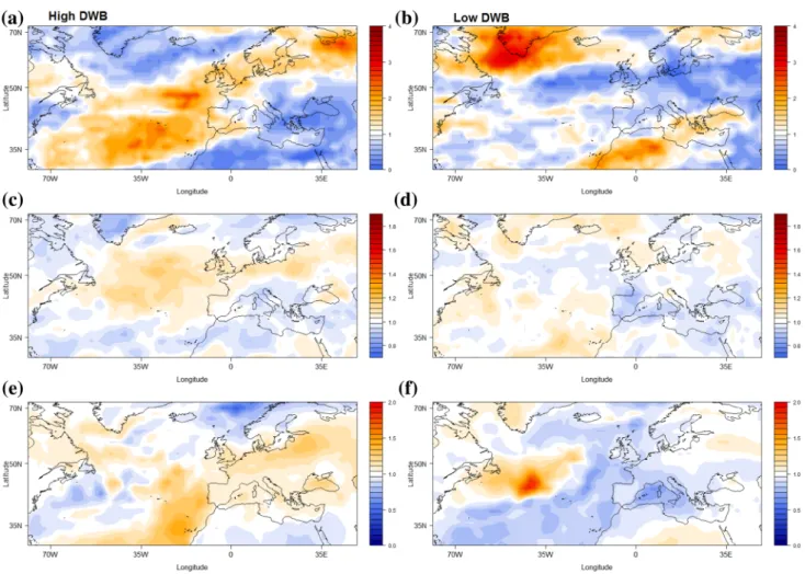
We next investigate whether the above anomalies in the large-scale atmospheric flow and temperature patterns correspond to changes in the frequency of extreme events (Fig. 10). These are defined as values exceeding the 95th percentile of the local distribution of each variable for the full 1000 DJFs in the model simulation. The analysis was repeated for different definitions of extremes (ranging from the 90th to the 99th percentile) and qualitatively similar results were obtained. For reference, we show the results for the 98th percentile in Figure S3. We assess the changes in the probability of extreme event occurrences by building two new distributions, one for the DWB+ period and one for the DWB– period. We then compute the ratio between the frac-tion of days in each of the two distribufrac-tions at each gridbox
that exceed the original 95th percentile threshold and the fraction of days that exceed the 95th percentile of the respec-tive climatological distributions (i.e. 5% of days). A value of 1 indicates that the frequency of the extremes in the selected period is the same as in the climatology; values below 1 indicated a decreased extreme event frequency, while val-ues above 1 indicate an increased frequency. For example, for our chosen threshold a value of 2 would imply that 10% of the days in the selected period qualify as extremes. The upper-level wind for the DWB+ period displays a band of heightened extreme event frequency roughly matching the area of positive wind speed anomalies, with local increases exceeding 200% (cf. Figs. 9a, 10a). The same is found for the 10-m wind, which displays frequency increases ranging
Fig. 8 a Wavelet DWB/NAO
cross-spectrum in the MPI-ESM-P model. b DWB/NAO coherence (colours) and phase (arrows). All markings are as in Fig. 5
between 15 and 40% across much of northern Continental Europe (Fig. 10c). This feature will be discussed further below in the context of destructive windstorms. The 2-m temperature extremes also match the previously shown anomaly pattern, with almost 1.5 times the climatological frequency of extremes in the Baltic States, which correspond to the region displaying the largest absolute anomalies (cf. Figs. 9e, 10e).
The DWB– period also shows frequency changes which match the large-scale anomaly patterns. The extreme upper-level wind episodes along the climatological jet track are roughly halved, and locally almost absent (Fig. 10b). Simi-larly, 10-m wind extremes show a decrease in frequency across most of Western and Continental Europe (Fig. 10d). The temperature extremes show similarly marked changes, with sharp decreases across most of Western and Continen-tal Europe (Fig. 10f).
Low-frequency changes in DWB occurrence therefore lead to very large changes in the occurrence of extreme events across the continent. Interestingly, the changes in
extreme event frequency during the two selected periods relative to the climatology are much larger than those in DWB frequency. The correspondence between DWB epi-sodes and extremes therefore appears to change between the two periods analysed, with the caveat that other low-frequency drivers not considered here might be at play. Coupled with the significant anomalies in the large-scale mean fields discussed above, this suggests that the changes in DWB frequency might be associated with a shift in the long-term dynamical regime of the atmosphere, in turn lead-ing to different extreme event statistics.
4.2 Destructive European windstorms
The largest increases in 10-m wind extremes over land are mostly confined to a region encompassing France, Germany, Benelux, Denmark and Poland (Fig. 10c). This is a densely-populated, heavily industrialised area which incurred a high level of insured losses from destructive windstorms in the 1990s. Since infrastructure is typically adapted to the local
Fig. 9 a, b 300 hPa wind speed anomalies (m s−1); c, d 10-m wind speed (m s−1, colours) and SLP (hPa, contours) anomalies; d, e 2-m tempera-ture anomalies (K) during (a, c, e) high DWB and (b, d, f) low DWB periods (see text). Stipling indicates statistically significant anomalies
conditions, we define wind destructiveness in terms of the significant power dissipation above a local threshold. This is chosen as the climatological 98th percentile wind speed (v98) at each point. For data points where v > v98, the wind
destructiveness is then given by:
Here, v is the daily maximum of the 6-hourly 10-m wind. The destructiveness at all other points is set to zero. This algorithm was originally proposed by Klawa and Ulbrich (2003); we select it here because it was developed using station wind data and annual insurance losses due to wind-storms in Germany, and is thus directly relevant to the social and economic damage caused by intense surface winds over Western Europe. We focus on land points, which is where the bulk of the damage to infrastructure and human activities typically occurs. As a caveat we note that since coastal grid points usually include a mix of land and ocean—where the wind speeds are much higher than on land—our method may underestimate destructiveness in coastal regions.
destr. =(v/v 98− 1
)3
The DWB+ period is characterized by a band of increased destructiveness relative to the climatology, stretching from the Iberian Peninsula across the continent to Eastern Europe (Fig. 11a, contours); lowered values are instead seen over northern Scandinavia and South-Eastern Europe, closely matching the region of decreased low-level wind speed extremes (Fig. 9c). The DWB– period (Fig. 11b), on the contrary, displays predominantly negative anomalies across Continental and Western Europe, with heightened values over Northern Scandinavia and the Eastern Mediterranean, roughly matching the regions of decreased destructiveness in the DWB+ period. The correspondence with the changes in low-level extreme wind episodes is weaker than for the DWB+ period (cf. Fig. 9d), suggesting that the increased destructive-ness in these regions may be linked to a small number of very intense episodes. Finally, the difference between the DWB+ and DWB– periods again highlights the increased windstorm destructiveness across Western and Continental Europe associ-ated with more frequent DWB occurrences (Fig. 11c).
Fig. 10 Relative changes in the frequency of (a, b) 300 hPa wind speed; c, d 10–m wind speed and (e, f) 2–m temperature extremes for the (a, c,
5 Comparison with reanalysis and proxy
data
Our analysis of PWB frequency over the North Atlantic in a long PI-control simulation of the MPI–ESM–P model has highlighted a significant variability at multi-decadal and longer timescales. A geographically comprehensive record of atmospheric observations is largely limited to the last five to six decades, implying that it is hard to verify to what extent these slow modes exist in the real world. While century-long reanalysis products are available, it is unclear whether they reproduce a realistic variability in PWB frequency during the earlier part of their record (see Sect. 2.1). Nonetheless, datasets like the NCEP/NCAR reanalysis allow us to investigate PWB frequency spectra up to near-vicennial timescales. We can therefore verify the degree to which the higher frequency features found
in the modelled spectra for AWB and CWB match the reanalysis data.
We begin with the global wavelet spectra of the AWB and CWB frequencies, defined exactly as in the model (Fig. 12a, b, respectively). Similarly to the model, both spectra display significant peaks, high coherence and an anti-phase relation-ship across most of the frequency-time space (not shown). However, while in the model the most prominent peaks for both cyclonicities were found at periods of 16 years, the NCEP/NCAR reanalysis is dominated by an 8-year cycle, with the AWB displaying a secondary peak around 5 years.
The 8-year PWB peak is closely mirrored by the NAO spectrum (Fig. 12c). This is in good agreement with a num-ber of past studies that have found peaks in the NAOI’s power spectrum at 6–10 year timescales (e.g. Hurrell and van Loon 1997; Pozo-Vazquez et al. 2001). A cross-spec-tral analysis shows that the NAO and the PWB signals have
Fig. 11 Normalised wind destructiveness (colours) and wind destruc-tiveness anomalies (contours) for the (a) high DWB and (b) low DWB periods. c Normalised wind destructiveness difference between the two periods. Normalisation of (a) and (b) is performed relative to
the peak wind destructiveness value in the high DWB period. Nor-malisation of (c) is performed relative to peak difference between the two periods. Stipling in (c) indicates statistically significant differ-ences
high common power (Fig. 13a, b), high coherence and a locked phase relationship at this timescale (Fig. 13c, d). As expected, AWB is systematically in-phase with the NAO, while the opposite is seen for CWB. While there is a factor of two difference in the period of the spectral peaks seen in the model and reanalysis, the interaction of the PWB and the NAO is qualitatively consistent across both datasets. Furthermore, studies using long observational records have highlighted that the NAO’s spectral power is highly discon-tinuous in time (e.g. Appenzeller et al. 1998; Pozo-Vazquez et al. 2001). Appenzeller et al. (1998) analysed a 350-year NAOI timeseries based on ice-core data, and found several periods with significant spectral power beyond 10 years and long periods with very little power at 8 years. Moreover, we note that the NAO spectrum in the 20CR and ERA-20C reanalyses displays a non-significant peak at 8 years and a second peak of similar magnitude at around 20 years (not shown).
An analysis of the two proxy datasets described in Sect. 2.2 also highlights a weak and discontinuous variabil-ity at interannual to decadal timescales (Fig. 12d, e). The only significant peaks are at multi-decadal to ultra-centen-nial scales, with the latter matching relatively closely the 130–150 year peak seen in the model NAO (Fig. 6d). An obvious caveat is that for the Luterbacher et al. (2001) index,
this is at the very edge of the cone of influence—namely of the frequencies that can be resolved without encounter-ing edge effects. We further observe that the double peak seen in the Ortega et al. (2015) index matches very closely those seen in the model’s DWB spectrum. The differences between the spectra of the two indices do not depend on the different temporal resolutions and time periods covered (see Sect. 2.2): repeating the analysis over the common time period and for yearly NAO values does not result in more similar spectra (not shown).
The above results therefore need to be interpreted with care for a number of reasons. Firstly, due to the large uncertainties present in the reconstructions of the NAO index for the pre-instrumental period (e.g. Luterbacher et al. 2001; Pinto and Raible 2012), compounded by the difficulty of dealing with a teleconnection pattern that may not be stationary in time (Schmutz et al. 2000; Ortega et al. 2015). Additionally, the fact that the Ortega et al. (2015) reconstruction provides annual data dilutes the signal of the winter NAO with information from the other seasons. Finally, we highlight that the MPI-ESM’s NAO spectrum (Fig. 6c) does present periods where there is significant spectral power in the 6–10 year band, and that the spectral variability at these scales might be affected by the constant 1850 radiative forcing used in the model
Fig. 12 The global wavelet spectra of AWB (a), and CWB (b) in the NCEP/NCAR reanalysis. The global wavelet spectra of the NAO index in the NCEP/NCAR renalysis (c) and the Luterbacher et al.
(2001) (d) and Ortega et al. (2015) (e) reconstructions. The dashed red lines indicate the respective 95% confidence levels
simulation analysed here. While it is difficult to come to an unambiguous conclusion on the variability of the NAO spectrum from the available data, the most relevant points are that:
1. Both the model and reanalysis display the same cross-spectral relation between the NAO and PWB over the North Atlantic. This suggests that the model simulation successfully captures the underlying dynamical link between these two features. We emphasise that this is far from trivial, since many CMIP5 models are unable to replicate this linkage (Davini and Cagnazzo 2014). 2. The low-frequency variability in the model is partially
supported by two long-term reconstructions of the NAO index, with the caveat that these reconstructions have large uncertainties and show important discrepancies. Moreover, the DWB spectrum in the reanalysis has no significant spectral peaks over the resolved timescale range, although there is a band of heightened spectral power at around 12 years (not shown). This is consistent
with the model’s DWB spectrum, which does not display any interannual or decadal peaks either.
6 Discussion and conclusions
In the present study, we highlight the existence of a sig-nificant multi-decadal to ultra-centennial variability in wintertime planetary wave-breaking frequency using data from a millennium-long simulation of the MPI-ESM-P model. These low frequency variability modes are partly mirrored in the variability of the winter NAO. It is of particular interest that the frequency of double wave-breaking—namely the co-occurrence of a cyclonic and an anti-cyclonic overturning—shows a significant peak at ultra-centennial periods. At these periods, DWB has a pre-dominantly anti-phase relationship with the NAO as has CWB, suggesting that this variability is primarily associ-ated with heightened CWB occurrences in the northern part of the North Atlantic basin.
DWB has previously been linked to an intensifica-tion and zonalisaintensifica-tion of the North Atlantic jet stream, a
Fig. 13 Wavelet CWB/NAO (a) and AWB/NAO (b) cross-spectra in the NCEP/NCAR reanalysis. CWB/NAO (c) and AWB/NAO (d) coherence (colours) and phase (arrows). All markings are as in Fig. 5
strengthening of the storm track activity and a heightened frequency of extreme weather occurrences over the Euro-pean continent (Hanley and Caballero 2012; Gómara et al. 2014; Pinto et al. 2014; Priestley et al. 2017). The above large-scale features are better indicators of destructive windstorm episodes than a purely NAO-based approach, thus motivating the interest in DWB activity (Messori and Caballero 2015; Messori et al. 2016). Here, we find that DWB is associated with significant large-scale flow anom-alies even on centennial and longer timescales. In particu-lar, the 100-year periods with the most and least DWB occurrences over the North Atlantic display significant and opposite anomalies in both upper and lower-level wind, as well as in the frequency of extreme temperature and surface wind events. If one defines a high NAO century as done for DWB, the former shows an increase in 10-m winds over continental Europe, but with a much weaker signal than the latter (not shown).
The fact that the low-frequency variability of the NAO and DWB is not in phase is counterintuitive, as a posi-tive NAO is commonly associated with increased Atlantic storminess. Messori and Caballero (2015) found a similar mismatch on daily timescales in reanalysis data, and con-cluded that this was related to changes in the jet tilt which controlled the regions affected by the storms. The large-scale circulation anomalies associated with the low and high DWB centuries—principally a strengthened (weakened) zonal flow for the high (low) DWB period—are also consistent with the footprint of individual DWB events (Messori and Cabal-lero 2015). However, the robustness of the pattern to DWB variability on annual to decadal timescales is less clear. Preliminary analysis of the MPI–ESM data suggests that DWB variability on shorter timescales may correspond to more zonal jet anomalies, thus shifting the region of inten-sified surface winds towards the Mediterranean (Fig. S4). It is unclear whether this is due to model biases in the cli-matological tilt of the jet or whether it is a physical feature of the real atmosphere. This time-scale dependence of the DWB-related large-scale anomalies is highly relevant to bet-ter contextualise the results presented here, and would merit a detailed investigation in a future study.
These large-scale anomalies are associated with large changes in extreme event frequency relative to the climatol-ogy. The intensified zonal flow seen in the DWB+ period and the associated westerly advection penetrates into the continent resulting in heightened rates of warm extremes over Eastern Europe. Wintertime warm extremes can have significant impact on local economies by modulating snow and water availability and crop yields (e.g., Gooding et al. 2003; Beniston 2005), and have previously been linked to similar large-scale circulation anomalies over the North Atlantic (Messori et al. 2017). A similarly large change is seen in the occurrence of extreme 10-m wind episodes and
in wind destructiveness. The region most affected by this increase is Western–Continental Europe, along a band span-ning from the Iberian Peninsula across the continent to East-ern Poland and beyond. Hanley and Caballero (2012) studied 25 historical windstorms over a similar region (roughly cov-ering France, Benelux, Germany and Denmark) and found that the vast majority of these were preceded by DWB over the North Atlantic. Messori and Caballero (2015) further concluded that DWB systematically heightens the frequency of destructive wind episodes over this region, albeit showing that there is no one-to-one correspondence between the two. Our results support the dynamical link between DWB and surface windstorms, and further show that the low-frequency variability of DWB is sufficiently large as to significantly modulate wind destructiveness over the continent at centen-nial timescales.
We note that the large-scale circulation anomalies in the DWB+ and DWB– periods and the geographical footprint of the destructive winds discussed in Sect. 4 are closely linked to the domains used in defining the DWB. These are intended to capture episodes where the two simultaneous wave-breakings straddle the jet. The choice made here there-fore preferentially selects storms in the 50–55° N latitude band. This corresponds to a densely populated and economi-cally important region of Europe, thus motivating the choice from an impacts-based perspective. However, it potentially overlooks intense storms further north or south, which may be associated with single-sided wave-breaking (Priestly et al. 2017). The analysis we conduct here therefore only consid-ers a subset of the large-scale conditions which can favour destructive European windstorms.
An unrelated caveat is that there are obvious difficulties in verifying the existence of centennial or longer-scale vari-ability in the instrumental record. It is however possible to compare the faster modes found in the model with the results from reanalysis data, and the longer periods with the avail-able proxy evidence. A comparison with the NCEP/NCAR dataset shows that, while there is a significant discrepancy in the variability of the NAO, the relationship between the NAO and PWB spectra is generally consistent across the two datasets. A similar comparison between model data and the Luterbacher et al. (2001) and Ortega et al. (2015) NAO reconstructions provides some support for ultra-cen-tennial variability peaks in the NAOI. These results give us a modicum of confidence in the conclusions drawn from the model simulation. Additional tests which could be per-formed in future studies include using the recent JRA-55 reanalysis product (Kobayashi et al. 2015) and ECMWF’s ERA-5 (Hersbach and Dee 2016), when the full dataset will be available.
The existence of low-frequency variability in an atmos-pheric pattern which has been directly linked to increased frequencies of high-impact weather events, has important
implications for climate change projections. One of the most difficult tasks when analysing future projections is to relate the observed changes in atmospheric circulation to the atmosphere’s low-frequency natural variability, which is problematic to quantify due to the limited observational record. As an additional complicating factor, this record cov-ers a highly non-stationary period in the Earth’s climate. Consider, as an example, using data over the last six dec-ades to evaluate the significance of future changes in the frequency of DWB. Based on our results, the analysis would need to consider the possibility that the last 60 years have corresponded to a peak, or a trough, in the ultra-centennial DWB cycle. An obvious avenue for future research would be to analyse PWB frequency changes in climate-change simu-lations of the MPI-ESM model and use our results here to contextualise them relative to the model’s natural variability.
At the same time, it would be important to repeat the analysis presented in this study on a range of different cli-mate models, although the high-frequency data needed for it is only available for a limited number of mllennium–long control simulations. As discussed above, there is no direct way to verify the existence of low-frequency variability in PWB occurrences from the current observational records, leaving inter-model comparison as the chief verification method to test the robustness of the results. The strong cross-spectral power and phase-locked relationship found between the NAOI and DWB at long periods could provide a powerful tool for this task. Indeed, calculating an NAO index is less computationally expensive and requires lower-frequency data than computing a wave-breaking index, and would provide a significant computational advantage when analysing large datasets. This link could also be useful for the interpretation of NAO reconstructions in terms of anom-alies in weather extremes over the European continent. A caveat is that the coherence between the two signals is non-stationary in time; this feature would require further inves-tigation before the approach suggested here could be imple-mented. In parallel with this, one could exploit the links found between proxy data and blocking activity (e.g. Rimbu and Lohmann 2011) to complement and support the model-based conclusions. A final line of additional research could involve a more detailed study of the link between DWB and high-impact weather over Europe in long model simulations, to both test the ability of the different models to capture it and verify whether the link is stationary in time.
Acknowledgements During this research, G. Messori and M. C. Alva-rez-Castro have been funded by Sweden’s Vetenskapsrådet (MILEX project, Grant no. 349-2012-6297). G. Messori has also received sup-port from the Department of Meteorology of Stockholm University and from Vetenskapsrådet Grant no. 2016-03724. P. Davini gratefully acknowledges the European Union’s Horizon 2020 research and inno-vation programme COGNAC under the European Union Marie Sklo-dowska-Curie Grant no. 654942. P. Yiou acknowledges support from
ERC Grant no. 338965-A2C2. The authors are grateful to J. Jungclaus for providing the MPI-ESM-P data and to P. Ortega and J. Luterbacher for making their respective NAOI reconstructions available. NCEP/ NCAR data were obtained from the National Oceanic and Atmospheric Administration Earth System Research Laboratory’s Physical Sciences Division. The wavelet analysis was performed using code from C. Tor-rence and G. Compo, available at: http://atoc.color ado.edu/resea rch/ wavel ets/, and from A. Grinsted and co-authors, available at: http:// www.glaci ology .net/wavel et-coher ence.
Open Access This article is distributed under the terms of the
Crea-tive Commons Attribution 4.0 International License (http://creat iveco mmons .org/licen ses/by/4.0/), which permits unrestricted use, distribu-tion, and reproduction in any medium, provided you give appropriate credit to the original author(s) and the source, provide a link to the Creative Commons license, and indicate if changes were made.
References
Anstey JA et al (2013) Multi-model analysis of Northern Hemisphere winter blocking: model biases and the role of resolution. J Geo-phys Res Atmos 118:3956–3971
Appenzeller C, Stocker TF, Anklin M (1998) North Atlantic oscil-lation dynamics recorded in Greenland ice cores. Science 282(5388):446–449
Benedict J.J., Lee S., Feldstein S.B. 2004. Synoptic view of the North Atlantic oscillation. J Atmos Sci 61:121–144. https ://doi.org/10.1175/1520-0469(2004)061%3C012 1:SVOTN A%3E2.0.CO;2
Beniston M (2005) Warm winter spells in the Swiss alps: Strong heat waves in a cold season? A study focusing on climate observations at the Saentis high mountain site. Geophys Res Lett 32:L01812.
https ://doi.org/10.1029/2004G L0214 78
Caballero R Gaetani M (2016) On cold spells in North America and storminess in western Europe, Geophys. Res Lett 43:6620–6628.
https ://doi.org/10.1002/2016G L0693 92
Compo GP et al (2011) The twentieth century reanalysis project. Q J R Meteorol Soc 137:1–28
Davini P, Cagnazzo C (2014) On the misinterpretation of the North Atlantic Oscillation in CMIP5 models. Clim Dyn 43(5–6):1497–1511
Davini P, Cagnazzo C, Gualdi S, Navarra A (2012) Bidimensional diag-nostics, variability and trends of Northern Hemisphere blocking. J Clim 25(19):6996–6509
Davini P, von Hardenberg J, Corti S (2015) Tropical origin for the impacts of the Atlantic multidecadal variability on the Euro-Atlantic climate. Environ Res Lett 10(9):094010
Franzke C., Lee S., Feldstein S.B. 2004. Is the North Atlantic oscillation a breaking wave? J Atmos Sci 61:145–160. https ://doi.org/10.1175/1520-0469(2004)061%3C014 5:ITNAO A%3E2.0.CO;2
Garfinkel CI, Waugh DW (2014) Tropospheric Rossby wave break-ing and variability of the latitude of the eddy-driven jet. J Clim 27(18):7069–7085
Giorgetta MA et al (2013) Climate and carbon cycle changes from 1850 to 2100 in MPI–ESM simulations for the coupled model intercom-parison project phase 5. J Adv Model Earth Syst 5:572–597. https ://doi.org/10.1002/jame.20038
Gooding MJ, Ellis RH, Shewry PR, Schofield JD (2003) Effects of restricted water availability and increased temperature on the grain filling, drying and quality of winter wheat. J Cereal Sci 37(3):295–309
Gómara I, Pinto JG, Woollings T, Masato G, Zurita-Gotor P, Rod-ríguez-Fonseca B (2014) Rossby wave-breaking analysis of explosive cyclones in the Euro-Atlantic sector. QJR Meteorol Soc 140:738–753. https ://doi.org/10.1002/qj.2190
Goupillaud P, Grossmann A, Morlet J (1984) Cycle—octave and related transforms in seismic signal analysis. Geoexploration 23:85–102
Grinsted R, Moore JC, Jevrejeva S (2004) Applications of the cross wavelet transform and wavelet coherence to geophysical time series. Nonlinear Proc Geophys 11:561–566
Häkkinen S, Rhines PB, Worthen DL (2011) Atmospheric block-ing and Atlantic multidecadal ocean variability. Science 334(6056):655–659
Hanley J, Caballero R (2012) The role of large-scale atmospheric flow and Rossby wave breaking in the evolution of extreme wind-storms over Europe. Geophys Res Lett 39:L21708. https ://doi. org/10.1029/2012G L0534 08. 842
Hartmann DL (2012). Detection of Rossby wave breaking and its response to shifts of the midlatitude jet with climate change. J Geophys Res 117:D09117. https ://doi.org/10.1029/2012J D0174 69
Hersbach H, Dee D (2016) ERA5 reanalysis is in production. ECMWF Newslett 147(7)
Hood L, Rossi S, Beulen M (1999) Trends in lower stratospheric zonal winds, Rossby wave breaking behavior, and column ozone at northern midlatitudes. J Geophys Res 104(D20):24321–24339.
https ://doi.org/10.1029/1999J D9004 01
Hoskins BJ, McIntyre ME, Robertson AW (1985) On the use and significance of isentropic potential vorticity maps. Quart J Roy Meteorol Soc 111(470):877–946
Hurrell JW, Van Loon H (1997) Decadal variations in climate associ-ated with the North Atlantic Oscillation. In: Climatic change at high elevation sites. Springer The Netherlands, pp 69–94 Ilyina T, Six K, Segschneider J, Maier-Reimer E, Li H, Núñez-Riboni
I (2013) Global ocean biogeochemistry model HAMOCC: model architecture and performance as component of the MPI–Earth System Model in different CMIP5 experimental realizations. J Adv Model Earth Syst. https ://doi.org/10.1029/2012M S0001 78
Jungclaus JH et al (2013) Characteristics of the ocean simulations in MPIOM, the ocean component of the MPI–earth system model. J Adv Model Earth Syst. https ://doi.org/10.1002/jame.20023
Kalnay E et al (1996) The NCEP/NCAR 40-year reanalysis project. Bull Am Meteorol Soc 77:437–471
Kobayashi S et al (2015) The JRA-55 reanalysis: General specifications and basic characteristics. J Meteorol Soc Japan Ser II 93(1):5–48 Kunz T, Fraedrich K, Lunkeit F (2009) Synoptic scale wave breaking
and its potential to drive NAO-like circulation dipoles: a simpli-fied GCM approach. Quart J Roy Meteor Soc 135:1–19 Luterbacher J et al (2001) Extending North Atlantic oscillation
recon-structions back to 1500. Atmos Sci Lett 2:114–124. https ://doi. org/10.1006/asle.2001.0044
Manzini E, Cagnazzo C, Fogli PG, Bellucci A, Müller WA (2012) Stratosphere-troposphere coupling at inter-decadal time scales: implications for the North Atlantic Ocean. Geophys Res Lett 39(5) Masato G, Hoskins B, Woollings T (2012) Wave-breaking characteris-tics of midlatitude blocking. Quart J Roy Meteor Soc 138:1285– 1296. https ://doi.org/10.1002/qj.990
Messori G, Caballero R (2015) On double Rossby wave breaking in the North Atlantic. J Geophys Res Atmos, 120:11129–11150. https :// doi.org/10.1002/2015J D0238 54
Messori G, Caballero R, Gaetani M (2016) On cold spells in North America and storminess in western Europe. Geophys Res Lett 43:6620–6628. https ://doi.org/10.1002/2016G L0693 92
Messori G, Caballero R, Faranda D (2017) A dynamical systems approach to studying midlatitude weather extremes. Geophys Res Lett 44(7):3346–3354
Omrani N-E, Keenlyside NS, Bader J, Manzini E (2014) Stratosphere key for wintertime atmospheric response to warm Atlantic decadal conditions. Clim Dyn 42(3–4):649–663
Ortega P et al (2015) A model-tested North Atlantic Oscillation recon-struction for the past millennium. Nature 523(7558):71–74 Peings Y, Magnusdottir G (2014) Forcing of the wintertime
atmos-pheric circulation by the multidecadal fluctuations of the North Atlantic Ocean. Environ Res Lett 9:034018
Pinto JG, Raible CC (2012) Past and recent changes in the North Atlan-tic oscillation. Wiley Interdiscip Rev Clim Change 3(1):79–90 Pinto JG, Gómara I, Masato G, Dacre HF, Woollings T, Caballero R
(2014) Large-scale 882 dynamics associated with clustering of extratropical cyclones affecting Western Europe, J Geophys Res Atmos, 119:13704–13719. https ://doi.org/10.1002/2014J D0223 05
Poli P et al (2016) ERA-20C: an atmospheric reanalysis of the twenti-eth century. J Clim 29(11):4083–4097
Pozo-Vázquez D, Esteban-Parra MJ, Rodrigo FS, Castro-Diez Y (2001) A study of NAO variability and its possible non-linear influences on European surface temperature. Clim Dyn 17(9):701–715 Priestley MD, Pinto JG, Dacre HF, Shaffrey LC (2017) Rossby wave
breaking, the upper level jet, and serial clustering of extratropical cyclones in western Europe. Geophys Res Lett 44(1):514–521 Raddatz T (2013) The land contribution to natural CO2 variability on
time scales of centuries. J Adv Model Earth Syst 5:354–365. https ://doi.org/10.1002/jame.20029
Reick, CH, Raddatz T, Brovkin V, Gayler V (2013) The representa-tion of natural and anthropogenic land cover change in MPI-ESM. J Adv Model Earth Syst 5(–24):1. https ://doi.org/10.1002/ jame.20022
Rimbu N, Lohmann G (2011) Winter and summer blocking variability in the North Atlantic region—evidence from long-term observa-tional and proxy data from southwestern Greenland. Clim Past 7(2):543–555
Rimbu N, Lohmann G, Ionita M (2014) Interannual to multidecadal Euro-Atlantic blocking variability during winter and its relation-ship with extreme low temperatures in Europe. J Geophys Res Atmos 119(24)
Riviere G, Orlanski I (2007) Characteristics of the Atlantic storm-track eddy activity and its relation with the North Atlantic Oscillation. J Atmos Sci 64:241–266
Scherrer S, Croci-Maspoli M, Schwierz C, Appenzeller C (2006) Two-dimensional indices of atmospheric blocking and their statisti-cal relationship with winter climate patterns in the Euro-Atlantic region. Int J Climatol 26:233–249
Schneck R, Reick CH, Raddatz T (2013) The land contribution to natu-ral CO2 variability on time scales of centuries. J Adv Model Earth Syst 5:354–365. https ://doi.org/10.1002/jame.20029
Schlesinger ME, Ramankutty N (1994) An oscillation in the global climate system of period 65–70 years. Nature 367:723–726 Schmutz C, Luterbacher J, Gyalistras D, Xoplaki E, Wanner H (2000)
Can we trust proxy-based NAO index reconstructions? Geophys Res Lett 27(8):1135–1138
Schofield JD (2003). Effects of restricted water availability and increased temperature on the grain filling, drying and quality of winter wheat. J Cereal Sci 37(3):295–309
Stevens B et al (2013) Atmospheric component of the MPI-M earth system model: ECHAM6. J Adv Model Earth Syst 5:146–172,
https ://doi.org/10.1002/jame.20015
Stickler A et al (2015) Upper-air observations from the German atlantic expedition (1925–27) and comparison with the twentieth century and ERA-20C reanalyses. Meteorologische Zeitschrift 525–544 Strong C, Magnusdottir G (2008) Tropospheric Rossby wave
break-ing and the NAO/NAM. J Atmos Sci 65:2861–2876. https ://doi. org/10.1175/2008J AS263 2.1
Tibaldi S, Molteni F (1990) On the operational predictability of block-ing. Tellus 42A:343–365
Torrence P, Compo GP (1998) A practical guide to wavelet analysis. Bull Am Meteorol Soc 79:61–78
Trenberth KE, Shea DJ (2006) Atlantic hurricanes and natural variability in 2005. Geophys Res Lett 33:L12704. https ://doi. org/10.1029/2006G L0268 94
Tyrlis E, Hoskins B (2008) Aspects of a Northern Hemisphere atmos-pheric blocking climatology. J Atmos Sci 65:1638–1652 Ulbrich U (2003) A model for the estimation of storm losses and the
identification of severe winter storms in Germany. Nat Hazards Earth Syst Sci 3:725–732
Woollings T, Hoskins B (2008) Simultaneous Atlantic–Pacific blocking and the Northern Annular Mode. QJR Meteorol Soc 134:1635– 1646. https ://doi.org/10.1002/qj.310
Woollings T, Franzke C, Hodson DLR, Dong B, Barnes EA, Raible CC, Pinto JG (2015) Contrasting interannual and multidecadal NAO variability. Clim Dyn 45(1–2):539–556
Affiliations
Gabriele Messori1 · Paolo Davini3,4 · M. Carmen Alvarez‑Castro2,5 · Francesco S. R. Pausata1,6 · Pascal Yiou2 · Rodrigo Caballero1
1 Department of Meteorology and Bolin Centre for Climate Research, Stockholm University, Stockholm, Sweden 2 Laboratoire des Sciences du Climat et de l’Environnement,
UMR 8212, CEA-CNRS-UVSQ, IPSL, Université Paris Saclay, 91191 Gif-sur-Yvette, France
3 Laboratoire de Météorologie Dynamique/IPSL, École Normale Supérieure, PSL Research University, CNRS, Paris, France
4 Istituto di Scienze dell’Atmosfera e del Clima, ISAC-CNR, Torino, Italy
5 Centro euroMediterraneo sui Cambiamenti Climatici, CMCC Foundation, Bologna, Italy
6 Département des Sciences de la Terre et de l’Atmosphère, Université du Québec à Montréal, Montreal, Canada