HAL Id: hal-00407500
https://hal.archives-ouvertes.fr/hal-00407500
Submitted on 17 Aug 2009HAL is a multi-disciplinary open access
archive for the deposit and dissemination of sci-entific research documents, whether they are pub-lished or not. The documents may come from teaching and research institutions in France or abroad, or from public or private research centers.
L’archive ouverte pluridisciplinaire HAL, est destinée au dépôt et à la diffusion de documents scientifiques de niveau recherche, publiés ou non, émanant des établissements d’enseignement et de recherche français ou étrangers, des laboratoires publics ou privés.
Assessment of structural and transport properties in
fibrous C/C composite preforms as digitized by X-ray
CMT. Part I : Image acquisition and geometrical
properties
Olivia Coindreau, Gerard L. Vignoles
To cite this version:
Olivia Coindreau, Gerard L. Vignoles. Assessment of structural and transport properties in fibrous C/C composite preforms as digitized by X-ray CMT. Part I : Image acquisition and geometrical prop-erties. Journal of Materials Research, Cambridge University Press (CUP), 2005, 20 (9), pp.2328-2339. �10.1557/JMR.2005.0311�. �hal-00407500�
Assessment of geometrical and transport properties of a
fibrous
C Ccomposite preform using X-ray CMT.
Part I : Image acquisition and geometrical properties
Olivia Coindreau, Gérard L. Vignoles*
Laboratoire des Composites ThermoStructuraux (LCTS)
UMR 5801 CNRS-Université Bordeaux 1 – CEA – Snecma
Université Bordeaux 1
3, Allée La Boëtie
F 33600 PESSAC, France
*corresponding author,
vinhola@lcts.u-bordeaux1.frAbstract
Raw and partially infiltrated carbon-carbon composite preforms have been scanned by high-resolution synchrotron radiation X-ray CMT. 3D high-quality images of the pore space have been produced at two distinct resolutions and have been used for the computation of geometrical quantities : porosity, internal surface area, pore sizes, and their distributions, as well as local and average fiber directions. Determination of the latter property makes use of an originalalgorithm. All quantities have been compared to experimental data, with good results. Structural models appropriate for ideal families of cylinders are shown to represent adequately the actual pore space.
1. Introduction
Carbon-carbon (C C ) composites are produced, among other processes, by chemical vapor infiltration (CVI) : a heated fibrous preform is infiltrated by the chemical cracking of a vapor precursor of the matrix material inside the porous space of the preform [1]. The quality of the materials manufactured by CVI relies on processing conditions (such as vapor precursor concentration, temperature and pressure), as well as on properties of the preform. Experimental determination of the conditions which lead to an optimal infiltration is long and expensive. That is why a global modelling of CVI is of great interest in optimizing the final porosity and homogeneity of the composites [2-6]. This modelling requires a sound knowledge of geometrical characteristics and transport properties of the preform [7-10]. Numerous works have been performed to determine the internal surface area [11,12], the thermal conductivity [13-18], the binary gas diffusivity [9,19-22], the Knudsen diffusivity [7,23-25] and the permeability [26,27] of ideal media such as regular or random arrays of cylinders. However, real preforms exhibit a much more complex structure. Rather than modelling the porous
medium by an arrangement of cylinders, this work aims at studying directly the preform by acquiring 3D images of it. X-ray tomography [28] appears as an interesting technique for nondestructive characterization of 3D microstructure at different pore scales [29-31], and has already been used successfully to characterize the structure of SiC fiber cloth lay-up preforms at macro-porosity scale (pixel size of 15.6 µm) [32,33]. However, applying this method to C/C composites at very high resolution is a challenging task, especially because the X-ray absorption contrast of high-resolution images of such light materials is faint, and the images are dominated by phase-contrast effects.
In this study, tomography is used to image a C C composite at two different scales (micro and macro-porosity scale), and at three stages of infiltration. Geometrical characteristics (porosity, internal surface area, distribution of porosity and pore sizes) are then determined from high-resolution images, and the results obtained are compared with experimental data and analytical results for model fiber structures. Also, an original method for determination of local fiber orientations in low-resolution images is presented and used. Combination of this method with a high/low resolution correlation procedure yields results that are compared with experimental data. In a companion paper, both high and low-resolution images are used in a double change-of-scale strategy to compute transport properties, such as heat and gas diffusivity, and permeability.
2. Experimental
2. 1. Description of the material
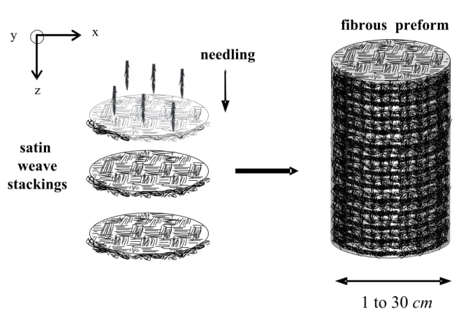
The material we have studied is a C C composite, provided by Snecma Propulsion Solide1. The different steps of the fabrication of its fibrous reinforcement are suggested in figure 1.
1
Weave layers are stacked (xy plane). Then, harpoon-shaped needles are used to punch these cloth stacks : as a consequence, fibers are broken and partially transferred in the z direction .
The stacks are now held together by needlings. The volume fraction of fibers is about 30 %, and 4 % lie in the z orientation. The diameter of carbon fibers is about 8 m. The yarn, less than 1 mm in diameter, is made up of the gathering of a large number of fibers. In this study,
pores inside a yarn will be referred to as micro-pores while pores between yarns will be called macro-pores. Thus, there are two scales of heterogeneity to take into account in order to assess correctly the properties of the preform. Three samples were extracted from the preform at different stages of infiltration. The first one, CC0, was taken from the raw preform. Its bulk density, measured by weighing and measuring the sample, is 470 kg m 3, and the corresponding porosity is 73 %. Two other samples were taken after the preform was partially infiltrated. Owing to the fabrication process (isothermal isobaric CVI), the core of the preform is more porous than its borders. The samples, extracted at different depths, have consequently distinct characteristics. CC1 has a bulk density of 770 kg m 3 (corresponding to 58 % porosity) and CC2 a bulk density of 1520 3
kg m
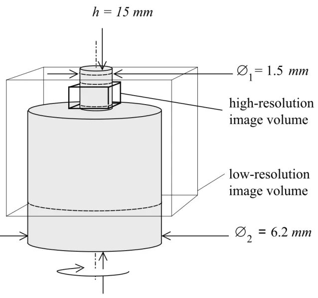
(corresponding to 20 % porosity). The samples were embedded in organic resin and manufactured according to the plan of the figure 2. Their geometry is cylindrical, with a large-section part (bottom) and a narrower part (top), so as to image them at two different resolutions (high and low), and view the two length scales of pore structure.
2.2. Data acquisition and image processing
Tomographic experiments were performed at the ID19 line of the European Synchrotron Radiation Facility (ESRF) in Grenoble [34,35].
2.2.1. High-resolution images
High-resolution images of the upper part of the samples were acquired, with a beam energy of 15 keV ( 0 8339 Å). The sample was positioned with a precise goniometer (fine rotation and translation) and a set of 2D radiographs was recorded every 0.12 of rotation along the vertical axis (up to 180). The average exposure time was 1 s per projection and a complete
acquisition lasted about 35 minutes. 1500 radiographs were recorded on a 2048 2048 CCD-based detector [36] with effective pixel size 0.7 0.7 2
m
. A region of interest of 2048 1024 pixels was selected on the camera so that the size of the reconstructed image is 2048 2048 1024 voxels (corresponding to1.4 1.4 0.7 3
mm ). Reconstruction has been
performed using filtered back-projection [28].The synchrotron X-ray beam on this line, devoted to high-resolution imaging, shows a high lateral coherence due to the small source size and its large distance to the experimental hutch. It gives rise to a phenomenon called phase contrast [37-39], which underlines the interfaces between components of the material. In addition, the low X-ray absorption coefficient of carbon and the reduced length of the absorption path ( 2
mm ) yield a very poor absorption contrast ; as a consequence, only the phase contrast patterns
are present in the reconstructed images. A specific treatment, devised and used by Vignoles [40] on similar images, was used to separate the solid phase, constituted by the fibers and possibly the deposit when the composite is infiltrated, from the pore space. lorblackThe processing procedure is the following :
Application of a double thresholding, i. e., labelling of every node with one of the following three colors : white, gray, and black. The white pixels are considered as fluid, the black ones as solid, and the gray ones are undeterminate at this point.
Application of one or two passes of hysteresis, i. e., a dilation of black and white regions inside the gray region.
labelled.
Each gray connected component is colored according to the color of its skin, that is, the average color of the black and white pixels which are adjacent to it.
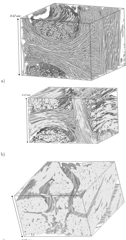
This segmentation procedure was applied to a 800 800 600 cubic voxels extract from CC0. A 3D rendering of the result is shown in figure 3a. A 1296 1120 616 voxels extract from
CC1 was segmented olorblackusing the same algorithm and a partial 3D visualization is shown
in figure 3b. A 1000 1000 600 voxels extract from CC2 was also segmented and the result obtained is shown in figure 3c. These high-resolution images enable us to view the carbon fibers in detail, and are large enough to visualize a few yarns and needlings. However, the size of the investigated area is too small to see the full organization of the yarns and needlings inside the composite. In order to visualize them, images with a lower resolution were acquired. 2.2.2. Low-resolution images
Low-resolution images of the whole sample were acquired with a beam energy of 15 keV ( 0 8339 Å). The sample was positioned with a precise goniometer (fine rotation and translation) and 2D radiographs were recorded every 0.2 of rotation along the vertical axis (up to 180). The average exposure time was 1 s per projection and a complete acquisition lasted
about 25 minutes. 900 radiographs were recorded on a 2048 2048 CCD based detector [36] whose effective pixel size was 7.46 7.46 2
m
. A region of interest of 855 1024 pixels was selected on the camera so that the size of the reconstructed image is 855 855 1024 voxels (corresponding to 6.4 6.4 7.6 3
mm ). The phenomenon of phase-contrast is much less
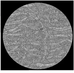
pronounced than in high resolution, but is still visible. On the other hand, absorption contrast is better, since the absorption path (i.e., the sample width) is larger. 2D slices, perpendicular to the rotation axis, and extracted from the reconstructed images of CC0, CC1 and CC2 are shown in figure 4a-c. The resolution allows to view the different components of the fibrous
reinforcement (see figure 4d), and the size of the imaged area is large enough to see numerous yarns and needlings.
3. Computational methods for geometrical characteristics
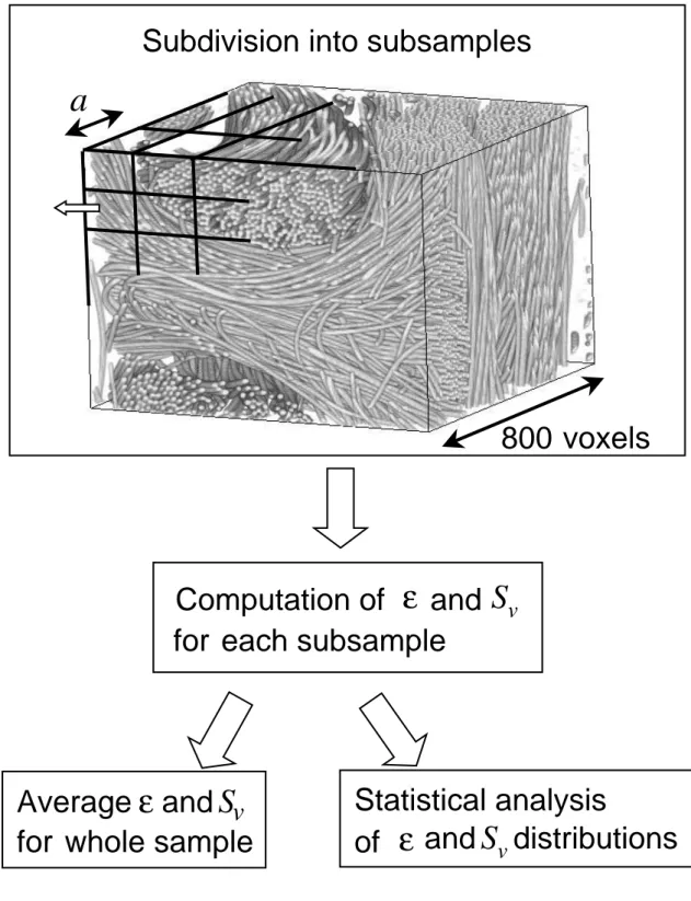
In order to compute easily the geometrical properties (porosity and internal surface area) of the relatively large segmented high-resolution images (made of 5 10 8 voxels each), the procedure described below has been followed (see figure 5):
- Subdivision of the segmented image into cubic sub-samples of edge length a
(variable parameter).
- Computation of the porosity ( ) and the internal surface area (S ) of each v
sub-sample.
- Computation of the mean porosity and mean internal surface area, and
statistical study of distributions.
Details on the local surface area determination are given in the first subsection. The following parts are devoted to the correspondence between low- and high-resolution scans of the same sample, and finally to the determination of the localfiber orientation.
3.1. Surface area evaluation
Porosity can easily be determined from images in which the solid phase is separated from the fluid one. It is simply the ratio between the number of voxels belonging to the fluid phase and the total number of voxels. To compute the internal surface area, we have to consider the interface separating the two phases. A naive choice for this interface would be to consider voxels as cubes : this gives a rather correct evaluation of pore volume fractions, but not for surface area. For instance, the approximated surface of a cylinder parallel to a principal axis would be equal to the surface of the embedding parallelepiped. On the other hand, a full
Marching-Cube method [41] has a rather high computational cost. An intermediate solution, lighter than Marching-Cube and preserving a correct grid convergence for surface area, has been designed [42]. It consists in constructing the walls with triangles whose summits are the interface nodes in 26-connectivity which belong to the solid phase (that is, black nodes of which at least one of their 26 neighbors is white). The effect of this algorithm is to provide a set of connected triangles with Miller indices hkl with (h k l )
1 0 1
3, without any hole between solid and fluid phases. The sum of the triangle areas yields the internal surface area, and the triangles may also be used efficiently for random-walk computations.3.2. Micro-macro correlation
The assessment of the local fiber orientation from CMT scans makes use of the low-resolution images, since this quantity has to be sampled on volumes larger than the reconstructed volumes acquired at high resolution. A porosity correspondence has been established between the low-resolution images and the measured porosity data. The following procedure has been used :
Selection of a 500 voxel size extract in the low-resolution image, 3
Determination of a threshold grayscale value G such that image binarization t
yields the same porosity as measured experimentally, Subdivision of the image into sub-images,
Computation of the porosity inside each sub-image using threshold i G , and t
of the mean value of the grayscale levels G i,
Determination of the linear correlation between and i G i.
The obtained correlation may be used directly at pixel scale ; it has been checked that the average porosity of the sample volumes that have been scanned with both resolutions is the same from either high-resolution and low-resolution procedures.
3.3. Local fiber orientation evaluation
The local orientation of the fibrous medium is not a punctual quantity, i. e., it is intrinsically an average on some volume with a given size. Fortunately, the studied media belong to the case of long, roughly parallel fibers, so that the sensitivity of the local orientation vector to the averaging volume size is not large. As soon as a sampling volume contains enough information concerning the fiber orientation, and until the volume side size becomes as large as yarn curvature, the result is satisfactorily constant with respect to sampling volume.
Many methods exist for anisotropy detection and quantification, based on image gradient processing [43,44], Fourier analysis [45], etc …Rather than using these mathematically elaborate methods, it has been chosen touse a method derived from physics modelling. Indeed, homogenization, volume averaging, or any other change-of-scale theory, when applied to any transport phenomenon, give as a result a tensorial effective transport property, usually a symmetrical second-order tensor in an arbitrary 3D porous medium. The effective tensor coefficients are obtained with a suitable resolution of a local problem – in particular, one has to preserve the orientation, a constraint which excludes symmetry boundary conditions. When only the local orientation is needed (i. e., excluding the absolute values of the transport coefficients), it is possible to use a «degraded» version of the transport properties solvers that will be presented in companion papers, able to yield rapidly a local tensor on a sub-image a few pixels wide, and extract orientation from this tensor. Satisfactory results were obtained with a Monte-Carlo random-walk solver for Knudsen diffusion [42,46]. Each grayscale sub-image was arbitrarily thresholded to 50% porosity – such a processing preserves the anisotropy information – and a set of random walkers was allowed to travel from wall to wall in the «fluid» phase. When a walker exits the sub-image, it is arbitrarily replaced in the fluid phase of the opposite face, with a transmission probability correction which guarantees that transport is not biased by the porosity difference of opposite faces.
The covariance matrix of the centered displacements divided by the walk time converges to a pseudo-diffusion tensor, which is symmetrical and provides the desired information. Summarizing, the local orientation detection has been performed using the following procedure :
Subdivision of the image into 6 voxel size sub-images. 3
Utilization of the random-walk algorithm sensitive to the local anisotropy, yielding a pseudo-diffusion tensor.
Extraction of the principal axes (eigenvectors) and eigenvalues of the pseudo-diffusion tensor. The largest eigenvalue indicates the direction of preferred pseudo-diffusion, which is assimilated to the local fiber orientation.
The scalar product of the local fiber orientation with the three unit vectors x , y and z is computed and the largest value indicates whether the local value is
preferentially x , y, or z ;
The amount of fibers lying preferentially in x , y, or z is computed using a
weighting by the local value of (1i) for the raw sample, and by
0
(1i)(1 ) (1 ht) in a infiltrated sample (where is the raw sample 0
porosity and is the infiltrated sample average porosity).
The orientation vectors defined on all sub-images also define an approximation of a vector field that will be used for the assessment of transport properties.
4. Geometrical characteristics : results and discussion
Images of 3 samples, more or less infiltrated, have been acquired. It has been pointed out that the size of high-resolution images was not large enough to be representative of the full organization of yarns and needlings inside the composite. However, they contain at least one or
two yarns and enable to clearly visualize carbon fibers. Consequently, these high-resolution images will be used in this paragraph to determine structural properties of the composite. These characteristics are total porosity, size distribution between micro and macro-pores, and the internal surface area. Gas transport inside the porous media is directly influenced by porosity while kinetics of heterogeneous chemical reactions are proportional to internal surface area. Results for total or average quantities, as well as statistical distribution for local values are presented, compared with experimental data and discussed.
4.1. Total porosity
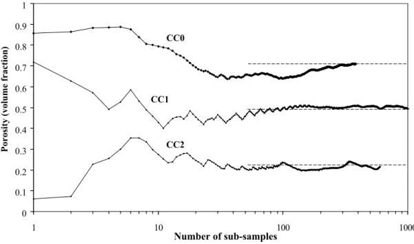
The average porosity of the three segmented images has been computed following the procedure described above, the value of the parameter a being successively set to 100 voxels
and to 32 voxels. Before comparing the porosity average of the image with theporosity measured in the whole sample, it has been checked that the image was large enough to be representative of the porosity of the sample. The variation of the image porosity with the number of sub-samples (a 100) taken for the computation is plotted in figure 6 : when the number of sub-samples is superior to 200, the fluctuations of the porosity are weak, so it can be considered that the corresponding volume ( 0.069 3
mm ) is an REV (Representative
Elementary Volume) for the porosity. The computed porosity can consequently be compared to the porosity measured experimentally in the whole sample. These measurements were realized by weighing the samples and using the following formula:
(1 )
f f f pyC
(1)
where :
: density of partially infiltrated preform
: volume fraction of fibers f
: density of fibers f
pyC : density of the deposit (pyrocarbon or pyC)
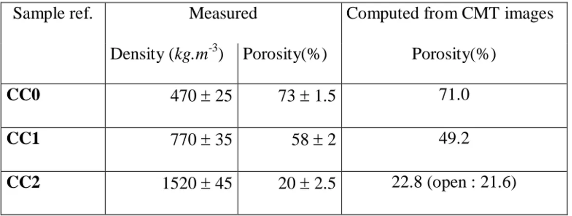
The results obtained are summarized in table 1. There is a good agreement between the experimental data and the computed values. The maximum error is encountered with sample
CC1. However, the segmented volume was intentionally selected in a less porous area so as to
visualize yarns and needlings. Consequently, we can assume that the segmentation of the images, which seemed to be qualitatively good (see figure 3), is actually correct. While the first two samples only do have open porosity, sample CC2 displays an appreciable amount (1.2 %) of closed (inaccessible) porosity.
4.2. Pore size histogram
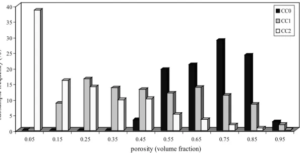
From computed values of sub-sample porosity, it is easy to plot the pore size repartition histogram. The result is dependent on the value of the parameter a . When a is equal to 100
voxels (70 m), the histogram of figure 7 is obtained. In the raw state (sample CC0), the porosity is nearly uniformly distributed between 50 and 90 %. The image is not subdivided into sufficiently small sub-samples so that the macro-pores can be separated from micro-pores. In the slightly infiltrated state (sample CC1), the porosity is distributed between 10 and 90 %. There are two populations of sub-samples: one having a mean porosity of 25 %, and the other 65 %. The first one corresponds to micro-porous sub-samples, the second one to macro-porous sub-samples. These two populations have, at this stage of infiltration, sufficiently different pore sizes so that they can be distinguished from each other on the histogram. In the more infiltrated state (sample CC2), the main part of sub-samples, which has less than 10 % of porosity, contains micro-pores. The second population, associated to the macro-pores, has a mean porosity of 45 %. This histogram enables us to visualize the way the pore space is distributed
and how it evolves with infiltration. However, the sub-sample size is not fine enough to allow to distinguish clearly the two populations of sub-samples (micro and macro-porous), especially in the raw state.
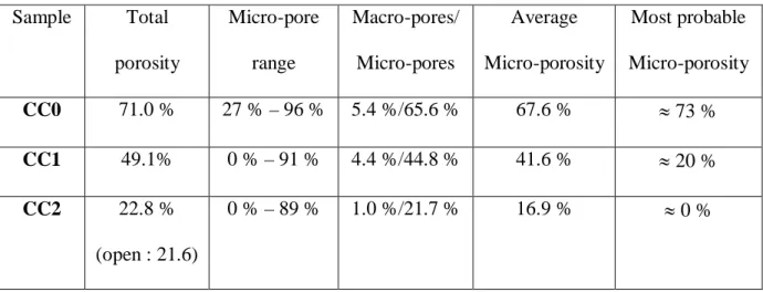
The pore volume distribution obtained with parameter a equal to 32 voxels (22.4 m) is shown in figure 8. This sampling allows to distinguish better the two sub-sample populations. Results obtained by separating the porepopulation into two subsets are summarized at table 2. In the raw state (sample CC0), sub-samples are distributed between a totally void population and a population having a mean porosity of 68 %. The first one is constituted by sub-samples taken from macro-pores whereas the second one is constituted by sub-samples located inside needlings or yarns. The micro-porous population is relatively spread (between 25 and 96 %). This is probably due to the fact that yarns and needlings do not have the same average porosity; in addition, the size of the sampling 3-dimensional window ( 3
a ) broadens the distribution. In
the slightly infiltrated state (sample CC1), the micro-porous population has an average porosity of 43 %, but with a mode at 15 %. The percentage of macro-porous sub-samples is, as for CC0, not much different from the initial percentage. This shows that the deposit, in the initial stages of infiltration, occurs mainly in the micro-pores. This is due to the high specific surface developed inside the yarns and the needlings. In the most infiltrated state (sample CC2), the micro-pore distribution is completely shifted towards low values. At this stage, deposition occurs around the yarns and the needlings since micro-pores are now poorly accessible. We can notice that the infiltration of yarns and needlings stops (because there are no more accessible micro-pores) at an intermediate stage between CC1 and CC2. After that moment, deposition occurs principally in the macro-pores, as can be seen in the macro-porosity evolution in Table 2. It has already been mentioned that the filling of macro-pores, which do not have an important internal surface area, often constitutes the most important part (in time) of the infiltration [32]. However, in this precise case, the macro-pore volume has already somewhat
decreased (seethe decreasing of the percentage of macro-porous sub-samples in table 2 between
CC0 and CC1) so that it will not require a very long time to finish filling them. The structure
of the preform studied here seems thus well suited to infiltration by CVI.
4.3. Average internal surface area
The procedure described in paragraph 1 has been applied to the computation of the internal surface area of each sub-sample of the images of CC0, CC1 and CC2 (with parameter a equal
to 100 voxels).The total surface area is then obtained by summing up the values from all sub-samples. In the same way as for porosity, we checked that the volume of the image was large enough to be representative of the internal surface area of the wholesample. Additionally, the internal surface area of the preform was measured experimentally by BET krypton adsorption on three samples. The results are shown in figure 9. The samples taken for the experimental measurements were not the same as for the calculations from images. This explains the difference of the porosity between the samples characterized experimentally and numerically. It may be noticed that the computed values are appreciably inferior to the experimental ones for the less infiltrated samples, whereas this difference seems to decrease with the infiltration. Such a difference arises from the limited resolution of the 3D CMT images, as compared to physical adsorption : any detail inferior to 1 m is ignored. Thus the surface of the fiber appears smooth whereas a SEM micrograph shows that there is a neat roughness at a finer scale ( 0.2
m
) (see figure 10a). However, this roughness progressively decreases,as the pyrocarbon deposit grows (see figure 10b) : that is the reason why there is much less difference between measured and computed values in the final stages of infiltration.
4.4. Internal surface area/porosity correlations
CC1 and CC2 have been computed, it is possible to study the correlation between these
quantities and compare it to formulæ obtained for ideal structures :
1. Non-overlapping cylinders of radius r of any orientation distribution. For such
a structure, whatever the relative orientation of the fibers, the correlation is:
2 1 v S r (2)2. - Random array of freely overlapping cylinders of radius r of any orientation distribution. In this case, Tomadakis and Sotirchos [12] suggested to use the following equation, which is in good agreement with their simulations:
2 ln v S r (3)3. - Random array of parallel (1D) cylinders with partial overlapping. One of the ways to construct such a structure was described by Tomadakis and Sotirchos [7]. A random array of non-overlapping fibers of porosity 0 is constructed first : cylinders of
radius r0 are placed on the nodes of a hexagonal array, then moved randomly numerous
times, with their new positions rejected if the cylinders overlap. Beds of partially overlapping fibers are obtained by allowing the cylinder radius to grow from r0 to r
(with the cylinder growth representing the material deposited on the fibers during infiltration). The correlation between the porosity and the internal surface of this structure was established by Rikvold and Stell [11,47]:
0 0 0 2 1 1 1 1 v S r (4)
2 2 2 0 0 0 1 1 exp 1 1 1 1 (5) 0 r r (6)In order to determine which model structure best approximates the real preform, the internal surface area of each sub-sample has been plotted versus its porosity (figure 11). For sample
CC0, the relation between the internal surface area and the porosity is linear and matches
equation (2), the best fit (R2 = 0.989) is obtained with a cylinder radius of 3.98 µm, i. e., practically identical to the actual fiber radius. The standard deviation of the fiber radius distribution is 0.14 µm, i.e. 3.5%, a very narrow distribution. This means that, as expected, the fibers can be considered as cylindrical and of uniform radius. For partially infiltrated samples (CC1 and CC2), the relation between Sv and is quite different. Due to the solid deposit
around the fibers, they now appear to be partially overlapping. A series expansion to first order in (1-) of equations (4-5) yields the following approximation for Sv = f(1-):
0 2 1 v S r (7)which is nothing else than a combination of eqs. (2) and (6). A least squares fitting on the high-porosity data points yields a value of = 1.65 0.2 with correlation factor R2 = 0.989 : this is consistent with direct measurements on selected fibers in the SEM image and on CMT slices. Consequently, in order to model the results for CC1, all data points of CC0 have been transformed through use of equations (4-5), with set to 1.65. It can be seen on figure 11 that
the transformed distribution according to the model of Rikvold and Stell is very similar to the actual CC1 sample distribution, though narrower. A conclusion of this study is that the 1D fiber growth model accounts well for the actual arrangement of fibers, despite some scattering, probably due to the fact that the fibers are not strictly parallel, and to the presence of macro-pores. For CC2, a correlation of the same form was found for the open porosity, with equal to
3.6. For such a value of , equation (4) is very close to equation (3). Both laws are relatively
good models for the behavior of the real fibrous structure. At this stage of infiltration, there are closed pores so that the parameter is not constant throughout the sample. Moreover the
diameter of pores is often of the order of a few pixels, and an error is encountered in the computation of and Sv in particular. This can explain why there is also some scattering around
the correlation for sample CC2.
4.5. Pore size distributions
When pore volume and internal surface are known for any image or sub-image, the average local pore diameter may be estimated using the classical formula 48:
4 p v d S (8)
Doing so, it has been possible to evaluate the distributions of pore diameters in the CMT images. Results are presented as incremental volume per unit mass of sample, so that they may be directly compared with mercury intrusion data. Samples different from the three previous ones, but originated from the same infiltration run on the same preform, have been used for the experimental determination of pore size distribution by mercury intrusion. It was not possible to study experimentally a raw sample, because of its mechanical weakness. Figure 12 is a comparative plot of the five distributions. Several remarks arise from this figure :
The macro-pore sizes are much larger for the experimental data, for two reasons : (i) the sample size was larger, and (ii) the size estimation for the computed distribution is limited by the sub-sample dimensions (70 µm), so the macro-pore estimated distribution ranges «artificially» between 40 and 140 µm, as suggested by the arrow on the graph2. Of course, increasing parameter a would give better estimates of the macro-pore dimensions, but on the other hand,the noise on the whole distribution function – already much larger than for mercury intrusion data – would be larger.
The micro-pore size distributions are in good agreement : the 46% porosity
2
It is not surprising that the largest pore size estimation may be as high as twice the edge dimension – just apply formula (8) to a cube containing only fluid phase, and fluid/solid
sample studied experimentally, and the 50% porosity sample studied from CMT are in close agreement in the 10-30 µm range, and the evolution of the curves for the five samples is coherent.
4.6. Local fiber orientation
The assessment of the local fiber orientation from CMT scans makes use of the low-resolution images. The computational procedures for porosity correlation and orientation detection have been applied successively to samples CC0 and CC1. The procedures have not been applied to sample CC2 : indeed, the micro-pores are so small that the anisotropy information is lost at the sub-image size. Qualitative results are shown in figure 13 on CMT slices of samples CC0 and
CC1. Quantitative results for three image extracts are shown in table 3, where the experimental
x, y, and z fiber fractions have been also reported for comparison. The experimental
determination of the preferred fiber orientation is described in [49] and has been applied to the same preforms. Some remarks arise from these results :
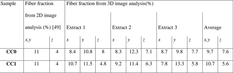
There is some variation in the determined values from one extract to the other : this is due to the fact that the REV size is probably larger than the extract size.
The z fiber fraction is larger in the CMT procedure than in the previous work : evidently, in this work some more parts of the woven textile are recognized as lying along z, relative to those found in the 2D procedure.
A small but perceptible difference, not measured in the preceding work, exists between x and y fiber fractions : indeed, the y direction is the weave direction and weave threads are less subject to off-axis distortions than warp (x) threads.
interface on only two faces.
5. Conclusion
A C/C composite at various infiltration stages has been imaged by Computerized Micro-Tomography (CMT) for the first time at high resolution, enough to distinguish clearly individual fibers present in it. From high-resolution images of a preform, and provided an efficient segmentation is performed, it is possible to quantify the way the pore volume is distributed between micro and macro-pores. Various indicators of the geometrical characteristics of the porous space have been produced and compared to experimental data : porosity, internal surface area, surface-to-porosity correlation and distributions of pores and preferred local fiber orientation. These indicators have been monitored as a function of the infiltration. Up to the limitations inherent to direct imaging (i.e. image size and resolution), the results are in fairly good agreement with experimental data. This validates the whole study as an efficient tool for quantitative parameter estimation from direct 3D imaging. Also, it is shown that the studied fiber architecture has good infiltrability qualities, that is, it is able to receive a large amount of matrix by Chemical Vapor Infiltration. Many directions may be sought from the starting point provided here. First, it would be very interesting to do the same computations in other kinds of preforms and compare the results with those of this study. Second, a more evolved segmentation procedure should be devised in order to separate the matrix from the fibers at high resolution : this would increase the quality of some estimations. Third, many computations and simulations are possible on the basis of validated 3D images of a given porous medium, especially because a double change-of-scale strategy is provided. A companion article will present results on this strategy and the computed heat and mass transport properties.
Acknowledgements
authors are also indebted to the ID 19 team (José Baruchel, Peter Cloetens, Elodie Boller, and others) for their assistance during CMT data acquisition. Jean-Marie Vallerot (LCTS) is acknowledged for providing the SEM micrographs of figure 10.
References
[1] R. Naslain and F. Langlais : Fundamental and practical aspects of the chemical vapor infiltration of porous substrates. High Temperature Science, 27, 221 (1990).
[2] T. L. Starr : Modeling of forced flow-thermal gradient CVI. In Proc. of International Conference on Whisker and Fiber-Thoughened Ceramics, edited by R. A. Bradley, D. E. Clark , D. S. Larsen and J. Q. Stiegler (ASM International, Metals Park, OH, 1988), p. 243.
[3] P. McAllister and E. E. Wolf : Simulation of a multiple substrate reactor for chemical vapor infiltration of pyrolytic carbon within carbon-carbon composites. AIChE J. 39, 1196 (1993). [4] G. L. Vignoles, C. Descamps, and N. Reuge : Interaction between a reactive preform and the surrounding gas-phase during CVI. In Euro-CVD 12 Proceedings, edited by A. Figueras (J.
Phys. IV France 10, EDP Sciences, Les Ulis, France, 2000) p. Pr2-9.
[5] N. Reuge and G. L. Vignoles : Global modelling of I-CVI : Effects of reactor control parameters on a densification. J. Mater. Proc. Technol., in press, (2004).
[6] D. Leutard, G. L. Vignoles, F. Lamouroux, and B. Bernard : Monitoring density and temperature in C/C composites elaborated by CVI with radio-frequency heating. J. Mater.
Synth. and Proc. 9, 259 (2002).
[7] M. M. Tomadakis and S. V. Sotirchos : Knudsen diffusivities and properties of structures of unidirectional fibers. AIChE J. 37, 1175 (1991).
[8] T. L. Starr and A. W. Smith : Advances in modeling of the forced chemical vapor infiltration process. In Chemical Vapor Deposition of Refractory Metals and Ceramics II, edited by T. M. Besmann, B. M. Gallois, and J. W. Warren, (Mat. Res. Soc. Symp. Proc. 250, Pittsburgh, PA, 1992). p. 207.
[9] M. M. Tomadakis and S. V. Sotirchos : Transport properties of random arrays of freely overlapping cylinders with various orientation distributions. J. Chem. Phys. 98, 616 (1993). [10] J. Y. Ofori and S. V. Sotirchos : Structural model effects on the predictions of CVI
models. J. Electrochem. Soc. 143, 1962 (1996).
[11] P. A. Rikvold and G. Stell : d-dimensional interpenetrable-sphere models of random two-phase media : microstructure and an application to chromatogaphy. J. Coll. Int. Sci. 108, 158 (1985).
[12] M. M. Tomadakis and S. V. Sotirchos : Effective Knudsen diffusivities in structures of randomly overlapping fibers. AIChE J. 37, 74 (1991).
[13] W. T. Perrins, D. R. McKenzie, and R. C. McPhedran : Transport properties of regular arrays of cylinders. Proc. R. Soc. Lond. A 369, 207 (1979).
[14] G. W. Milton : Bounds on the transport and optical properties of a two-component composite material. J. Appl. Phys. 52, 5294 (1981).
[15] D. S. Tsai and W. Strieder : Effective conductivities of random fiber beds. Chem. Eng.
Commun. 40, 207 (1986).
[16] J. F. McCarthy : Effective conductivity of many component composites by a random walk method. J. phys. A : Math. Gen. 23, L445 (1990).
[17] I. C. Kim and S. Torquato : Determination of the effective conductivity of heterogeneous media by brownian motion simulation. J. Appl. Phys. 68, 3892 (1990).
[18] M. M. Tomadakis and S. V. Sotirchos : Transport through random arrays of conductive cylinders dispersed in a conductive matrix. J. Chem. Phys. 104, 6893 (1996).
[19] S. Torquato and J. D. Beasley : Effective properties of fiber-reinforced materials : I. Bounds of the effective thermal conductivity of dispersions of fully penetrable cylinders. Int. J.
Eng. Sci. 24, 415 (1986).
[20] C. G. Joslin and G. Stell : Effective properties of fiber-reinforced composites : Effects of polydispersity in fiber diameter. J. Appl. Phys. 60, 1611 (1986).
[21] R. R. Melkote and K. F. Jensen : Computation of transition and molecular diffusivities in fibrous media. AIChE J. 38, 56 (1992).
[22] M. M. Tomadakis and S. V. Sotirchos : Ordinary and transition regime diffusion in random fiber structures. AIChE J. 39, 397 (1993).
[23] F. G. Ho and W. Strieder : Asymptotic expansions of the porous medium effective diffusivity coefficient in the Knudsen number. J. Chem. Phys. 70, 5635 (1979).
[24] T. L. Faley and W. Strieder : Knudsen ow through a random bed of unidirectional fibers.
J. Appl. Phys. 62, 4394 (1987).
[25] R. R. Melkote and K. F. Jensen : Gas diffusion in random fiber structures. AIChE J. 35, 1942 (1989).
[26] A. S. Sangani and A. Acrivos : Slow ow past periodic arrays of cylinders with application to heat transfer. Int. J. Multiphase Flow 8, 193 (1982).
[27] J. F. McCarthy : Analytical models for the effective permeability of sand-shale resevoirs.
Geophys. Int. J. 105, 513 (1991).
[28] A. C. Kak and M. Slaney : Principles of computerized tomographic imaging. (Electronic version, Classics in Applied Math. 33, SIAM, 2001).
[29] J. Baruchel, J.-Y. Buffière, E. Maire, P. Merle, and G. Peix : X-ray tomography in material science. (Hermès Science Publications, Paris, 2000).
[30] G. Y. Baaklini, R. T. Bhatt, A. J. Eckel, P. Engler, M. G. Castelli, and R. W. Rauser : X-ray microtomography of ceramic and metal matrix composites. Materials Evaluation 53, 1040 (1995).
[31] J. Kim, P. K. Liaw, D. K. Hsu, and D. J. McGuire : Nondestructive evaluation of
Nicalon/SiC composites by ultrasonics and X-ray computed tomography. In Proc. 21st Annual Conference and Exposition on Composites, Advanced Ceramics, Materials and Structures,
edited by J. P. Singh, (Ceram. Eng. Sci. Proc. 18, Westerville, OH, 1997), p. 287.
[32] J. H. Kinney, T. M. Breunig, T. L. Starr, D. Haupt, M. C. Nichols, S. R. Stock, M. D. Butts, and R. A. Saroyan : X-ray tomographic study of chemical vapor infiltration processing
of ceramic composites. Science 260, 789 (1993).
[33] S-B. Lee, S. R. Stock, M. D. Butts, T. L. Starr, T. M. Breunig, and J. H. Kinney : Pore geometry in woven fiber structures : 0°/ 90°plain-weave cloth layup preform. J. Mater. Res. 13,
1209 (1998).
[34] J. Baruchel : Topography and high-resolution diffraction beamline ID 19. In ESRF
Beamline Handbook, edited by R. Mason (ESRF User Office, Grenoble, 1995) p. 115.
[35] J. Baruchel and J. Härtwig : ID 19 topography and high-resolution diffraction handbook. http://www.esrf.fr/exp facilities/ID19/handbook/handbook.html (2004).
[36] J. C. Labiche, J. Segura-Puchades, D. Van Brussel, and J. P. Moy : FReLON camera : Fast Readout Low Noise. ESRF Newsletter n° 25, 41 (1996).
[37] M. Ando and S. Hosoya : An attempt at X-ray phase-contrast microscopy. In Proc. 6th
Intern. Conf. On X-ray Optics and Microanalysis, edited by G. Shinoda, K. Kohra, and T.
Ichinokawa, (Univ. of Tokyo Press, Tokyo, 1972) p. 63.
[38] P. Cloetens, M. Pateyron-Salomé, J.-Y. Buffière, G. Peix, J. Baruchel, F. Peyrin, and M. Schlenker : Observation of microstructure and damage in materials by phase sensitive
radiography and tomography. J. Appl. Phys. 81, 5878 (1997).
[39] E. Maire, J.-Y. Buffière, P. Cloetens, G. Lormand, and R. Fougères : Characterisation of internal damage in an MMCp using X-ray synchrotron phase contrast microtomography. Acta
Mater. 47, 1613 (1999).
[40] G. L. Vignoles : Image segmentation for hard X-ray phase contrast images of C/C composites. Carbon 39 167 (2001).
[41] W. E. Lorensen and H. E. Cline : Marching cubes: A high resolution 3D surface construction algorithm. In SIGGRAPH '87 Proceedings, edited by M. C. Stone, (ACM
Computer Graphics 21, ACM Press, New York, NY, 1987), p. 163.
complex porous media. J. de Physique IV, C5, 159 (1995).
[43] E. P. Lyvers and O. R. Mitchell : Precise edge contrast and orientation estimation. IEEE
Trans. on Pattern Analysis and Machine Intelligence 10, 927 (1988).
[44] C. Germain, J. P. Da Costa, O. Lavialle, and P. Baylou : Multiscale estimation of vector field anisotropy application to texture characterization. Signal Process. 83, 1487 (2003). [45] J. Bigün, G. H. Granlund, and J. Wiklund : Multidimensional orientation estimation with applications to texture analysis and optical flow. IEEE Trans. on Pattern Analysis and Machine
Intelligence 13, 775 (1991).
[46] V. N. Burganos and S. V. Sotirchos : Knudsen diffusion in parallel, multidimensional, or randomly oriented pore structures. Chem. Eng. Sci. 44, 2451 (1989).
[47] P. A. Rikvold and G. Stell : Porosity and specific surface for interpenetrable-sphere models of two-phase random media. J. Chem. Phys. 31, 1014 (1985).
[48] C. N. Satterfield : Mass transfer in heterogenous catalysis. Technical Report MA-41, (MIT Press, Cambridge, MA, 1970).
[49] M. Jonard : Study of the pore network of tridimensional textures (in French). Technical report, (Snecma Propulsion Solide, Le Haillan, France, 2001).
Tables
Sample ref. Measured Computed from CMT images Density (kg.m-3) Porosity(%) Porosity(%)
CC0 470 25 73 1.5 71.0
CC1 770 35 58 2 49.2
CC2 1520 45 20 2.5 22.8 (open : 21.6)
Table 1. Pore volume fractions measured and computed from high-resolution CMT images on the three samples
Sample Total porosity Micro-pore range Macro-pores/ Micro-pores Average Micro-porosity Most probable Micro-porosity CC0 71.0 % 27 % – 96 % 5.4 %/65.6 % 67.6 % 73 % CC1 49.1% 0 % – 91 % 4.4 %/44.8 % 41.6 % 20 % CC2 22.8 % (open : 21.6) 0 % – 89 % 1.0 %/21.7 % 16.9 % 0 %
Fiber fraction from 3D image analysis(%) Fiber fraction
from 2D image
analysis (%) [49] Extract 1 Extract 2 Extract 3 Average Sample
x,y z x y z x y z x y z x,y z
CC0 11 4 8.4 10.8 8 8.3 12.3 7.1 8.7 9.8 7.7 9.7 7.6
CC1 11 4 10.7 11.5 4.8 9.2 11.4 6.3 7.8 13.3 5.8 10.7 5.6
Figure Captions
Figure 1 : Fibrous organization of the preform, made of a stacking of satin weaves that are punched by needles.
Figure 2 : Sample geometry and location of the scanned areas.
Figure 3 : 3D renderings of extracts from reconstructed and segmented images CC0 (a), CC1 (b) , and CC2 (c).
Figure 4 : 2D visualizations of low-resolution tomographic slices extracted from CC0 (a), CC1 (b) , and CC2 (c) and visualization of yarns and needlings in sample CC1 (d).
Figure 5 : Computational method for the evaluation of geometrical characteristics. Figure 6 : Convergence of porosity evaluation with respect to sample volume.
Figure 7 : Porosity repartition histogram between sub-samples of edge size a = 100 voxels. Figure 8 : Porosity repartition histogram between sub-samples of edge size a = 100 voxels. Figure 9 : Comparison of experimental and computed internal surface areas.
Figure 10 : SEM fiber-scale imaging of samples with 70% porosity (a), and 36% porosity (b). Figure 11 : Correlation plot of internal surface area and local porosity for the three samples. Transformed distributions of CC0 and other theoretical predictions are also plotted.
Figure 12 : Pore size distributions from mercury penetration and from 3D image analysis. Figure 13 : Local fiber orientation results on slices of sample CC0 (a) and CC1 (b).
Table Captions
Table 1 : Porosities measured and computed from high-resolution CMT images on the three samples.
Table 2 : Statistical data extracted from the distributions of figure 8. Table 3 : Fiber orientation results.
Figures
fibrous preform
needling
x z ysatin
weave
stackings
1 to 30 cm
Figure 1: Fibrous organization of the preform, made of a stacking of satin weaves that are punched by needles
∅
2
= 6.2 mm
∅
1
= 1.5 mm
h = 15 mm
low-resolution
image volume
high-resolution
image volume
Figure 2: Sample geometry and location of the scanned areas
a)
b)
c)
Figure 3: 3D renderings of extracts from reconstructed and segmented images CC0 (a), CC1 (b) , and CC2 (c)
a) b) 1 mm x z y Needling Warp yarn Weft yarn c) d)
Figure 4: 2D visualizations of low-resolution tomographic slices extracted from CC0 (a), CC1 (b) , and CC2 (c) and visualization of yarns and needlings in sample CC1 (d).
a
800 voxels
Subdivision into subsamples
Computation of
ε
and
S
v
for each subsample
of
ε
Statistical analysis
and
S
v
distributions
ε
and
S
for
v
Average
whole sample
Figure 5: Computational method for the evaluation of geometrical characteristics.
0 0.1 0.2 0.3 0.4 0.5 0.6 0.7 0.8 0.9 1 1 10 100 1000 Number of sub-samples CC0 CC1 CC2 P or os
ity (volume fraction)
Figure 6: Convergence of porosity evaluation with respect to sample volume.
0 5 10 15 20 25 30 35 40 subsample frequency (% ) 0.05 0.15 0.25 0.35 0.45 0.55 0.65 0.75 0.85 0.95
Répartition de la porosité des différents échantillons
CC0 CC1 CC2
porosity (volume fraction)
Figure 7: Porosity repartition histogram between sub-samples of edge size a = 100 voxels
0 0.5 1 1.5 2 2.5 3 0 0.2 0.4 0.6 0.8 1
sub-sample number frequency (%)
CC0 (porosity : 71.0%) CC1 (porosity : 49.2 %) CC2 (porosity : 21.6 %)
micro macro
porosity (volume fraction)
Figure 8: Porosity repartition histogram between sub-samples of edge size a = 32 voxels
0 50000 100000 150000 200000 250000 0.2 0.3 0.4 0.5 0.6 0.7 0.8 in te r n al s u r fac e ar e a ( m )
Computed from 3D images Kr BET measurements
-1
porosity (volume fraction)
Figure 9: Comparison of experimental and computed internal surface areas
a)
Carbon
fiber
pyC deposit
b)Carbon
fiber
pyC deposit
Figure 10: SEM fiber-scale imaging of samples with ≈ 70% porosity (a), and ≈ 36% porosity (b)
0 0.05 0.1 0.15 0.2 0.25 0 0.2 0.4 0.6 0.8 1
Porosity (volume fraction)
CC0 Growth from CC0, δ = 1.41 in eqs. (4-5) CC1 Growth from CC0, δ = 3.14 in eqs. (4-5) CC2 Linear approx. , δ = 1.65 in eq. ( 7) Random cylinders, δ = 3.6 in eqs. (3,6)
Scaled surface are
a, S * < r > v 0
Figure 11: Correlation plot of internal surface area and local porosity for the three samples. Transformed distributions of CC0 and other theoretical predictions are also plotted.
0 0.02 0.04 0.06 0.08 0.1 0.12 1 10 100 1000 Pore size (µm) Incremental volume (mL/g) Computed, 71% porosity Computed, 50% porosity Measured, 46% porosity Measured, 34% porosity Computed, 23% porosity
Figure 12: Pore size distributions from mercury penetration and from 3D image analysis
x z y x z y a) b) x preferred orientation y preferred orientation z preferred orientation
Figure 13: Local fiber orientation results on slices of sample CC0 (a) and CC1 (b)