HAL Id: ensl-00989760
https://hal-ens-lyon.archives-ouvertes.fr/ensl-00989760
Submitted on 12 May 2014
HAL is a multi-disciplinary open access
archive for the deposit and dissemination of
sci-entific research documents, whether they are
pub-lished or not. The documents may come from
teaching and research institutions in France or
abroad, or from public or private research centers.
L’archive ouverte pluridisciplinaire HAL, est
destinée au dépôt et à la diffusion de documents
scientifiques de niveau recherche, publiés ou non,
émanant des établissements d’enseignement et de
recherche français ou étrangers, des laboratoires
publics ou privés.
Nonnegative matrix factorization to find features in
temporal networks
Ronan Hamon, Pierre Borgnat, Patrick Flandrin, Céline Robardet
To cite this version:
Ronan Hamon, Pierre Borgnat, Patrick Flandrin, Céline Robardet. Nonnegative matrix factorization
to find features in temporal networks. 2014 IEEE International Conference on Acoustics, Speech, and
Signal Processing (ICASSP), May 2014, Florence, Italy. pp.SPTM-P4.1. �ensl-00989760�
NONNEGATIVE MATRIX FACTORIZATION TO FIND FEATURES IN TEMPORAL
NETWORKS
Ronan Hamon , Pierre Borgnat, Patrick Flandrin
Physics Laboratory, CNRS UMR 5672
ENS Lyon, Universit´e de Lyon
Lyon, France
[email protected]
C´eline Robardet
LIRIS, CNRS UMR 5205
INSA Lyon, Universit´e de Lyon
Villeurbanne, France
[email protected]
ABSTRACT
Temporal networks describe a large variety of systems having a tem-poral evolution. Characterization and visualization of their evolution are often an issue especially when the amount of data becomes huge. We propose here an approach based on the duality between graphs and signals. Temporal networks are represented at each time instant by a collection of signals, whose spectral analysis reveals connec-tion between frequency features and structure of the network. We use nonnegative matrix factorization (NMF) to find these frequency features and track them over time. Transforming back these features into subgraphs reveals the underlying structures which form a de-composition of the temporal network.
Index Terms— nonnegative matrix factorization, temporal net-works, Fourier analysis, dynamic graphs, multidimensional scaling
1. INTRODUCTION
Many systems associated to networks, whether physical, biological or social, can be described by graphs [1]. The study of the structure of these graphs helps us to describe, understand and predict the be-havior of systems. Often, these systems are not frozen but have a time evolution, e.g. associated connections which appear and disap-pear over time, or apparition or disapdisap-pearance of nodes. We study here temporal networks where the edges are changing with times, keeping the same given set of nodes (possibly isolated).
Temporal networks have been introduced and studied in differ-ent fields under various names. Holmes and Saram¨aki [2] proposed a review about temporal networks which includes discussion about the different types of temporal networks, the measures of the struc-ture and the associated models. Casteigts et al. [3] also reviewed some works about dynamic networks with a graph theory approach. Evolving graphs were also considered as models for social networks [4] or networks with information spreading [5]. As for visualization, Xu et al. [6] proposed a method based on multidimensional scaling (MDS). The temporal networks considered in this work consist in a series over time of snapshots of graphs, which are static at a given instant of time.
We propose a new approach based on the duality between graphs and signals to study temporal networks. Duality between graphs and signals consists in the transformation from (static) graphs to signals and inversely, in order to study either signals thanks to graph theory or graphs with signal processing. Campanharo et al. [7] proposed a
This work is supported by the programs ARC 5 and ARC 6 of the r´egion Rhˆone-Alpes
method where the graphs represent a Markov chain coding the sig-nals. Haraguchi et al. [8] and later Shimada et al. [9] proposed a method to transform graphs into time series using classical multidi-mensional scaling (CMDS). We previously extended this approach in order to highlight relations between the structure of a graph and the associated frequency patterns, as well as to visually track tempo-ral networks by following such patterns [10]. This method has been exploited to build approximation of the graph over time with an ap-plication to the study of a bike sharing system in Lyon [11] [12]. The novelty here is to decompose a whole temporal network, first by ob-taining frequency patterns by duality and then by using nonnegative matrix factorization (NMF) [13] to decompose these local spectra of the temporal network into features associated with weights evolving over time.
Section 2 recalls the duality mapping from graphs to signals. In Section 3 we extend the method to temporal networks using NMF and explain how the features are obtained. Section 4 gives an exam-ple on a controlled model of synthetic temporal network. A conclu-sion is given in Section 5.
2. FROM NETWORKS TO SIGNALS
LetG be a simple undirected and unweighted graph with n nodes. We note(Aij)i,j=1,..,nits adjacency matrix.
2.1. Principle
Shimada et al. [9] proposed a method to transform a graph into a collection of signals ofn points indexed by the vertices of the graph by using classical multidimensional scaling (CMDS).
This transformation consists in applying CMDS to a matrix dis-tance between vertices of a graph, noted ∆ = (δij)i,j=1,..,n and
defined for two nodesi, j of G by
δij= 0 ifi = j 1 ifaij= 1 and i 6= j w > 1 ifaij= 0 and i 6= j Following [9], we choosew = 1.1.
Multidimensional scaling (MDS) [14] is a set of mathematical techniques used to represent measurements of dissimilarity among pairs of objects as distances between points in a multidimensional space whose dimension is low. Classical MDS is a particular case of metric MDS where the dissimilarities are assumed to be Euclidean distances. The matrix X of coordinates in the low-dimensional, transformed space can be computed analytically. Starting with the
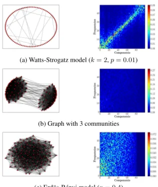
(a) Watts-Strogatz model (k = 2, p = 0.01)
(b) Graph with 3 communities
(c) Erd¨os-R´enyi model (p = 0.4)
Fig. 1. (left) Snapshot of the network. (right) Frequency analysis of the resulting signals. (a) The regularity of the structure of is apparent as high values on the diagonal ofS(k, f ). (b) Structure in commu-nities implies very high magnitudes at low frequencies for the first components. (c) Random structure leads to a spread of magnitudes over all frequencies.
distance matrix ∆, we first compute a double centering of the matrix whose terms are squared : B= −1
2J∆
(2)J with J= I
n−n11n1Tn
where Inis the identity matrix and 1n1Tn an × n matrix of ones.
The CMDS solution is given by X= Q+Λ 1 2
+ with Λ+a diagonal
matrix whose terms are the eigenvalues of the matrix B sorted in an increasing order and Q+is the matrix of the corresponding
eigen-vectors. The resulting signals are the components (or columns) of the matrix X. Thej-th signal is noted X(j).
The inverse transformation from signals to graph is trivial: ac-cording to the principle of the CMDS, the distance matrix D between points in the Euclidean space is equal to the distance matrix ∆. The adjacency matrix A derives clearly from ∆.
2.2. Relabeling of a graph
Shimada et al. [9] showed that ring lattices are transformed into peri-odic signals: each component is a monochromatic oscillation whose frequency depends on the index of the component. More generally, it is relevant to use spectral analysis to link frequency features of sig-nals with graph properties. Spectral analysis is nonetheless closely related to the indexation of signals and so to the labeling of the graph. Finding a good labeling of vertices is therefore essential to avoid sudden variations of signals. That means that it is necessary to have close labeling between neighbor vertices, which are defined closer in the distance matrix than unlinked vertices. This problem can be related to another graph labeling problem called cyclic bandwidth sum problem [15]. We proposed in [16] a heuristic that will be used throughout this paper but not explained further.
# Definition of the steps
1 Transformation ofGtinto a collection of signals Xt
2 Frequency analysis of signals: Vt= |F Xt(f )|
3 NMF: V ≈ W H
4 Identification of features Wkand levels of activation Hk
5 Transformation into a spectrum ˆY = Wk.eiφ
6 Inverse Fourier transformation: Y = F−1Yˆ
7 Transformation from the signals Y to a graphH
Table 1. Procedure of the analysis of a temporal network. Descrip-tion of each step is given in SecDescrip-tion 3.
2.3. Analysis of signals
Let us consider a collection ofK signals indexed by n vertices. We use the amplitude spectrum of the Fourier transform. From the mag-nitude of each frequency for each componentk ∈ {1, . . . , K}, this amplitude reads as:
S(k, f ) = |F X(k)(f )| (1) estimated, for positive frequencies, onF = n
2+ 1 bins, F being the
Fourier transform.
Fig. 1 shows that specific graph properties, such as being regular in degrees (Watts-Strogatz model [1]) or being structured in commu-nities, have specific frequency patterns. A random structure (Erd¨os-R´enyi model [1]) is also visible in the spectrum of the collection of signals as the magnitudes are spread out over all the frequencies.
3. TEMPORAL NETWORK AND NMF
The duality between networks and signals defined in the previous section enables us to link frequency features with graph properties. We propose in this section to extend the transformation towards tem-poral network and use nonnegative matrix factorization (NMF) to catch these features and follow their level of activation over time. We finally exhibit a method to build subgraphs from these features in order to visualize the graph properties highlighted by NMF. Ta-ble 1 summarizes the steps of our procedure, and the elements we detailed in this section.
3.1. Transformation of temporal networks
We associate to a temporal network a dynamic graph defined as a succession of graphs. We noteGt the graph at timet for t =
0, . . . , T − 1 where T is the duration of the considered evolution. Gtconsists of all the nodes and edges activated at timet. We then
define the transformation of such a temporal network into signals as the transformation ofGtfor allt = 0, . . . , T − 1. We note Xtfor
t = 0, . . . , T − 1 the collection of signals obtained at time t. We assume that the number of componentsK and so the num-ber of frequenciesF is the same at each time step. This assump-tion can be easily achieved by fixing the number of components as the maximal number of nodes and zero-padding the missing com-ponents. We can now define for each componentk = 1, . . . , K St(k, f ) = 2|F X(k)t (f )| for f = 0, . . . , F − 1 as previously.
St representsT matrices of dimension K × F . For t fixed, it is possible to reshape the matrix Stto a vector of size(KF ) by
successively adding end-to-end the columns of the matrix St. For all
t = 0, . . . , T −1, we can form the matrix V of dimension (KF )×T where V(t)t-th column of V , is equal to the vectorized matrix St.
3.2. Identification of features
Nonnegative matrix factorization (NMF) [13] is used to decompose St(k, f ) into features and levels of activation over time. NMF can
be written as the following problem: given a nonnegative matrix V of dimensionA × T , find a factorization V ≈ W H where W and H are two nonnegative matrices of dimensions respectivelyA × Q andQ × T , with Q the number of features (usually small). W is described as the features matrix and H the corresponding levels of activation over time. Formally the NMF problem almost comes down to solve: min W,H A−1 X a=0 T−1 X t=0 d([V ]at|[W H]at) (2)
subject to W and H nonnegative matrices. d(x|y) is a scalar cost function.
F´evotte et al. [17] proposed an algorithm to find a solution of the NMF where the cost function is theβ-divergence, a parametrized function with a simple parameter β which encompasses the Eu-clidean distances (β = 2), the generalized Kullback-Leibler diver-gence (β = 1) and the Itakura-Saito diverdiver-gence (β = 0) as special cases. Varyingβ and the number of features Q has not been here the subject of specific studies. Hereβ is chosen equal to 1 because of the spectral origin of V . We will adaptQ to the expected number of features in the example.
We use NMF to find patterns in spectra of the collections of signals obtained from the transformation of the temporal network. At each timet, the t-th column of V(t) represents the vectorized representation ofSt(k, f ). V of dimension A × T with A = KF
is taken as input of the algorithm.
3.3. Reconstruction of signals from features
The reconstruction of signals from features is tricky considering that the feature represents only the magnitudes of the spectrum. To ob-tain a consistent collection of signals, it is necessary to provide some additional information about the phase. The strategy used here is based on the assumption that at some specific time step, the consid-ered feature is the only one activated in the network or is dominant. That means that the level of activation of the considered feature is high while levels of activation of other features are low. That leads to select the time step which maximizes the following criterion: for q = 0, · · · , Q and t = 0, · · · , T − 1, ˆ tq= arg max t=0,··· ,T −1(Hqt− X p∈{0,··· ,Q−1}\{q} Hpt) (3)
Once properly identified, the phaseφ of the signals representing the graph at step ˆtq is consistent with the magnitudes and so the most
activated feature.
3.4. Reconstruction of graph from features
The transformation from a feature to a graph is complicated because the reconstructed signals are not directly derived from a transforma-tion from graph to signals but have been modified. The distances between points are neither equal to 1 nor tow but have a distribu-tion whose width can be variable. Under the assumpdistribu-tion that if two points have a small distance, then the proximity between these points in the network is high, a reconstruction can be set up such that only the links associated to the smallest distances are retained. A good threshold would be the one which maximizes the separation between
e ∈ Ep e /∈ Ep
e ∈ Et−1 1 − 10−3 0.9
e /∈ Et−1 0.1 10−3
Table 2. Probability to have an active link inE according to the pres-ence of this link inEt−1, the active edges in the temporal network at
timet, and Epthe set of edges in the prescribed graph.
the distances which denotes linked pairs of nodes, and the distances which denotes unlinked pairs of nodes. Nonetheless it might be in practice very tough to select such a threshold, except manually. We propose here to use the density of the graph at the best time step as described previously, to select the number of edges. In order to high-light visually the structure, we select a higher number of links (1.5 times the density of the original graph).
4. EXAMPLE
This section illustrates the previous sections on an example of a sim-ulated temporal network which contains specific structures. The aim of this example is to show that the method is able to separate fea-tures corresponding to these strucfea-tures, even in presence of noise or features coupled between them. The analysis of this network follows the steps of the procedure described in Table 1.
4.1. Construction of the temporal network
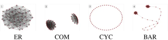
ER COM CYC BAR
Fig. 2. Four snapshots of the models used for the generation of the temporal network.
The simulated temporal network is generated using the follow-ing procedure: startfollow-ing from a graph without links, the algorithm adds or removes links at each time instant according to a probabil-ity depending on a prescribed graph. This probabilprobabil-ity is given in Table 2 and depends on whether an edge is in the prescribed graph and whether it exists in the graph at the previous instant. The algo-rithm runs during30 time steps for a prescribed graph. Four different graphs with a constant number of nodes equal ton = 49 have been used and drawn from the following models:
1. [0, 30] - Erd¨os-R´enyi model p = 0.5 (ER) 2. [30, 60] - Two cliques of variable size (COM) 3. [60, 90] - Cycle graph (CYC)
4. [90, 120] - Barbell model (BAR): two cliques of size 15 con-nected with a path of length19
These models represent three different structures which can be found in networks: random linkage of nodes in model 1, structure in communities in model 2 and regularity in model 3. Frequency patterns related to signals describing graphs with these structures have been highlighted in Fig. 1. The model 4 is a mixture between structure in communities and regularity.
4.2. Steps 1-2-3-4: Transformation into signals and identifica-tion of features with NMF
The graph at each time instant is transformed into a collection of signals and frequency analyses are performed to obtain the matrix V with the vectorized spectra at each time at each column. The NMF algorithm is applied to this matrix usingβ = 1, the number of features isQ = 3 and the number of iterations is 3000.
(a) Feature 1
(b) Feature 2
(c) Feature 3
Fig. 3. (left) Features found using NMF, reshaped in a matrix form to show magnitude of each frequency for each component. Con-nections can be made with magnitudes found in Fig. 1: feature 1 with (c), feature 2 with (b) and feature 3 with (a). (right) Levels of activation over time are displayed as well as the four intervals cor-responding to the four prescribed models used to build the temporal network.
Fig. 3 displays on the left the obtained features reshaped in a matrix form to show magnitude of each frequency for each compo-nent. Connections between frequency patterns highlighted in Fig. 1 and these features can be made. Feature 3 looks like the pattern of a Watts-Strogatz model of degreek = 2 (Fig. 1a) with high values on the diagonal. Feature 2 is close to the pattern of a graph with communities (Fig. 1b) where the magnitudes of low frequencies for the first components are very high. As for feature 1, the magnitudes spread out over all frequencies are related to those found for the Erd¨os-R´enyi model (Fig. 1c). These three structures correspond to the three models used to build the temporal network.
Levels of activation over time of features are displayed on the right of Fig. 3, as well as the four intervals corresponding to the four prescribed models used to build the temporal network. It reveals that the features are activated at the expected time steps. Feature 3 asso-ciated to a regular structure is fully activated when the model (CYC) is active, and activated with less intensity when the prescribed model is (BAR). For others time steps the feature is close to0. As to feature 2, linked with structure in communities, it is activated when models (COM) and (BAR) are actives, composed of cliques. Finally feature
1, corresponding to a random structure, is mainly activated when model (ER) is active and for model (COM), denoting the random structure inside communities which are not totally built as cliques. It is also activated at the beginning of each interval, describing the random transition between two prescribed graphs.
4.3. Steps 5-6-7: Transformation of features into static graphs
(a) Feature 1
(b) Feature 2 (c) Feature 3
W Fig. 4. Graphs built from features. (insert) Shape of the distribution of distances. The vertical line indicates the retained threshold. Ran-dom structure for feature 1, structure in communities for feature 2 and regular structure for feature 3 are visible.
Construction of subgraphs from features enables us to visualize the structure of the temporal network when the features are activated. Fig. 4 displays these subgraphs corresponding to the features. The layout takes into account the links between nodes and enables us to have an overview of the structure of these subgraphs. These struc-tures correspond to the frequency feastruc-tures by similarity with illus-trations given in Fig. 1. They also correspond to the models we used to build the graph. NMF is hence able to separate, in a temporal network with three different structures coupled between them, these subgraphs. This gives indication about their time instants of acti-vation. The shape of the distributions of weights used to build the subgraphs is displayed in insert in order to highlight the difficulty to choose a good threshold.
5. CONCLUSION
We have proposed a novel method to track the structure of temporal networks over time using NMF and duality between graphs and sig-nals. At each time, the temporal network is represented by a graph which is transformed into a collection of signals. NMF is used to discover features in the amplitude spectra of these signals; these fea-tures, whose levels of activation vary over time, represent a specific structure of the graph. The effectiveness of the method was demon-strated on a simulated temporal networks containing three types of structures.
These results provide insights in the characterization of tempo-ral networks, but also call for further studies, in particular concerning the parameters in the NMF in this context. The extension to a con-tinuous model for temporal networks, where some continuity in time of the transformation into signals, is also worth considering.
6. REFERENCES
[1] Mark Newman, Networks: An Introduction, Oxford University Press, Inc., New York, NY, USA, 2010.
[2] Petter Holme and Jari Saramki, “Temporal networks,” Physics
reports, vol. 519, no. 3, pp. 97125, 2012.
[3] Arnaud Casteigts, Paola Flocchini, Walter Quattrociocchi, and Nicola Santoro, “Time-varying graphs and dynamic networks,”
International Journal of Parallel, Emergent and Distributed Systems, vol. 27, no. 5, pp. 387408, 2012.
[4] Peter Grindrod and Mark Parsons, “Social networks: Evolving graphs with memory dependent edges,” Physica A: Statistical
Mechanics and its Applications, vol. 390, no. 21-22, pp. 3970– 3981, Oct. 2011.
[5] Andrea EF Clementi, Angelo Monti, Francesco Pasquale, and Riccardo Silvestri, “Information spreading in stationary markovian evolving graphs,” in Parallel & Distributed
Pro-cessing, 2009. IPDPS 2009. IEEE International Symposium on, 2009, p. 112.
[6] Kevin S. Xu, Mark Kliger, and Alfred O. Hero III, “Visualizing the temporal evolution of dynamic networks,” MLG’11, vol. 1, 2011.
[7] Andriana S. L. O. Campanharo, M. Irmak Sirer, R. Dean Malmgren, Fernando M. Ramos, and Luis A. N. Amaral, “Du-ality between time series and networks,” PloS one, vol. 6, no. 8, pp. e23378, 2011.
[8] Yuta Haraguchi, Yutaka Shimada, Tohru Ikeguchi, and Kazuyuki Aihara, “Transformation from complex networks to time series using classical multidimensional scaling,” in
Artifi-cial Neural Networks-ICANN 2009, p. 325334. Springer, 2009. [9] Yutaka Shimada, Tohru Ikeguchi, and Takaomi Shigehara, “From networks to time series,” Phys. Rev. Lett., vol. 109, no. 15, pp. 158701, Oct. 2012.
[10] Ronan Hamon, Pierre Borgnat, Patrick Flandrin, and C´eline Robardet, “Transformation de graphes dynamiques en signaux non stationnaires,” in Colloque GRETSI 2013, Brest, France, Sept. 2013, p. 251.
[11] Ronan Hamon, Pierre Borgnat, Patrick Flandrin, and C´eline Robardet, “Tracking of a dynamic graph using a signal theory approach : application to the study of a bike sharing system,” in ECCS’13, Barcelone, Espagne, Sept. 2013, p. 101. [12] Ronan Hamon, Pierre Borgnat, Patrick Flandrin, and C´eline
Robardet, “Networks as signals, with an application to bike sharing system,” in GlobalSIP 2013, Austin, Texas, USA, Dec. 2013, p. IPN.PB.8.
[13] Daniel D. Lee and H. Sebastian Seung, “Learning the parts of objects by non-negative matrix factorization,” Nature, vol. 401, no. 6755, pp. 788–791, Oct. 1999.
[14] Ingwer Borg and Patrick J.F. Groenen, Modern
multidimen-sional scaling: Theory and applications, Springer, 2005. [15] Hao Jianxiu, “Cyclic bandwidth sum of graphs,” Applied
Mathematics-A Journal of Chinese Universities, vol. 16, no. 2, pp. 115121, 2001.
[16] Ronan Hamon, C´eline Robardet, Pierre Borgnat, and Patrick Flandrin, “Relabeling nodes according to the structure of the graph,” Tech. Rep., Oct. 2013.
[17] C´edric F´evotte and J´erˆome Idier, “Algorithms for nonnegative matrix factorization with theβ-divergence,” Neural