An econometric analysis of the hog cycle in France in a simultaneaous cobweb framework and welfare implications

HAL Id: tel-02859555

https://hal.inrae.fr/tel-02859555

Submitted on 8 Jun 2020

HAL is a multi-disciplinary open access archive for the deposit and dissemination of sci-entific research documents, whether they are pub-lished or not. The documents may come from teaching and research institutions in France or abroad, or from public or private research centers.

L’archive ouverte pluridisciplinaire HAL, est destinée au dépôt et à la diffusion de documents scientifiques de niveau recherche, publiés ou non, émanant des établissements d’enseignement et de recherche français ou étrangers, des laboratoires publics ou privés.

Distributed under a Creative Commons Attribution - NonCommercial - NoDerivatives| 4.0 International License

implications

Louis Pascal Mahe, . University of Minnesota

To cite this version:

Louis Pascal Mahe, . University of Minnesota. An econometric analysis of the hog cycle in France in a simultaneaous cobweb framework and welfare implications. Economics and Finance. University of Minnesota, 1976. English. �tel-02859555�

An econometric

analysis

of

the

hog cycle

in

France 'in

a

simu]taneous cobweb framework

and

welfare

imp'l

ications

Louis-Pascal MAHE (1)

-

May 1976

-Dissertation

submitted

for

the

Ph.D. degree

at

the University

of

Minnesota

(1)

_I

want

to

thank many people who helped

ne

in

various

ways

during

this

research

:

Pr

L.

Martin

and M.

t{bel

who provided advices

at

various stages

i

research

fellows

at

the I.N.R.A.

and

the

finance

ninistry

with

whom

I

talked

several

times.

l4rs Leclainche deserves

particular

mention

for

having accepted

to

type a

manuscript

not

written in

her

mother langage

oocuueNTArtoH Éiot'toutg nuRA'e neHNes

t'Iou _{l"nou, these diagrons on uhieh}

uatiations

oùe"

tine of

pz'iees,

inte-rest

rates

ete...

aîe

rep?esented by upuards and douru'nrds

zig-zag

Lines.

I,lhile

I

uas annlysing

the

erises,

I

tried

seueraL times

to

ealeuLate these

peaks and tnotqhs by

_fittirq

irneguLaz'

euwes,

and

f

beLietse

tlnt

the

essen-tiaL

Laus

of

erises

eouLd be

matherna-tieally

determined on

the basis

of

such euroes.

I

stiLL

tlxL,nk

this

is

possibLe

gioen

suffieient

data"

..,

K.

MARX

l

i

I

TABLE OF

CONTENTS

INTRODUCT ION

Chap.

1

-

A SHORT REVIEW 0F LIVEST0CK CYCLES THEORY

1

-

Periodicity

2

-

Reversibility

and

the

nature

of

the supply function

3

-

The

relationships

between breeding

stock and supply

Chap.

2

-

INVENTORY-SUPPLY INTERACTION AND ITS

C0NSEQUENCES 0N THE SUPPLY FUNCTIoN

1

-

A supply

function

based on

inventory-sales interaction

2

-

Partial

adjustment and adaptive expectations

3

-

Supply

in

numbeis, supply

in

weights

4

-

Dynamics and

stability

conditions

5

-

Simul taneous

or

recursive

cobweb ?

Biases resul

t'ing

from unappropriate

estimation

procedure

Chap.

3

-

AN ECON0METRIC MODEL 0F THE HOG

SUBSECTOR IN FRANCE

L

-

General

setting

of

the

French hog

j _ndu

_stry

11

-

Production

1,2

-

Consumption, prices

i3

-

Trade, EEC and pol

icy

2

-

Data

available, implications for

specification

and

possible

biases

21

- The

supply block

22

-

Denand block 23

-

Trade equation

3

-

Empirical

results

3i

-

Compl

ete

model

32

-

Prel iminary work on supply 33

-

Structural

changes and supp'ly

el a stic i

ti

es Pages 1 14 14 4 6 B 10 2T 23 25 29 4t 41 41 51 5B 62 63 66 69 70 7L 89 96

Chap.

4

-

WTLFARE ANALYSIS 0F THE HOG CYCLE IN FRANCE

1

-

tlelfare loss

in

a

simple cobweb

2

-

Distribution

effects

3

-

l,lelfare

effects

of

fluctuations

.

in

a

more general model

3L

-

Consumers'surp'lus and marketing margins behavior

1

-

constant margins

2

-

proportional

margins

3

-

non

reversibility of retail

price fluctuations

32

-

A

first

appl

ication

to

the

hog

market Conclusion Appendix 4. CONCLUSION

*

x,É

99 99 101 104 104 104 105 107 108 LT7 1 2 3 4 4 t20 t22 124 130

Figure

2.1

-Figure

2.2

-Figure

3.1

-Figure

3.2

-Figure

3.3

-Figure

3.4

-LIST OF

FIGURES

Cobweb

with current price effect

Specif

ication

b'ias from assuming mi stakenly

a

recursive

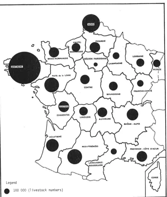
cobweb

Concentration

of

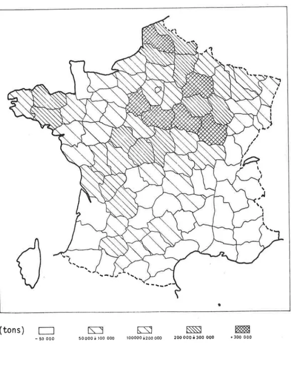
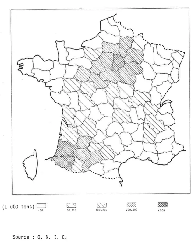
hog farming enterprises Map

of

feed

grains production

in

1974

a)

Barl ey

b)

Corn

Location

of

hog

production

in

France (1974)

Variation

of

consumption

per

head

for

various

kinds

of

meat (1963-1973)

Retail

meat

price

index

for

main meats

( 1e60-1e74)

Price

of

pork

_at

retail,

of

hogs

at

farm

level

and feeder

pigs

price

"Marketed" production and consumption

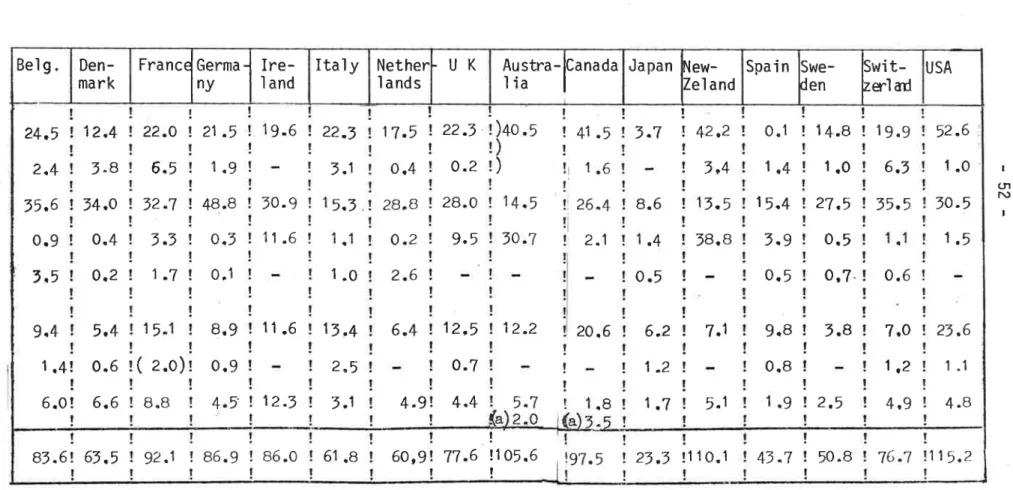
Relative

shares

of

countries

in

pork imports

(te74)

Beef and

veal

retail

price

indices Margin behavior

Actual

fitted

value,

supply

Actual

and

fitted

values

:

feeder pigs

price

Actual

and

fitted

values

:

demand

Actual

and

fitted

values

:

farm

retail

relation

Actual

and

fitted

values

:

net

imports

Cross-cornel ogram

Unconstra'i ned regression

pages 26 34 45 49 50 48 53 54 56 57 59 68 B5 87 87 BB 8B B9 91 91 Figure Fi gure Fi gure Fi gure Fi gure Fi gure Figure Fi gure Figure Fi gure Fi gure Fi gure Fi gure

3.5

-3.6

-3.7

-3.8

-3.9

-3.10

-3.11

-

3.n-3.13 - 3.14- 3.15- 3.163.I7 -I

Fi gu re Figure Fi gu re Fi gure Fi gure F 1 gure Fi gure Figure Fi gure Fi gure Fi gure Fi gure Fi gure Fi gure Fi gure Fi gure

3.18-

Constrained regression

3.19-

Correlogram

4.1

-

Symmetrical

stationary

cobweb

4.2

-

Distribution

effects

4.3

-

Constant margins and consumers'surplus

4.4

-

Proportionnal margins

4.5

-

Non

reversibjlity of

retail

prices

4.6

-

Surplus

deviations

in

the

comp'lete model

4,7

-

Implîcation

of

current price

effect

on we'lfare

4.8

-

Slow adjustment and

welfare

effects

4

.9'

-

Constant margins and

welfare

'losses

4.9 -

Equilibrium

path

S,

production

4.10

-

Equilibrium

_Rath

D,

consumption

4.11

-

Equilibrium

path

P,

farm

price

4.LZ

-

Equilibrium

path

Pi

retail

price

4.13

-

Producers'surplus-vagiation

as

%

of

equi-I

ibriurn

receipt

(P1.Q1) x 91 93 100 103 105 106 107

trz

t20 t22 124 L25 126 r27 t28 L29

lr

)r

LIST

OF

TABLTS

Table

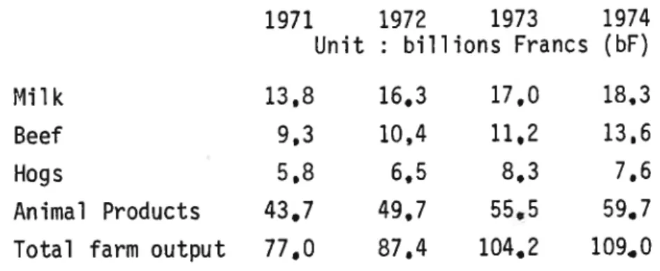
3.1

-

Importance

of

hog production

in

the

gross

farm output

Table

3.2

-

Size

distribution

and concentration

of

feeder pigs units

Table

3.3

-

Size

distribution

and concentration

of

slaughter

hogs

units

Table

3.4

-

Evolution

of

the

share

of

production

accor-ding

to

special

ized

hog operation

Table

3.5

-

Meat consumption

in

0CDE countries

Table

3.6

-

Relative

share

of

various meat product in

the

consumer

food

budget

Table

3.7

-

Some items

of

the

trade

balance

for

French agricul ture

Table

3.8

-

Total

pork meat produced

in

EEC countries

Table

3.9

-

Self

sufficiency rate

in

EEC countries

for

pork

Table

3.10-

Break down

of

the

production according to

the

type

of

buyer

Table

3.li-

Marketed supply

elasticities

Tabl

e

3.12

-

Some publ i shed estimates

of

supp'ly el

asticity

for

hogs

with

respect

to

hog

price

Table

3.13-

Demand

elasticities

Table

3.14-

Change

in

demand

elasticities

Table

3.15-

Short

run

marketed supply

elasticities

estimates o1

for

various specifications

Table

4.1

- Time

series

of

surp'lus deviations

)* pages BO B1 83 94 42 43 44 46 52 53 58 60 60 62 79

x)t

i19

So much has been

written about'livestock cycle

theory

that

it

seems

bold

to

try

again

bringing

some new

light

on

the subiect.

This

was

however

the

first

intention

of

my

dissertation.

Two

points

appeared

to

me

as deserving more

attention.

First

no economic model

of

livestock

supply

has

ever

included

a

demographical

part

expressed by

a

dynamic complete

model

in

the

line of

human popu'lations. Since

I

had studied

the

properties

of

such

a

model

Ijntented

to

analyse hog supp'ly

in

these

terms'

by

p'lug-ging

in

control

variables

related

to

supply behavior

of

hog producers.

This

turned

out

to

be unfeasible

for

lack

of

detailed

data

on inventories

of

hogs on

farm

in

France, which were necessary

to

set

up

the

model

in

a

demographjc framework. The

only data

available

over

a

long

enough period

of

time,

concern slaughtered hogs.

I

had

therefore

to

give

up

this

approach,

which would have

led

also

to

some

partjcular

estimation problems.

The second

point

I

wanted

to

study

in

a

systematic manner, was

the implications

of

the relationship

between

inventories

and slaughtered hogs

at

each

point

i.n time,

arelationship

which comes up natura'l'ly when the demographic approach

is

used.

Contrarily

to

my

first

impression

I

found out

that

this

was

not

really

a

new

idea.

Some authors and

particularly

Fox

ttil

and

Reutlinger

_[39],

have already analysed some aspects

of this

problem

in

the context

of

a

formalized mode'|.

Given

this

sjtuation,

the contribution

I

hopedto make on a more

general and moderately

theoretical

nature was

very

s'lim,

and an

alternatjve

focus

of

my

thesis

was

to

ana'lyse

the pecularities

of

the

hog

cycle

in

France and

to

put the stress

on

the estimation

of

the

underlying

relationshiPs,

â

work which had never been done

in

an econometric framevrork before

in

this

country.

-2-The

fina'l

output

of

my research

is

half-way between these

two

objectives.

In

the

first

chapter

I

discuss

the

two

well

known theories

of

livestock

cycles

namely

the

cobweb and

the

harmonic motion model, a'long

with the

published

formulation

of

the

inventory-supp'ly

interaction.

In

chapter

two,

I

attempt

to

clarify

the relationships

between

the

various

types

of

supply

specifications

used

in

hog models,

in

particular

between

recursive

and simultaneous

specifications

and between models exp'laining

first

inventories

on farms and those

:

explaining

directly

1 iveweight mar-keted by'lagged

price.

This

analysis

throws some new

light,

I

believe,

on

the

economic

interpretatjon

of

the

parameters estimated and essentia'l1y

the

supply

elasticity.

The

next

step

is

to

formulate

explicitely

the consequences

of

the

inventory-supply

interaction

on

the

dynamics

of

the

cobweb and

the

stability

conditions.

The

third

aspect

of

this

addition

to

the

cobweb

theory

is

the analysis

of

its

implications

on

estimation

pro-cedures, and an

analytical

discussion

of

the

biases which may

arise

in

both

supply

and

demand when recursiveness

is

unproper'ly assumed.

Chapter

three gives

an account

of

the

empirical results

of

estimation

on

the

basis

of

French hog

industry.

A'lthough

a

complete market model was

estimated, including

demand, margîns,

piglet

market, and imports,

emphasis has been

put

on

the

supply and

the other

equations have

not

re-ceived so much

attention.

Some

particular

features

of

the

French hog

jndus-try

and economic behavior

are

discussed

in

the

light of

these empirical

resu I ts .

Chapter

four

deals

with

an attempt

to

analyse

the welfare

as-pects

of

cyc'lica1

fluctuations.

The approach

is

based on surpluses and

follows the

line of

welfare

analyses

of

random

fluctuatjons

of

agricultu-ral

prices.

An

empirical

i'llustration

is

presented on

the

basis

of

the

estimated model

of

chapter

three.

It

allows

to

give

an

order

of

magnitude

of

the efficiency loss

due

to

the fluctuations

along

with the

resulting

djstribution

effects

both

in

the short

run

and

in

the

long

run.

This

last

chapter

is

one

of

the

possib'le

app'lications

of

the

estimated model which makes use

of

the theoretical

discussion

of

specification

problems. Since

-3-concept

of

surplus used must be

consistent

with

micro-economic foundations,

it

is

necessary

to

discuss

the

nature

of

the

supp'ly we are dealing with

before using

it

for

we'lfare analysis.

)r

x)Ê

-4-Chap.

1

-

A SH0RT REVITW 0F LIVESTOCK CYCLTS THEORY

Basically

two chemes have been proposed

_to

explajn livestock

cycles

:

the

cobweb and

the

harmonic motion. The cobweb theorem has

re-ceived considerable

attention

from

agricultura'l

economists, both from

a theoretical

and an

emp'irical

point

of

view.

Following

Lorie

_[31],

Larson _[ZA] fras

recently

argued

that

"The cobweb mode'l seems

to

be so

intrjgu'ing,

and so persuasive,

that

it

is

uncritically

accepted on meager

grounds". Then he goes

on

"there

is

a

basical'ly

different

model,

wich

i

have

termed harmonic motion

that

provides

a

more

likely

explanation

of

the

hog

cycle

and many

other

agricultural

production cyc1es".

In a

review

article

on both

theories

Mc Clements

_t34

criticises

Larson's

assertion

that

the superiority

of this

model is based on two main

issues

:

the periodicity

of

the

c.vcle and

the

reversibility of

the

supply

functions.

I

shall

review

the

discussion

of

these problems and

follow

with

the

estimation

procedure

difficulties.

But

first

Iet

us present

brief'ly

the

two model s.

Cobweb

vs.

harrnonic motion

In

his classical

article

on

the

cobweb theorem,

Ezekiel

_fg,

p.

272_l

states

three conditions

for

the theory

to

be

relevant

to

a

commodity

(i)

where production

is

completely determined by

the

producers'response to

price,

under

conditions

of

pure competition (where producer bases plans

for

future

production on

the

assumption present

prices

wi'11

continue,

and

that

his

own production plans

will

not

affect

the market)

;

(2)

where

pro-duction

cannotbeûranged,once plans are made

;

and

(3)

where

the

price is

set

by

the

supp'ly avai I abl e .

COBhIEB MODEL

(1.1)

demand

p

t

(

1.2)

supply _a;

=6+b

=C+dP

,b<0

at

t-t^l (1.3)

equilibrium

qi

= Qt

where rrr

is

the

time duration

of

the

production process. As

is

well

known,

this

model

yields

a

cycle

with

period

2

w,

and which

is

convergent

or

di-vergent according

to

the

relative

slopes

of

the

supply and

the

demand.

Ezekiel was aware

of

the limitations

of

such a model

to

explain

agricultu-ral

cycles.

He discussed

brief'ly the

possibility of

a

non

zero

short-run

elasticity

of

supply and mentionned

lag

of

farmers'

response

to

prices

which

could

increase w

in

the

above

specification.

Harmonic motion

differs

from

the

cobweb

in

the

behavioral as-sumption

with

regard

to

producers

:

"Reference

to

a

supply curve might well be supp'lanted by

a

decision

rube vrhich is

higly

conservative,

in

the

sense

of

involving

little

explicit

pnediction

of

future

events.

Producers do not

in

fact

decide

to

produce

a

given

level

of

output

in

response

to

an expected

price,

but

rather

decide

to

change

the current rate

of

production

jn

res-ponse

to

current prices,

or

current'level

of profits"

_[29'p.

169].

HARMONIC MOTION P

t

=ô-b

,d>0

at

( 1

.4)

demand (

1.5)

producers'behavior

dBt=c(p*-P)

dr

Qi*

_*

=

*

Br

(1.6)

production 'lag

-6-(1.7)

c'learing

where Ba

is

the

breeding

stock

and

F

is

the

equilibrium

price.

This model

generates

a

cycles

of

production and

prices

of

4 w.

1

-

Periodici

'The

chief

difficulty

in

accepting

tle

cobweb as

the

explanation

of

the

Hog cyc'le has been

that

the

hog cyc'le

is

usual'ly about

four

years

long

(s1ight1y

less

in

some

countries),

whereas,

in

view

of

the

i2

months

production

period

for

market

lveight

hogs,

the

cycle

should according to

the

cobweb theorern be two

years'long"

_Qg,

p.

l7?-1.

It

is

a

fact

that

known hog

cycles

have

a

period

of

more than two

years,

although one year

is

the

average production 1ag

(1).

fne

period

is

about

4 years

in

the

United

States, but

it

varies

from 36

to

40 months

in

most European countries ans

is

52 months

in

the

Netherlands _[ZO,

p.144].

This

evidence g'ives support

to

l.arson's assertion

that

his

model is

consistent

with the

facts,

and he

considers

that

the

arguments advanced

to

reconcile

the

cobweb

with

observed

periodicity

are

not

very

convincing

;

they are

based mostly on

a

1ag

bet-ween

prices

and oroduction response

_{flS, p. 34.}

l'lcClernents suggested mistakenly

that

Nerlove's

partial

adiustment

hypothesis

is

one way

to

a1ter the period.

"Depending on

the

speed

of

adjust-ment

this

model can imply

cycles

of

more than

twice

the

production 1ag" _f32,

p.

145].

It

is

clear

however

in

Nerlove's

artic'le

_[SO,p.n[,

that

neither adaptive expectations

nor

partial

adjustment hypothesis

alters

the

periodi-c'ity

s'ince

the difference

equation

of

prices

andquantities

is

still of

order

one.

0n1y

the

stabi'lity

domain

is

en'larged due

to

the

fact

that

the

producers'

short

run

reaction

is

less

than

the

long run

supp'ly

elasticity

would imp1y.

(1)

Technical progress has reduced

the

production

lag,

and

it is

now

approa-ching

10 months.

llle cannot

therefore

do away

with

the

assumption

of

a

response 1ag'longer than

the

nroduction 1ag

if

the

cobweb

is

to

be

the

framework used

to

exnlain

the

hog cycle.

Is

there

however

a great

difference

between

the

economics

invol-ved

in this

hypothesis and

the

one underlying

the

mathematical formulatjon

of

Larson ? There should be an

intuitive

explanation,

based on economic

analysis

or

technology,

of

the

fact

that

the

phase angle between price

and production

is

trvice

the

production 1ag. Larson does

not give

such an

explanation,

hesays on1y,

"First

there

is

a

shift of

90 degrees

(i.e.

one

fourth

of

the

period)

cause by

price

being equa'l

to

the rate

of

change

of

planned

output,

and then

there

is

a

further

shift

of

90 degrees caused by

the

fixed

production

1ag"

_Pg,p.

379].

The

solution

of

the

differentjal

equation derived from model

(1.4)

to

(1.7)

given by Larson

_[tS,p.fZe]

is

(assuming bcm

₌

1), (1.8) (1.e) p1 ₌ coS

(+

*

.p)

e1 = coS

(+

*

.q)

(ii)

p1 ₌

coS

_*

"Where,'if

eO and eO

differ

by

n

radians,

the

solutions

are

consistent

and

the

system is

in

resonance".

But equations

(1.8)

and

(1.9)

solved

explicitely

with

respect

to

time,

have

built

in

an

implicite

relationship

between g1 and pt_Zw.

Taking

_.p

_{= 0}

and e.,

=

'rT

r

as

naquired by Larson

for

resonnance we

get

(1)

nt

(i)

Q1 =

cos

(

m

*n)

(1)

There

is a lot of

od.dness

in the

assumptions on

the coefficients

which

-B-From

(i'i)

pt_z*

= cos

_{# tt}

-

2w)

Pr-zu,=cosf*-tl

compared

to

(i)'it

implies

(1)

'Qt

₌

pt-zu,.This relationships

comes from

the

reduced form

of

(1.4)

and

(1.5),

but

the lag

connot

orig'inate

in

the demand where adjustment

is

instantaneous.

It

must

therefore

be

built

in

the

"supp'ly"

equation,

which supposes,

quite

similarly

to

what cobvreb users

do,

that

there

is

a lag

between

price

changes and response tothem. l{oreover

the

constraint

making resDonse

lag

equal

to

the

production 1ag

is

quite

strong.

The main

objection

to

Larson's model

is

that

the

underlying econo-mic

theory

is

unclear.

His model may

well

represent

reality,

but

it

does

not

explain

why

the

periodicity

is

4

times production 1ag. The

superiority

of

harrnonic motion over

the

cobweb

is

open

to

question,

at

least

on the

periodicity

point

of

view,

to

which Larson

gives great tleight.

2

-

Reversibil it.y and

the nature

of

the

supply function

Ezekiel's

exposition

of

the

cobweb theorem has been

criticized'

ma'in1y on

the

basis

of

the

reversibility

of

the

supp'ly curve

involved

_[1'

6].

It

is

clear

that

the

domain

of

application

of

the

cobweb

is

in

the explanat'ion

of

short

run

fluctuatjons.

However

the

revers'ibility

implied

in

the

treatment

of

the theory

is

a

long-run

characteristic.

From

this

observation,

Ackerman suggests

that

producers'behavior

js

_better

expressed by

sh'ifts

of

the short

run

normal supp'ly

curves.

"Bet-ween

the

sharply

rising

market supply curve and

the very

s'low1y

rising

long

term

supply

curve, there

exists,

accordinglY,

for

some time fol'low'ing

cultivation

year

a moderately

rising

short

term normal supp'ly

curve"

L1'

p.15a].

This

would lead

to

a

cobweb converging more

easily

than assumed

This point

js

certainly

valid, for

it

is

always

a

delicate

task

to

inter-pret

supply

elasticity

estimates

in

the

light of

static

supply

theory

and consequently

for

po]icy

purposes. The

partial

adiust-ment arguadiust-ment and Johnson'sfixed

asset

theoryp{

gPaiong

withthis

I

ine

of

interpretation.

But

this is

more

a

prob'lem

in

supply

theory

than

in

cobweb

theory.

And what

it

changes

in

the

latter is

mainly

the

stabjlity

condi-tions.

In

any case,

while

the

supply curve has an economic basjs

re-lated

to

the

equilibrjum

of

the

firm

and

of

the industry,

it

is

not

so

for

Larson's equation

(1.5).

The economic

interpretation

of

the

coeffi-cient

c

in

(1.5)

for

example

is

not cJear.

Furthermore'an estimation

procedure has

not

been developed

for

the structural

equations

of

the model

(1.4)

to

(1.7).

Empirical

verifications

put

forth

by Larson [Ze]' French and

Bressler

(1) or others

partman,16]

are

based

only

on

the

pe-riodicity

argument usjng

spectral

analysis

or

similar

techniques-

This is

a rather

roundabout method

of

empirical verification.

In

the specification

of

equation

(1.5) there

is

an interest'ing

point

made by Larson,

especially

for

the livestock

cycles

he

actually

had

jn

_mind.

_It

js

the

assumption

that

breeding decisions

are

made contjnuous'ly

over

time.

But

there

exists a constraint

on decisions

at

any po'int

in

time

which

is

not

taken

into

account.

Altering the

breeding

stock

81 cannot be

achieved

without'influenc'ing

the

sales

of

females

for

slaughter

at

time

t

because

the

stock

of

animals

in

the

whole herd

at

t

is

fixed

by past

dec'i-sjons.

Therefore

sales

Q

at

t

do

not

depend

only

on

the

breeding stock

at

t -

w

like

in

equation

(1.6)

but also

on

the

change

in

B

at

the

same

time

t. If

this

has

ljttle

relevance

to

crops

for

which seeds count

for

a

very

small

fraction

of

the output,

it

is

a

genuine

part

of

livestock

product.ion and

its

consequences should

therefore

be

explored.

tr'Je shall

do

this

within the

cobweb

theory

where

it

is

simpler as

far

as

interpre-tatjon

and

estimation are

concerned.. We

wilI

see

that

if

this

biologica]

(1)

_Considered by Larson "most dramatic

verification of the

model". The

-10-constraint

is

accounted

for,

modification

of

the

supp'ly equation

is

requi-red

with

an

interpretation

of

supply parameters going along

with

it.

A

ne-gatively

sloping

short run

supp'ly response

follows,

which changes the

dynamics

of

the

cobweb and

the

stabjlity

condjtions.

A

practical

conse-quence

of

this

point

of

view

is

that

the

model

loses

its

recursiveness and simultaneous equations

are

then

required

throughout.

3

-

The

relationships

between breeding stock and supply

Supply

theory

deals

with the

relation

between

output

prices

and

quantjties

(1)

produced. However some students

of

hog supply use

far-rowings as dependent

variable

_[tS]

while others

use

quantities

marketed

measured through

slaughter

_ll,

26).

As data on farrow'ings and

invento-rjes

are

not available

in

many

countries

jncluding

France, we may

raise

the question

of

the relationships

between

the

two

specifjcations.To

be more

spec'ific,one may wonder

if

the

supply

elasticity

derived from

the

two

specificatjons

has

the

same meaning.

This

can be done by

trying

to

find

out

the

analytical

correspondence between

the

supply

specified

as

a

lagged

prices

marketed

quantities

relationshjpontheonehand, and supply specified

as

a

lagged

prices

-

inventories (or

farrowings)

relationship,

on the

other

hand.

The second

point

to

explore

is

the rationale

and

the

consequences

of

the relationships

between changes

in

supplies

and

in

the

breeding

stock-Conceptual'ly

thjs

i

s not a

new

idea.

Ezekiel

has al ready mentionned possi b1e

short

run

adiustment

of

the

supply,

and Breimyer

_[S,

p.

Z]

gave an

explic'it

justificatjon

of

the

necessity

to

study breeding

stock

and supply changes

jointly

:

"When

prices

of cattle

are

high,

producers

hold

back stock

for

(1)

And more

generally, of

course,

with factor prices

and even

prices of

breeding. The supply

of

cattle

for

slaughter:

is

reduced and

prices

are

puÉhed

still

higher.

Inventory

of cattle

build up.

As progeny

of

jncreased

numbers

of

breeding

stock

reach slaughter age annual slaughter

starts

upward. Eventuelly

it

increases

a

lot,

and

it

reduces

prices

to

a

point

that

djscourages

further

expansion

of

production and,

later,

results

jn 1

iquidation

of

inventorjes".

A new

step

was made by Reutl

inger

_[Ag] who gave

the

first

for-mulation

of

the

ideas expressed by Breimyer. He introduced

the

notion

of

demand

for

cow

inventories

which

is

mostly

influenced by

output

prices,

and showed

that

prices

lagged one

year

have

a

negative

effect

on cow

slaughter.

But he

did

not carry

the

argument

far

enough

to

formulate the

implications

on

stability,

specificatjons

bias

and

estimation. This

may

be

the

reason why Hayenga and Hacklander

]1,

p.

54{

were unable

to

use

this

ljne of

analysis

to

explain

their

hog supply

findings

wh'ich exhibited

a

negative

short-run price

elasticity

:

"This

rather

stong

negative

sup-p1y response

is

quite

intrigu'ing,

since

it

differs

from

the

response by

cattle

feeders".

Even more

intriguing

is

the positive short

run

response

for cattle, in

the

light of

later

results.

Tryfos

_{l+4 is}

the

first

to

have

translated Reutlinger's

model

into

the

simultaneous equations framework

in

a

systematic manner

(1).

He

found evidence supporting

the

jnfluence

of

inventory

variations

on the

suppljes

of

beef,

vea1, mutton and

pork.

The model may be summarized as

fol

I ow.

A

biological

dynam'ic

relationship,

(

1.10)

A,

= an

+

at

lt_t

(1)

Dean and Heady

_[el

and Fox

_[tt]

had found

a small

instantaneous

price

effect

on

the supply.

But they

did not

separate

the

two components of

short-run

suppty

;

change

in

numbers, and change

in

average

weight.

More-ver, they

found opposite signs

for the current price effect. It is

also

quite surprising that neither Reutlinger nor Tryfos refer to Hildreth

and

Jarret's

book where

a formulation of the inventory

supply

interaction is

explicitely given

and

in a

form

very close to equation (1.13)

betow _[-19,

where :

(1.11)

with:

(1.12)

-L?-A,

is

the

quantity

of

livestock

avai'lable

at

t

It-t

is

the

inventory

at

the

beginning

of

the

period Desired I

ivestock

inventorY'

0

+b

1 b2

P, current price

of

meat,

bt

>

C,

current price

of

feed,

bt

<

Pt*

b

ri

ct

Parti

a'l

adiustment hYPothesi s

'

0 0

Ir

-

Ir-1

=

.

(IT

-

It-r)

,0<c<1

Tota'l

supply equation,

(1.13) St=At-d (Ir- It-l)

where

d

is expected

to

be c'lose

to

one.

.

',Thus

the

mode'l

calls

for

the

simultaneous

estimation

of

the

following

system

of

equations

:"

(1.14) It =.

bo

+

c

bt

Pt

+

c

b,

Ct

*

(1

-

c)

It-t

(1.15)

Sr

= u0

+ (at

+ d)

-dI

1

t

Empirical

results

confirmed

the

expected

signs

of

the

functions

i.e.

positive

effect

of

price

on

current

inventory

and negative

effect

of

curyent inventories

on

current

supply.

Tryfos'model

is

quite similar

to I

_t

Reutlinger,s

specification

;

the

simultaneity

in

Tryfosrcase comes from making

desired inventory

depend on

current price

instead

of

price

la9-ged by one

period

as

in

Reutl'inger's model .

l^lhile

the

idea

of

inventory

changes has been

clearly

expressed and

correctly

estimated in tlrepreviousmode'ls,

the interpretation

of

the

functions involved,

the

meaning

of

parameters

with

reference

to

the

supply

part

of

the

cobweb,

the

consequences

of

the specification

effor

made in

usfnga

recursive

mode1, and

the

imp'lications onthedynamicsofthe cobweb have

not

been

clearly

stated.

This

is

what

I

would

like

to

show and

il-lustrate

on

the

basis

of

the

hog industrSr

in

France'

x

-14-chap.

2

-

INVENToRY-SUPPLY INTERACTI0N AND ITS CoNSEQUENCES 0N THE SUPPLY FUNCTION

In

this

chapter

I will

develop a model

of

hog supply along the

line of

Reutlinger and Tr3rfos,

but

I will

set

it

in

the

cobweb framework'

so

that

the interpretation

of

the

various

specifications

used becomes

easier.

I will

also

show

that

this

model, where supply depends on current

prjce

and

price

lagged by w

units

of

time

(w

=

production

lag),

takes a sinrple autoregressive form when

partial

adiustment

or

adapt'ive expectations

are

assumed. The long

run

supp'ly

elasticity

may

then

be derived

in

a

s'irnple

way

as

in

other

llerlove's

type

models.

This

specification

is

part'icu1ar1y

useful

when

little

aggregation

is

made over

time

e'g'

when

quarterly

data

are

used.

The

current price

affects

both numbers and we'ights

of

anjmal s

slaughtered

at

each

point

in

time.

The

relation

between

specification

jn

numbers and

live

weight

js

also

discussed'

Then,

I

analyse

jn

a

formalized way

the

consequences

of

the

current

pr.ice

effect

on

the

dynamics

of

the

cobweb and

the

estimation

pro-bl ems.

i -

A suppl.y

function

based on j nventor.y-

sales

interaction

Both Reut'linger and

Tryfos

sfrecified a

model

with a

high level

of

aggregation over

time

by

using

annual

data.

I

use

a

model where the

define

the state

of

the

herd by

a vector

Xa.whose components

are

the

num-bers

of

individuals

jn

each

properly

defined age and physiolog'ical classes.

Then

there

is

a

dynamic

relationshio

between

the state

vectors

at

succes-sive points

in

tjme, name'lY,

(2.r)

Where

the matrix

M, 'includes both demographic parameters

(ferti-lity,

survival

rates

₎

and

control variables

corresponding

to

farmers

deci sions.

Now

if

we

can't

use

this

detailed

framework because

of

incom-plete data,

we may

still

consider

the

dynamical

relationship

between some

components

of

the state vector.

Consider

the

age group

of

individual s which may be

either

bred

or

sold

for

slaughter

at

time

t,

its

number de-pends on

the

number

of

females bred w

unjts

of

time before.

Then ure may

write

(1),

(2.2) H

t

=mB

t-w

xt

=

Mt

xt-i

Where, H

is

total

number

of

individuals

(herd)

ready

to

be bred

or

slau-ghtered

at

t.

This

corresponds

to

the

'lavailable

supply" of

Reutl ï nger

is

the

number

of

females bred

at

time

t-w.

It

corresponds

ap-prox'imate'ly

to

the

jnventory

demand

of

Reutlinger

(Breeding

stock).

is

a technical coefficient characteristic

of

the

species,

for

hogs

it

lies

between 5 and 10 (saved

pig'lets

per

litter).

t

B t-w

1) I do not

use

Reutlinger-Tryfos notations since, partly

due

to the

smal-ler

time

unit, the definition of variables relates to

narrower groups

of

animals

in the specification I

use. m

-16-But

at

each

unit

of

time

we do have

a technical

identity

cons-traint

relating

cument

supply and

current

breeding

stock (inventory

demand).

(2.3)

where,

St

is

the

marketed supplyn

i.e.

the

sales

or

the

slaughtered

ani-mals (1).

This constraint

has been

stated

by Reutlinger

with Bt

-

Bt-t

instead

of

the

level

of

B,

but

forgotten

about by several authors

subse-quent'l

v

G).

Tryfos

relaxed

this

constraint

in

(1.14)

,

which seems

iusti-fied

only

by

the

high leve'l

of

aggregation over

time

(annua'l

data)

and

over types

of

animals.

Equations

(2.3)

and

(2.2)

show

that

available supply'in

pre-determined

at

time

t,

by previous decisions made on

Bt_*.

However marketed

supply

is

not

fixed,

since decisions made

at

t

on BX

will

also

affect

mar-keted

supply.

Let

us assume

for

the

moment immediate adiustment

to

current

price,

and

formulate

farmers'decisions.

cr,O

+

aP,

where

P,

is

basically

output

price,

but

may be generalised as

a vector

of

output

price, factor

prices, substitutesprices.

Equations

(2.4)

means

that

when producers

think that

their

operation

becomes more

profitable

they are

ready

to

increase

their

ouptut,

and

for

doing so

they

increase

their

pro-duction

capacity

Br.

(2.4)

may

then

be thought

of

as

a

factor

demand

equa-(1)

When

there are various

types

of

animals

sold for

meat

in a

species

like

beef, a vector identity

would

sinplify Reutlinger's

formulation.

(2) In particular, it is susprising that

Larson, whose model has some

simu-larities to Reutlinger's

one, and should include

naturally the constraint

(2.3), did not

discuss

this question in his

1967

article.

+

Ht=

Bt

st

Bt=

tion

where

output

price

plays the

maior

role

(1).

Combining

(2.4)

and

(2.2)

we

get

what should be considered in my

opinion as

the true

supply equation

in

livestock

models.

(2.5)

Ht mcr' + moP,-"

This

is

the relationship

between

the

avai'lab1e supply

at

t

and

the

lagged

price

which has

actually

induced

this

livel

of

supp'ly,

or

more

rigorously

this

level

of

production.

As

the

concept

of

supply

elast'ic'ity

refers

to

the

relative

variation

of

output

induced by

price variation,

whether

this

output

is

sold

or

stocked by

the

fjrms,

the relevant

parameter

to

evaluate supply

elasticity

should be m

o.

Becuase

of

the

linear

form the supply

elasticity

should be estimated

at

mean values

by

:

(2.6)

o

= ITl0 _:-P

H

This

is

the

procedure used by Harlow

_[tS,

_R.

39],

whose model explained

the

farrowings

by lagged

price.

Available

supply

is

_iust

m tjmes

the

farrowings and both models

yie'ld the

same

e1asticity

as

far

as

spec'i-f

ication

is

concerned

(practica'l

prob'lems may lead

to

d'ifferences).

However,

several workers used marketed supply

St

as

the

dependent

variable,

because

it

js

the

only available data [Kettunen,

26

_].

Combining

(2.3),

(2.4) and

(2.5)

we

get

the

marketed supply equation :

Sr=Hr-Bt

St

=

*o0

*

*oPt_*

-

c*g - oPt

(1)

Since

Bt

may be both

sold

and

invested,

output

price influencing factor

demand

is actually

expected

price tl, oppottunity cost is actually

Pa

which should

affect

Ba

negatively. Sorting out the

two

effects is

a

rather frustrating task

as shown by Myers

et al. in a slightly different

context, dealing with

average

_{weight Ea,}

35].

(2.7)

(2 .B)

-18-St

=

o0

(m-1) + moPr-*

-

*Pt,

which we may

write,

St

= a0 *

tlPt_"

*

n'Pt,

t1

t 0,

n0

.

0

Then one can see

that while

it

is

correct

to

assume

recursive-ness

in

Harlow's speci'Fication

(2.5),

jt

is

no

longer

thecasewhen the explained

variable

is

the

number

of

hogs marketed.

This

has obviously

estimation consequences which

will

be taken up

later

on

But suppose also

that

(2.8)

were

correctly

estimated

with

respect

to

n1,

i.e.

that

plim

ô1 =

m

o

One would

calculate the

supply

elastic'ity

by,

(2.e) P

= mCÈ=

S o1

Internal

consistency

of

the

model

implies

H

>

5,

and therefore

the

supply

elasticity is

overvalued by

ol

t

o.

This

is

actually

what some

of

the

results

of

Kettunen show when he used successivel.v

available

supply

and marketed supply as

the

dependent

variable

_126,

p.

481. The

price

elas-ticity

of

marketed supply was

0,25,

while the

result

with the "quantity

of

pork produced" as dependent

variable

was

0,20.

The

difference

(1)

is

not

big,

but

Kettunen quotes

results

of

an author who found 0,40

for

marketed supply

elasticity.

There may be

other

pecu'larities

which

also

contribute

to

explain the

difference.

I

do

not

know

of

any American study which would

allow

to

verify

th'is

comparison between

o,

and

o.

The above evidence does

not

appear as

a

dramatic

verification

of

the analysis.

However, we can see

on

a

priori

basis

that

the

approx'imation

of

oby

o,

is

not

really

far

away.

The

relationsh'ips

on mean values may

help

to

evaluate

the

discrepancy.

H=B+S

F=mE

B=S/m-1

m

m-T

S

(1)

The

difference

seems even

smaller in

view

of the

use

of a recursive

mo-del,

which

implies further overestimation,

as

will

be seem

later.

H

which

implies

the

relation

between

o,

and o

g.1

6

Hm

S

m-1

Therefore

if

m

is

close

to

5

for

hogs,

the

error

is

25 %,

which

is non

inconsistent

with

Kettunen

resutts

(1).

0f

course

if

data

on inventories are

available,

which

is

a

great

estimation

advantage as

will

be seem

later'

one can

explain

the

marketed sypply by

current price

and lagged breeding

stock,

as done by some

authors.

Combining (2.2)

,

(2.3)

and

(2.4)

gives

(2.10)

St

= m Bt-u, -

cr'

-

cr, P,

In Tryfos'notations,

assuming fu11 adjustment

(c

=

1,

and

d =

1),

the single

equation on marketed supply

is

written

as

(2.11)

St

= â0

*

(at

+

1)

It-t

-

b0

-

blPt

-

bzCt

These equat'ions

(2.10)

and

(2.1L)

make cl ear why

current

price

effect

should be negative when marketed supply

is

explained by lagged

inven-tories

and

current

price.

Fai'ling

to

take

the

inventory-supp'ly

interaction

has

led

some workers

to

find their

results surprising

as already noted

lZO,

p.

50

;

L7

;27; 35

].Now,

how

to

derive

the

supply

elasticity

from

(2.10)

and

(2.1I)

?

One

could

get

the

rirarketed-supply

elasticity

ot

defined

bV

(2.9)

by

estimating

(2.10).

(2.10)

has

the

disadvantage

of

adding

a

non

linearity

to

get the

product mo. But as

will

be

seen'later (2.8)

leads

to

estimation

djfficulties

due

to

the

corre'lation

between

Pr-*

and Pa.

Apparent'ly

Tryfos

did

not

see

the

a

priori

relationship

bet-ween

the

coefficient

of

lagged

inventory

a1 and

the

cument

price

ef-(1)

rf

_one

_defines

o0

=

-of,,.r,

approxima.t;t't.ot

î:.t".;":n:t

elasticitv

is

given

by

ot

+ oO since

m

o,i -ob = 5

tm

-

1)

= mcr6 = o

-20-fect

b,(1).

I

think

this

has

led

him

to

give

improper

definitions

to

the

I

elasticities

derived

from

the

two simultaneous equations

(1.i5)

and (1.16) which becomes when

d

₌

c

=

1r

(1. 15' ) b1 bzct

(1.16')

St

₌ a0

+

(at

+

1)

It-t -

11

He

called

inventory

e'lasticity

the

parameter derived from

(1.15'),

while

this

is

the true

supply

elasticity, in

the

usual

definition

of

supply.

(1.15')

is

the

equivalent

of

(2.4)

which would

give the

elas-ticity

expressed as,

For,

if

we assume again F = mE

from

(2.2),

then

(2.6)

becomes :

ir=bo+

Pt*

6 ott = 0! B P

o

= lll

0;

H

PP

=ma*=0i=O"

mBB

0n

the

other

hand he

cal'led

supply

elasticity

the

negative

short

run

effect

derived from both

the

equations, presumably

the

expres-sion

db,

_{! .}

But,

althrough

it

affects current

supply,

this

parameter

is

in fact

ràt.t.a

to

inventory

demand and shou'ld be

interpreted

as

such and

certainly not

as

something

like

short run

supply.

What

I

consider

to

be

a

misleading

interpretation

of

the

para-meters

of

the

estimated equations on

a

supply

point

of

view,

may be seen

again

in

the

Reutlinger

-

Tryfos'models. Although

they both

introduced a

partia'l

adjustment hypothesis

in

their

mode'l

they

did not

try

to

derive

long run

elasticity

of

supply from

their

results,

which

they rea1ly

were

(1)

Probably because

of

the

way he

speclfied

in

0,1,4')

the

marketed supply

as

the difference

between

available

supply

A,

and change

in

inventories

in

a position

to

do. But,

assjmi'lating

current price

effect

to

short

run supply response prevented them

to

think

of

the

inventory

ecluations

(2.4),

(2.5)

or

(1.15)

as

true

supp'ly

functions,

with

both

short

and long run aspects when

the introduction

of

partial

adjustment

or

adaptive

expecta-tions give

them an autoregressive form.

2

-

Partial

adj ustment and adaPt

ive

expectations

Since decisions

are basically

made on breeding

stock

it

is

natural

to

define the

"slow adjustment"

at this'level.

The behavioral equation

(2.4)

becomes now,

(2.12) oo +

partial

adiustment hypothesis means,

(2.13)

Bt

-

Bt_1

=

I

(tT

-

tr-r)

,

o.< 1r<

1

adaptive expectations imp1y,

OPT

Bi

(?.r4)

(Pi

-

PT_r) =

o

(Pt

-

PT_l)

,0<û-<1

As

urell

known when

either

one

of

the

two assumptions

is

intro-duced

alone

(e.g.

_ç

+

L, û = 1) the

estimab'le equation takes

the

same form.

If

both

are

introduced,

then one cannot

identifycp

and rp. Assuming Û

=

1'

we

get the

equation expressed

in

observable variab'les,

(2.15)

Br =1o0

+

(1

-

f)

Br-1 +

_?oPr

Again,

in

Tryfos'case

the coefficient

of

Pt

(in

1.15

as

in

15)

is

what

js

usually ca'lled

short

run

e'lasticity

when

multiplied

by

E

.

The

long run

elastjcity

is

obtained by

dividing byct.

The equation

.15)

may

easily

be expressed

in

terms

of

available

supply

or

production,

2.

p/

-22-H,

= mBr-* gives

(2.16)

Ha = mtgo' + m

(1

-

?)

Bt_*_l

+ mgaPr_*

This 'is

an

unpractical

equation

to

estimate, but the

marketed supply equation

is

much

nicer

to

both estimate and

interpret.

By using

(2.15)

and

(2.t6)

St Hr Bt

St

=

goo

(m

-

1)

+

(1

- q)

(tBt-,u-l

-

Bt-t)

+ mfoPg-y

-

_loPt

Using

the

relation

between Hr_, and

Bt-*_l

we

get the

simp'le autoregressive marketed supply equation,

(2.t7)

S,

=

1o6

(m

-

1)

+

(1

-

.f)

St-l *

mgaPr-"

-

,foPt

This

equation

includes

both

partial

adiustment and

inventory-supp'ly'interaction

in

a

form

close

to

the

cobweb.

In

this

equation mga

will

serve

to

calculate short

run

supp'ly

elasticity,

mo'long

run

supply

e]asti-city,

qo the

inventory

demand

effect.

But

it

should be noted

that

using 5

instead

of

H means, as

said

before,

that

this

procedure

overstates

supply

elasticities

and

yields

the marketed supply

elasticities

(SR and LR).

Equation

(2.17)

takes an

interesting form, since,

although

it

involves

price

lagged by w

units

of

time, the introduction

of

a

partial

ad-justment _assumption

_is

_made by

using

the

dependent

variable

lagged by

just

one

unit

of

time.

This

would

not

be abvious

if

one

specifies

supply behav'ior

directly

on

a

marketed supply equation

of

the

form

Sf

₌

f

(Pt-*)

jn

the

recursive

case.

It

is

then tempting

to

specify

partial

adiustment

with

the

production 1ag w as

a

unit

of

thime as,

sr S

(si

-

st_*)

t-w

=9'

which would

lead

to

an estirnable equation

St

=

f'

(St_w, Pt_.W

where

the

coefficienf

of

Sa-,

would be

interpreted

as one minus the

adjustment

coefficient

q'.

At

one

time

I

made such an

attempt,

without any success. Kettunen had

also

done

the

same

_{V6, p.}

51], but the

coef-fjcient

was

very

snall

(0,08)

and

not

significant.

The simple form given

to

the

marketed supply equation

with

slow adiustment by

the

breed'ing stock-supply

jnteraction

seems

to

add

a nice

coherence

to

the

averall

supply behavior

implied

by

the

model. The

results turn out

to

be

accepta-ble

for

the

lagged nrarketed supply, ôS we

shall

see

later

on.

3

-

Supplv

in

numbers, supplv

in

weiqhts

All

the

previous models have been

specified

in

numbers. But

the

relevant

variable

on market

equilibrium

is

the

IiVeweight

marketed.

Current

prices

have

a positive

effect

on average carcass we'ights, as well known,

ê.g.

Harlow

_[15,

p.

40].

More

recently,

Myers, Havliceck and

Hen-derson

_[34

,

35

_]

have provided us

with

a

more sophisticated model

of

short run

(1)

supply behavior.

Basically,

they

consider

the

problem

of

theprofitabilityofdelaying

the sales

of

fattened

animals when

prices

are

changing. They expect

total

'live

weight

at

time

t

to

depend

positively

on

current price

and

negatively

on

the

pnice expected

for

the next

unit

of

time,

where

the available

animals

at

t will still

be

in

the

suitable

weight range

for

slaughter.

The

difficulty is

that

expected

prices

depend

heavily

on

current prices,

as

the

authors were avare

of,

making impossible

to

separate

the

two

effects.

It

seems

to

me

that

they could have

intro-duced

in

their

model one more

function

based on

the

relationship

between

hogs'age and

their

average

weight

;

they could

have then

sorted

out

the

(1)

Compared

to the

previous

short run elasticity this

problem".