Uncertain Logical Gates in Possibilistic Networks. An Application to Human Geography

(1)

HAL Id: hal-01203515

https://hal.inria.fr/hal-01203515

Submitted on 23 Sep 2015

HAL is a multi-disciplinary open access

archive for the deposit and dissemination of

sci-entific research documents, whether they are

pub-lished or not. The documents may come from

teaching and research institutions in France or

abroad, or from public or private research centers.

L’archive ouverte pluridisciplinaire HAL, est

destinée au dépôt et à la diffusion de documents

scientifiques de niveau recherche, publiés ou non,

émanant des établissements d’enseignement et de

recherche français ou étrangers, des laboratoires

publics ou privés.

Uncertain Logical Gates in Possibilistic Networks. An

Application to Human Geography

Didier Dubois, Giovanni Fusco, Henri Prade, Andrea G. B. Tettamanzi

To cite this version:

Didier Dubois, Giovanni Fusco, Henri Prade, Andrea G. B. Tettamanzi. Uncertain Logical Gates in

Possibilistic Networks. An Application to Human Geography. Scalable Uncertainty Management, Sep

2015, Québec, QC, Canada. pp.249-263, �10.1007/978-3-319-23540-0_17�. �hal-01203515�

(2)

Uncertain Logical Gates in Possibilistic Networks.

An Application to Human Geography

Didier Dubois1_{, Giovanni Fusco}2_{, Henri Prade}1_{, and Andrea Tettamanzi}3

1

IRIT – CNRS, 118, route de Narbonne, Toulouse, France

2

Univ. Nice Sophia Antipolis/CNRS, ESPACE, UMR7300, Nice, France

3

Univ. Nice Sophia Antipolis/CNRS, I3S, UMR7271, Sophia Antipolis, France dubois@irit.fr, fusco@unice.fr, prade@irit.fr,

andrea.tettamanzi@unice.fr

Abstract. Possibilistic networks offer a qualitative approach for modeling epis-temic uncertainty. Their practical implementation requires the specification of conditional possibility tables, as in the case of Bayesian networks for probabil-ities. This paper presents the possibilistic counterparts of the noisy probabilistic connectives (and, or, max, min, . . . ). Their interest is illustrated on an example taken from a human geography modeling problem. The difference of behaviors in some cases of some possibilistic connectives, with respect to their probabilistic analogs, is discussed in details.

1 Introduction

Bayesian networks [11] can be built in two ways: statistical and subjective. In the first case, a supposedly large dataset involving a number of variables is available, and the Bayesian network is obtained by some machine learning procedure. The probability tables thus obtained have a frequentist flavor, and the simplest network possible is searched for. On the contrary, Bayesian networks can be specified using expert knowl-edge. In this case, the structure of a network relating the variables is first given, often relying on causal connections between variables and conditional independence rela-tions the expert is aware of. Then probability tables must be filled by the expert. They consist, for each variable in the network, of conditional probabilities for that variable, conditioned on each configuration of its parent variables. Note that, even if causal rela-tions as perceived by the expert are instrumental in building a simple and interpretable network, the joint probability distribution obtained by combining the probability tables no longer accounts for causality. Another difficulty arises for causality-based Bayes networks: if variables are not binary and/or the number of parent variables is more than two, the task of eliciting numerical probability tables becomes tedious, if not im-possible to fulfill. Indeed, the number of probability values to be supplied increases exponentially with the number of parent variables.

To alleviate the elicitation task, the notion of noisy logical gate (or connective) has been introduced, based on the assumption of independent causal influences that can be combined. As a result, one small conditional probability table is elicited per parent variable, and the probability table of each variable given its parents is obtained by com-bining these small tables by a so-called noisy connective [6, 10], which may include a

(3)

so-called leakage factor summarizing the causal effect of variables not explicitly present in the network.

While the notion of noisy connective solves the combinatorial problem of collecting many probability values to a large extent, the issue remains that people cannot always provide precise probability assessments. Let alone the fact that the probability scale is too fine-grained for human perception of belief or frequencies, some conditional prob-ability values may be ill-known or plainly unknown to the experts. The usual Bayesian recommendation in the latter case is to use uniform distributions, but it is well-known that these do not properly model ignorance. Alternatively, one may use imprecise prob-ability networks (called credal networks) [12], qualitative Bayesian networks [14] or possibilistic networks [3]. While the two first options extend probabilistic networks to ill-known parameters (with an interval-based approach for the former and an ordinal approach for the latter), possibilistic networks represent a more drastic departure from probabilistic networks. In their qualitative version, possibilistic networks can be de-fined on a finite chain of possibility values and do not refer to numerical values. This feature may make the collection of expert information on conditional tables easier than requiring precise numbers obeying the laws of probability.

In this paper, we propose possibilistic counterparts of noisy connectives of prob-abilistic networks. As possibilistic uncertainty is merely epistemic and due to a lack of information, we shall speak of uncertain connectives. After recalling probabilistic networks with noisy gates, we present the corresponding approach for possibilistic net-works and present various uncertain gates, especially the AND, OR, MAX, and MIN functions.4Finally, the approach, including algorithmic issues, is illustrated on a belief network stemming from an application to human geography.

2 Probabilistic Networks with Independent Causal Influences

Consider a set of independent variables X1, . . . , Xnthat influence the value of a

vari-able Y . In the ideal case, there is a deterministic function f such that Y = f (X1, X2, . . . , Xn). In order to account for uncertainty, one may assume the

existence of intermediary variables Z1, . . . , Zn, such that Ziexpresses the fact that Xi

will have a causal influence on Y , and to what extent (Zi has the same domain as Y ).

It is assumed that the relation between Xi and Zi is probabilistic and that Xi is

in-dependent of other variables given Zi. Besides, we consider the deterministic function

as affected by the auxiliary variables Zi only. In other words, we get a probabilistic

network such that

P (Y, Z1, . . . , Zn, X1, X2, . . . , Xn) = P (Y, Z1, . . . , Zn) · n Y i=1 P (Zi| Xi), (1) 4

The idea of possibilistic uncertain gates was first considered empirically by [13] directly in the setting of possibilistic logic, at a time where possibilistic networks had not yet been in-troduced. It seems that the question of possibilistic uncertain gates has not been reconsidered ever since, if we except a recent study in the broader setting of imprecise probabilities [1] and a preliminary outline in French by the authors [4].

(4)

where P (Y, Z1, . . . , Zn) = 1 if Y = f (Z1, Z2, . . . , Zn) and 0 otherwise. This is

called a noisy function. In particular, notice that the dependence tables between Y and X1, . . . , Xn can now be obtained by combining simple conditional probability

distri-butions pertaining to single factors:

P (y | x1, . . . , xn) = X z1,...,zn:y=f (z1,...,zn) n Y i=1 P (zi| xi). (2)

This is the assumption of independence of causal influence (ICI) [6]. In the case of Boolean variables, it is assumed that P (zi = 0 | xi = 0) = 1 (no cause, no effect),

while P (zi = 0 | xi = 1) can be positive (the effect may or may not appear when the

cause is present).

Canonical ICI models are obtained by means of specific choice of the function f . For instance, if all variables are Boolean, f will be a logical connective. In this case, we speak of noisy OR (f = ∨), noisy AND (f = ∧); if the range of the Zi’s and Y is a

totally ordered set, usual gates are the noisy MAX (f = max), or MIN (f = min). The approach may be further refined by allowing f to summarize the potential ef-fect of external variables not taken into account: this is the leaky model. Now, Y also depends on a leak variable Z`not explicitly related to specifically identified causes, i.e.,

Y = f (Z1, Z2, . . . , Zn, Z`). The domain of Z`is supposed to be the range of f , i.e.,

the domain of Y and this variable is independent of the other ones. Hence, the leakage model may be written as:

P (Y, Z1, . . . , Zn, Z`, X1, . . . , Xn) = P (Y, Z1, . . . , Zn) · P (Z`) · n Y i=1 P (Zi| Xi), so that P (y | x1, . . . , xn) = X z1,...,zn,z`:y=f (z1,...,zn,z`) P (z`) · n Y i=1 P (zi| xi). (3)

For instance, in the case of Boolean variables, P (y = 1 | x1= 0, . . . , xn= 0) may be

positive due to such external causes.

We will now turn to the question whether the same kind of ICI approach can be used to elicit possibilistic networks as well.

3 Canonical Possibilistic Networks

Possibility theory [7, 16] is based on maxitive set functions associated to possibil-ity distributions. Formally, given a universe of discourse U , a possibilpossibil-ity distribution π : U → [0, 1] pertains to a variable X ranging on U and represents the available (incomplete) information about the more or less possible values of X, assumed to be single-valued. Thus, π(u) = 0 means that X = u is impossible. The consistency of information is expressed by the normalization of π : ∃u ∈ U, π(u) = 1, namely, at least one value is fully possible for X. Distinct values u and u0may be simultaneously

(5)

possible at degree 1. A state of complete ignorance is represented by the distribution π?(u) = 1, ∀u ∈ U . A possibility measure of an event A ⊆ U is defined by

Π(A) = sup

u∈A

π(u). Possibility measures are maxitive, i.e.,

∀A, ∀B, Π(A ∪ B) = max(Π(A), Π(B)).

The underlying assumption is that the agent focuses on most plausible values, neglect-ing other ones. A dual measure of necessity N (A) = 1 − Π(U \ A) expresses the certainty of event A as the impossibility of non-A.

A possibilistic network [2, 3] has the same structure as a Bayesian network. The joint possibility for n variables linked by an acyclic directed graph is defined by

π(x1, . . . , xn) = ∗i=1,...,nπ(xi| pa(Xi)),

where xiis an instantiation of the variable Xi, and pa(Xi) an instantiation of the parent

variables of Xi. The operation ∗ is the minimum (in the qualitative case) or the product

(in the numerical case).

Deterministic models Y = f (X1, . . . , Xn) are defined as in the probabilistic case:

π(y | x1, . . . , xn) =

(

1 if y = f (x1, . . . xn);

0 otherwise. (4)

Let us define possibilistic models with independent causal influences (ICI). We use a deterministic function Y = f (Z1, . . . , Zn) with n intermediary causal variables Zi, as

for the probabilistic models. Now, π(y | x1, . . . , xn) is of the form:

π(y | z1, . . . , zn) ∗ π(z1, . . . , zn| x1, . . . , xn),

where π(y | z1, . . . , zn) obeys Equation 4. Again, each variable Zi only depends (in

an uncertain way) on the variable Xi. Thus, we have π(z1, . . . , zn | x1, . . . , xn) =

∗i=1,...,nπ(zi| xi). This leads to the equality

π(y | x1, . . . , xn) = max z1,...,zn:y=f (z1,...,zn)

∗i=1,...,nπ(zi| xi), (5)

whose similarity with Eq. 2 is striking. Notice that, when ∗ = min, Eq. 5 boils down to applying the extension principle [16] to function f , assuming fuzzy-valued inputs F1, . . . , Fn, where the membership function of Fiis defined by µFi(zi) = π(zi| xi).

In case we suppose that y depends also in an uncertain way on other causes sum-marized by a leak variable Z`, then the counterpart of Eq. 3 reads:

π(y | x1, . . . , xn) = max

z1,...,zn,z`:y=f (z1,...,zn,z`)

∗i=1,...,nπ(zi| xi) ∗ π(z`). (6)

In the following, we provide a detailed analysis of possibilistic counterparts of noisy gates.

(6)

3.1 Uncertain OR and AND Gates

The variables are assumed to be Boolean (i.e., Y = y or ¬y, etc.). The uncertain OR (counterpart of the probabilistic “noisy OR”) assumes that Xi = xi for at least one

variable Xirepresents a sufficient cause for getting Y = y, and Zi = ziindicates that

Xi = xi has caused Y = y. This gives f (Z1, . . . , Zn) = W n

i=1Zi. The uncertainty

indicates that the causes may fail to produce their effects. Zi = ¬zi indicates that

Xi = xi did not cause Y = y due to the presence of some inhibitor that prevents the

effect from taking place. We assume it is more possible that Xi = xicauses Y = y

than the opposite (otherwise one could not say that Xi = xiis sufficient for causing

Y = y). Then we must define π(zi | xi) = 1 and π(¬zi | xi) = κi < 1. Besides,

π(zi | ¬xi) = 0, since when Xi is absent, it does not cause y. Hence the causal

elementary possibility table:

π(Zi|Xi) xi¬xi

zi 1 0

¬zi κi 1

Note that in the case of a probabilistic network, π(zi | xi) is replaced by 1 − κi in

the above table. We can then obtain the table of the conditional possibility distribution π(Y | X1, . . . , Xn) by means of Eq. 5:

π(y | X1, . . . , Xn) = max z1,...,zn:z1∨···∨zn=1

∗ni=1π(zi | Xi)

=maxn

i=1 π(zi| Xi) ∗ (∗j6=imax(π(zj | Xj)π(¬zj | Xj));

π(¬y | X1, . . . , Xn) = max z1,...,zn:z1∨···∨zn=0

∗n

i=1π(zi | Xi)

= π(¬z1| X1) ∗ · · · ∗ π(¬zn| Xn).

Let us denote by x a configuration of (X1, . . . , Xn), and let I+(x) = {i : Xi = xi}

and I−(x) = {i : Xi= ¬xi}. Then we get:

– π(¬y | x) = ∗i=1,...,nπ(¬zi| Xi= xi) = ∗i∈I+(x)κi;

– π(y | x) = 1 when x 6= (¬x1, . . . , ¬xn);

– π(¬y | ¬x1, . . . , ¬xn) = 1, π(y | ¬x1, . . . , ¬xn) = 0: ¬y (no effect) can be

obtained for sure only if all the causes are absent. For n = 2, this gives the conditional tables:

π(y | X1X2) x1¬x1 x2 1 1 ¬x2 1 0 π(¬y | X1X2) x1 ¬x1 x2 κ1∗ κ2 κ2 ¬x2 κ1 1

More generally, if there are n causes, we have to provide the values of n parameters κi.

For the uncertain OR with leak, we now assume that f (Z1, . . . , Zn) = Wn_i=1Zi∨

Z`, where Z` is an unknown external cause. We assign π(z`) = κ` < 1 considering

that z`is not a usual cause. We thus obtain

– π(¬y | x) = ∗i=1,...,nπ(¬zi| Xi= xi) ∗ π(¬z`) = ∗i∈I+(x)κi;

– π(y | x) = 1, if x 6= (¬x1, . . . , ¬xn);

(7)

– π(y | ¬x1, . . . , ¬xn) = κ`(even if the causes xiare absent, there is still a

possi-bility for having Y = y, namely if the external cause is present). Indeed, we get (letting ¬x = ¬x1, . . . , ¬xn),

π(y | ¬x1, . . . , ¬xn) = max(π(y | ¬x, z`) ∗ π(z`), π(y | ¬x, ¬z`) ∗ π(¬z`)))

= max(1 ∗ κ`, 0 ∗ 1) = κ`.

For n = 2, the conditional table becomes:

π(y | X1X2) x1¬x1 x2 1 1 ¬x2 1 κ` π(¬y | X1X2) x1 ¬x1 x2 κ1∗ κ2 κ2 ¬x2 κ1 1

The only 0 entry has been replaced by the leakage coefficient. For n causes, we have now to provide the values of n + 1 parameters κi.

The uncertain AND (counterpart of the probabilistic “noisy AND”) uses the same local conditional tables but it assumes that Xi = xi represents a necessary cause for

Y = y. We again build the conditional possibility table π(Y | X1, . . . , Xn) by means

of Eq. 5 with f (Z1, . . . , Zn) =V n

i=1Zi. Thus, we find

– π(¬y | x1, . . . , xn) = maxz1,...,zn:¬y=z1∧···∧zn∗

n

i=1π(zi| xi) = maxni=1π(¬zi |

xi) = maxni=1κi;

– π(y | x1, . . . , xn) = 1;

– π(¬y | x) = 1, π(y | x) = 0 if x 6= (x1, . . . , xn) (if at least one of the causes is

absent, the effect is necessarily absent). For n = 2, Eq. 5 yields the conditional tables:

π(y | X1X2) x1¬x1 x2 1 0 ¬x2 0 0 π(¬y | X1X2) x1 ¬x1 x2 max(κ1, κ2) 1 ¬x2 1 1

More generally, if there are n causes, we have to assess n values for the parameters κi. The case of the uncertain AND with leak corresponds to the possibility π(zL) =

κL < 1 that an external factor ZL = zLcauses Y = y independently of the values of

the Xi. Namely f (Z1, . . . , Zn, ZL) = (Vn_i=1Zi) ∨ ZL. For n = 2, Eq. 5 then gives the

conditional tables: π(y | X1X2) x1 ¬x1 x2 1 κL ¬x2 κL κL π(¬y | X1X2) x1 ¬x1 x2 max(κ1, κ2) 1 ¬x2 1 1

3.2 Comparison with Probabilistic Gates

It is interesting to compare the possibilistic and probabilistic tables. Consider those of the noisy OR [6], where κi= P (¬zi| xi):

P (y | X1X2) x1 ¬x1 x2 1 − κ1κ21 − κ2 ¬x2 1 − κ1 0 P (¬y | X1X2) x1 ¬x1 x2 κ1κ2 κ2 ¬x2 κ1 1

(8)

There is an important difference between the behaviors of uncertain and noisy OR if ∗ = min. In the possibilistic tables, we see (using the associated necessity measure N , and Boolean notations for the instantiations of x1and x2) that N (y | 11) = max(N (y |

10), N (y | 01)) while P (y | 11) > max(P (y | 10), P (y | 01)), so that the presence of two causes does not reinforce the certainty of the effect wrt the presence of the most influential cause. Hence qualitative possibility networks will be less expressive than probabilistic networks. If ∗ = product, N (y | 11) = 1 − κ1κ2 > max(N (y |

10), N (y | 01)) as with the probability case.

Another major difference will occur in case the effects of causes are not frequent, as when P (¬zi | xi) = κi > 0.5, i = 1, 2. Then it may happen that P (y | x1x2) =

1 − κ1κ2> 0.5, that is the presence of the two causes makes the effect frequent. Then a

possibilistic rendering of this case must be such that π(¬zi| xi) = 1 > π(zi| xi) = λi

(say). However, there is no way of observing this reversal effect, since π(y | x1x2) =

max(λ1 ∗ λ2, λ1, λ2) = max(λ1, λ2) < 1. Hence π(¬y | x1x2) = 1 and N (y |

x1x2) = 0. In other words, using the uncertain OR, two causes that are individually

insufficient to make an effect plausible are still insufficient to make it plausible if joined together. Note that this fact reminds of the property of closure under conjunction for necessity measures in possibility theory (N (y1) > 0 and N (y2) > 0 imply N (y1∧

y2) > 0) which fail to hold in probability theory.

and π(y | x2) < π(¬y | x2), which is perfectly compatible with possibility theory. We

will outline a solution of this kind in the next section for the uncertain MAX, which is a generalization of the uncertain OR. However, one cannot build the global table from the marginal ones using an uncertain OR.

3.3 Uncertain MAX and MIN Gates

The uncertain MAX is a multiple-valued extension of the uncertain OR, where the output variable (hence the variables Zi) is valued on a finite, totally ordered, severity

or intensity scale L = {0 < 1 < · · · < m}. We assume that Y = max(Z1, . . . , Zn).

Zi = zi ∈ L represents the fact that Xi alone has increased the value of Y at level

zi. The conditional possibility distributions π(y | xi) are supposed to be given. We can

then compute the conditional tables, as π(y | x1, . . . , xn) = max z1,...,zn:y=max(z1,...,zn) ∗n i=1π(zi| xi) =maxn i=1 π(Zi= y | xi) ∗ (∗j6=iΠ(Zj≤ y | xj)) .

In a causal setting, we assume that y = 0 is a normal state, and y > 0 is more or less abnormal, y = m being fully abnormal. Suppose that the domain of Xiis L as well. It

is natural to assume that:

– if Xi= j then Zi= j, which means Π(Zi= j | Xi= j) = 1;

– Π(Zi> j | Xi= j) = 0 (a cause having a weak intensity cannot induce an effect

(9)

– 0 < Π(Zi < j | Xi = j) < 1 (a cause having strong intensity may sometimes

only induce an effect with weak severity, or may even have no effect at all); – An effect with severity weaker than the intensity of a cause is all the less plausible

as the effect is weak. This leads to suppose the following inequalities:

0 < π(Zi= 0 | Xi= j) < π(Zi= 1 | Xi= j) < · · · < π(Zi= j | Xi= j) = 1.

This leads to state the left-hand side table below (for 3 levels of strength 0, 1, 2).

π(Zi| Xi) Xi= 2 Xi= 1 Xi= 0 Zi= 2 1 0 0 Zi= 1 κ12i 1 0 Zi= 0 κ02i κ01i 1 π(Zi| Xi) Xi= 2 Xi= 0 Zi= 2 1 0 Zi= 1 κ12i 0 Zi= 0 κ02i 1 where 0 < κ02

i < κ12i < 1, 0 < κ01i < 1. In case we have m levels of strength, we have

to assess m(m+1)₂ coefficients. On the right-hand side is the corresponding table when the variables Xiare Boolean (then the middle column is dropped).

The global conditional possibility tables are thus obtained by applying Eq. 5, using the values of π(Zi| Xi), as given in the above table.

π(Y = j|x) =maxn

i=1 π(Zi= j|xi) ∗ (∗`6=iΠ(Z`≤ j|x`)).

For n = 2, m = 2, when the Xi’s are three-valued and Boolean, respectively, the

following conditional tables are obtained (in the Boolean case, only 4 lines remain):

x π(2 | x) π(1 | x) π(0 | x) (2, 2) 1 max(κ12 1 , κ122 ) κ021 ∗ κ022 (2, 1) 1 1 κ02₁ ∗ κ01 2 (2, 0) 1 κ12 1 κ021 (1, 2) 1 1 κ01₁ ∗ κ02 2 (1, 1) 0 1 κ01 1 ∗ κ012 (1, 0) 0 1 κ01₁ (0, 2) 1 κ12 2 κ022 (0, 1) 0 1 κ01₂ (0, 0) 0 0 1 x π(2 | x) π(1 | x) π(0 | x) (2, 2) 1 max(κ12₁ , κ12₂ ) κ02₁ ∗ κ02 2 (2, 0) 1 κ12 1 κ021 (0, 2) 1 κ12₂ κ02₂ (0, 0) 0 0 1

More generally, If we have m levels of strength, and n causal variables, we need

nm(m+1)

2 coefficients for defining the uncertain MAX. If we take into account the leak,

we have to add m(m+1)₂ coefficients per variable, in order to replace the 0 by a leak co-efficient in the conditional tables π(Zi| Xi) (assuming that an effect of strong severity

may take place even if the causes present have a weak intensity).

As for the uncertain MAX wrt uncertain OR, the uncertain MIN is a multiple-valued extension of the uncertain AND, where variables are valued on a the intensity scale L = {0 < 1 < · · · < m}. We assume that Y = min(Z1, . . . , Zn). We can then

compute the conditional tables, as

π(y | x1, . . . , xn) = max

z1,...,zn:y=min(z1,...,zn)

∗n

i=1π(zi | xi)

=maxn

(10)

The conditional possibility tables are thus obtained by applying Eq. 5, using the same values of π(Zi| Xi), as in the case of the uncertain MAX. For n = 2, m = 2, this

gives the following conditional tables (for ternary and binary inputs, respectively):

x π(2|x) π(1|x) π(0|x) (2, 2) 1 max(κ12₁ , κ12₂ ) max(κ02₁ , κ02₂ ) (2, 1) 0 1 max(κ02 1 , κ012 ) (2, 0) 0 κ12₁ 1 (1, 2) 0 1 max(κ01 1 , κ022 ) (1, 1) 0 1 max(κ01₁ , κ01₂ ) (1, 0) 0 0 1 (0, 2) 0 κ12₂ 1 (0, 1) 0 0 1 (0, 0) 0 0 1 x π(2|x) π(1|x) π(0|x) (2, 2) 1 max(κ12 1 , κ122 ) max(κ021 , κ022 ) (2, 0) 0 κ12₁ 1 (0, 2) 0 κ12 2 1 (0, 0) 0 0 1

As observed in the previous section when comparing the uncertain OR to the noisy OR, the simultaneous presence of a number of causes, which, taken in isolation, do not normally produce an effect, may lead to a plausible effect under a noisy MAX, which can never be the case with an uncertain MAX. Yet situations of this kind do arise in applications and are fully compatible with possibility theory. In order to make the elici-tation of possibility tables describing such situations easy, an appropriate uncertain gate has to be designed, by providing a suitable uncertain function f which can trigger an effect through the accumulation of enough weak causes. One idea we have tested in or-der to approximate such behavior is the proposal of the uncertain MAX with thresholds, described in Section 4, which, in addition to the usual parameters of an uncertain MAX, takes a threshold θjfor each value yjof the effect variable Y (threshold gates also exist

in the probabilistic setting [6]). Such threshold is an integer expressing the minimum number of causes that have to concur in order for effect yjto become possible.

4 Implementation

A prototype involving the uncertain connectives defined above, allowing to execute possibilistic models such as the one described in Section 5 has been implemented in R. Here, we give some details about the practical implementation of the uncertain con-nectives defined in the paper. Due to space limitations, we focus in particular on the uncertain MAX (and its variant with thresholds), whose implementation is non-trivial.

The way the uncertain MAX is implemented is shown in Algorithm 1. The parame-ter prm taken as input by this algorithm may be thought of as representing a set of rules of the form

Xi1 = xi1∧ . . . ∧ Xim = xim⇒ Y ∼ (κ(y1), . . . , κ(yn)), (7)

where the Xij on the left-hand side are parent variables of Y in the possibilistic

graph-ical model, the xij are one of their values, and (κ1(y1), . . . , κ1(yn)) is a normalized

possibility distribution over the values of variable Y , i.e., for all y ∈ Y , κ(y) ∈ [0, 1], and maxy∈Y κ(y) = 1. Notice that this generalizes the uncertain gates to the case of

multivalued variables. The left-hand side of a rule may be empty (i.e., m = 0): in that case, the rule is interpreted as if it were

(11)

Algorithm 1UNCERTAIN-MAX(Y, prm).

Generate a conditional possibility table for variable Y given its causes X1, . . . , Xn

using the uncertain MAX with the given parameters prm.

Input: Y : the effect variable; prm = {hcondi, kii}: a set of normalized possibility distributions ki =

(κi1, . . . , κikY k), maxj=1,...,kY k{κij} = 1, which apply when condition condi holds; condi =

(hXij, xiji), a (possibly empty) array of pairs of a cause variable Xijand one of its values xij; condiholds if

Xij= xijholds for all j; an empty condition always holds.

Output: π(Y | X1, . . . , Xn): a conditional possibility distribution of Y given its causes X1, . . . , Xn.

1: π(Y |X1, . . . , Xn) ← 0

2: for all x ∈ X1× . . . × Xndo

3: K ← {k : hcondi, ki ∈ prm, x |= condi} {Select the parameters that apply to x}

4: for all y = (y1, . . . , ykKk) ∈ YkKkdo

5: β ← mini=1,...,kKk{κiyi}

6: y ← max¯ i=1,...,kKk{yi}

7: π(¯y | x) ← max{β, π(¯y | x)} 8: end for

9: end for

10: return π(Y | X1, . . . , Xn)

Such rules may be used to represent leak coefficients, which apply to all possible com-binations of causes.

The antecedents of the rules fed into the uncertain MAX must cover all possible combinations x ∈ X1× . . . × Xn of the values of the parent variables of Y in order

to ensure that the resulting conditional possibility distribution π(Y | X1, . . . , Xn) be

normalized. We may notice that, if a leak rule of the form of Eq. 8 is given, that rule alone already covers all combinations of parent variable values and is thus a sufficient condition for the normalization of π(Y | X1, . . . , Xn); in that case, the parameters of

the uncertain MAX may be underspecified.

The uncertain MAX with thresholds, whose implementation is shown in Algo-rithm 2, has an additional parameter, which consists of an array of thresholds (θ1, . . . , θkY k), with θi ∈ {1, 2, . . . , kX1× . . . × Xnk}. Each threshold is associated

with one value y of Y and represents the minimal number of combinations of the causes for which y is more possible than the baseline possibility given by the leak coefficients (κ(y) > κ`(y)), or zero if no leak is provided.

5 Application

The metropolitan area of Aix-Marseille in southern France has experienced ongoing social polarization since the 1980s. The geography of unemployment, on the one hand, and the concentration of high-skilled professionals, on the other, contribute consider-ably to the structuring of a contrasted metropolitan social morphology [5, 9]. Knowl-edge of factors inducing social polarization of the municipalities in the metropolitan area is nevertheless uncertain. Several factors contribute to the valorization or to the devalorization of the municipal residential space. But these factors have “soft”, uncer-tain impacts on the phenomena under investigation: the same causes can not always lead to the same effects. A probabilistic model of these socio-spatial mechanisms has already been proposed [15] (cf. Fig. 1) in the form of a Bayesian network (BN). The BN was built using expert knowledge elicited through noisy logical gates (OR, AND,

(12)

Algorithm 2UNCERTAIN-MAX-THRESHOLD(Y, prm, thr).

Generate a conditional possibility table for variable Y given its causes X1, . . . , Xn

using the uncertain MAX with thresholds with parameters prm and thresholds thr.

Input: Y : the effect variable; prm = {hcondi, kii}: a set of normalized possibility distributions ki =

(κi1, . . . , κikY k), maxj=1,...,kY k{κij} = 1, which apply when condition condi holds; condi =

(hXij, xiji), a (possibly empty) array of pairs of a cause variable Xijand one of its values xij; condiholds if

Xij = xijholds for all j; an empty condition always holds; thr = (θ1, . . . , θkY k): the minimal number of

combinations of values of the causes for which each value of Y is more possible than the leak. Output: π(Y | X1, . . . , Xn): a conditional possibility distribution of Y given its causes X1, . . . , Xn.

1: π(Y |X1, . . . , Xn) ← 0

2: κ`← 0

3: for all hcondi, ki ∈ prm : condi= > do

4: κ`← max{κ`, k}

5: end for

6: for all x ∈ X1× . . . × Xndo

7: cnt← 0 {A vector of counters, one for each y ∈ Y }

8: K ← {k : hcondi, ki ∈ prm, x |= condi} {Select the parameters that apply to x}

9: for all y = (y1, . . . , ykKk) ∈ YkKkdo

10: β ← mini=1,...,kKk{κiyi}

11: y ← max¯ i=1,...,kKk{yi} 12: if β > κ`(¯y) then 13: cnty¯← cnty¯+ 1 14: end if 15: if cnty¯≥ θy¯then 16: β ← 1 17: end if 18: π(¯y | x) ← max{β, π(¯y | x)} 19: end for 20: end for 21: return π(Y | X1, . . . , Xn)

and MAX). We thus developed a possibilistic network (PN) using uncertain logical gates (OR, AND, standard MAX, and MAX-threshold) in order to link the same 26 variables of the BN (there is only one (ternary) MAX-threshold, with 7 parents). The parametrization of the PN was made compatible with the BN parametrization using the “most prudent” probability-to-possibility preference-preserving transformation, i.e., the T₁−1converse transformation of [8], well suited to treating subjective probabilities, in order to transform probabilistic parameters into possibilistic ones.

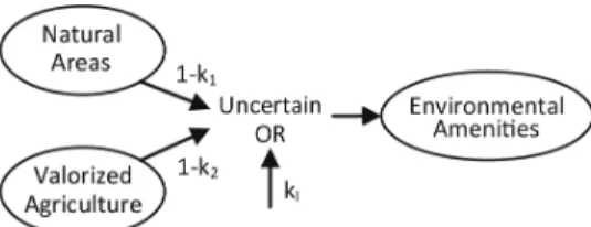
In Fig. 2 we show how an Uncertain OR logical gate can be used to generate a TPC. Only three parameters must be elicited: the possibilistic force of the two parent variables on the child variable (necessity of the consequence given that the parents are sufficient causes) and the leak parameter, which takes into account the activation of the consequence from secondary causes not included in the model. This table allows pos-sibilistic inference from uncertain knowledge. If, for example, for a given municipality of the study area, we are relatively certain of having natural areas (Π = 1, N = 0.5) and if it is only partially possible that we have valorized agricultural areas (Π = 0.5), we can infer that it is relatively certain (N = 0.5) that the municipality in question has environmental amenities.

Another difference with the probabilistic model is the possibility of keeping track of the ki parameters in the inference, in order to follow the sensitivity of results to

the parameters of uncertain causation. The advantage of uncertain logical gates can be better appreciated in the whole model (Fig. 1). Evolution is, for example, a ternary

(13)

Fig. 1. The BN model for the valorization/devalorization of municipalities in the study area (from [15]).

variable (having three values: no evolution, valorization, and devalorization) depending on 5 binary variables and a 4-value variable. The TPC is thus made of 3 × 25× 4 = 384 parameters, whereas the uncertain MAX-threshold gate used in our PN model only requires 27 parameters.

Both the BN and the PN model were thus used to produce trend scenarios for social polarization in the 439 municipalities of the Aix-Marseille metropolitan area. The future state variable that is inferred in these scenarios is the ternary variable Situation T2, having three possible values: Valorized (V ), Devalorized (D) or Other (O).

Both scenarios are based on uncertain knowledge of relationships among variables and produce uncertain evaluation of the future state of the metropolitan area in terms of social polarization. Nevertheless, the probabilistic model infers a most probable value of Situation T2for each municipality. This often gives a fallacious impression of certainty: probability differences between inferred values can be relatively small. The possibilis-tic model, using a min-max logic, produces in many cases sets of completely possible values (Π = 1). We thus decided to test the significance of the probability differences in the BN model: only probability differences exceeding a given threshold were consid-ered different. For a given threshold, we could thus infer even with the BN small sets of most probable values for some municipalities.

If no threshold is considered, the most probable values inferred by the BN and the completely possible values inferred by the PN coincide only in 54.7% of cases. In the remaining cases, possibilistic results are more uncertain and always include probabilis-tic results (most probable values are always completely possible for the PN).

The best agreement between the two models is obtained with thresholds 0.20 and 0.25 (lower and higher values give worse results). 72.4% and 77.2% of the inferred values are then identical. Most probable values are almost always compatible with PN solutions: they are included in the completely possible values as, for example, when {V, O} are the most probable values and {V, O, D} is the set of completely possible

(14)

Fig. 2. Generation of a TPC through an Uncertain OR logical gate.

values. The inverse is not always the case: depending on threshold value, 24% and 18% of possibilistic solutions are not included in the most probable values.

In conclusion, uncertain logical gates made the construction of the PN model possi-ble. The use of most probable solutions of the BN model often gives a false impression of certainty. In order to compare results from the BN and the PN models, we need to en-large the notion of most probable values: solutions whose probabilities differ less than 0.20/0.25 must be considered as equally probable. In this case, the solutions of the two models are identical for around three quarters of the municipalities of the study area. Despite this, the possibilistic model integrates a larger amount of uncertainty in the so-lutions inferred. Indeed, in the remaining quarter of municipalities, completely possible values inferred by the PN are normally larger sets than most probable values inferred by the BN. The BN model also tends to overestimate the valorization of municipalities in the study area: the PN model often infers complete uncertainty ({V, O, D} all equally possible) whereas the most possible values are just V or {V, O}. A further analysis of the parametrization of the two models is nevertheless necessary in order to assess the origin of such a bias.

6 Conclusion

This is the first detailed study of the counterpart of the main probabilistic noisy gates for possibilistic networks, together with an illustrative implementation on a human geog-raphy application. Uncertain possibilistic gates are of primary interest for the practical use of possibilistic networks, when uncertainty has an epistemic flavor. The study has revealed some noticeable differences of behavior between noisy gates and uncertain possibilistic gates, in particular when the cumulation of causes having a rare effect may increase the plausibility of the effect. Generally speaking, possibilistic modeling ap-pears to be more cautious. A detailed comparative study of the expressive power of

(15)

Bayesian nets and possibilistic networks is a topic for further investigation, as well as the development of a complete panoply of uncertain possibilistic gates.

Acknowledgments

This work has been partially funded by CNRS PEPS Project Geo-Incertitude.

References

1. A. Antonucci. The imprecise noisy-OR gate. Proc. 14th Int. Conf. on Information Fusion (FUSION’11), Chicago, Il., July 5-8, 1-7, 2011.

2. N. Ben Amor, S. Benferhat, K. Mellouli. Anytime propagation algorithm for min-based pos-sibilistic graphs. Soft Computing, 8, 150-161, 2003.

3. S. Benferhat, D. Dubois, L. Garcia, H. Prade. On the transformation between possibilistic logic bases and possibilistic causal networks. Int. J. Approx. Reas., 29(2), 135-173, 2002. 4. M. Caglioni, D. Dubois, G. Fusco, D. Moreno, H. Prade, F. Scarella, A. Tettamanzi. Mise

en œuvre pratique de réseaux possibilistes pour modéliser la spécialisation sociale dans les espaces métropolisés. LFA’14, 267-274, 2014.

5. C. Centi. Le Laboratoire Marseillais: Chemins d’Int´egration M´etropolitaine et de Segmen-tation Sociale, Paris, L’Harmattan, 1996.

6. F. D´ıez, M. Drudzel. Canonical Probabilistic Models for Knowledge Engineering. Technical Report CISIAD-06-01, 2007.

7. D. Dubois, H. Prade. Possibility Theory. Plenum Press, 1988.

8. D. Dubois, H. Prade, S. Sandri. On Possibility/Probability Transformations. In: R. Lowen and M. Roubens (Eds.) Fuzzy Logic, Kluwer, 103-112, 1993.

9. G. Fusco, F. Scarella, Métropolisation et ségrégation sociospatiale. Les flux des migrations résidentielles en PACA, L’Espace Géographique, 40(4), 319-336, 2011.

10. M. Henrion. Some practical issues in constructing belief networks. In: L. Kanal , T. Levitt, J. Lemmer (eds.), Uncertainty in Artificial Intelligence 3, Elsevier, 161-173, 1989.

11. F. Jensen. Bayesian Networks and Decision Graphs. Springer, New York, 2001

12. A. Piatti, A. Antonucci, M. Zaffalon, Building knowledge-based expert systems by credal networks: a tutorial. In: Baswell, A.R. (Ed.), Advances in Mathematics Research 11, Nova Science Publishers, New York, 2010.

13. S. Parsons, J. Bigham. Possibility theory and the generalized noisy OR model. Proc. I6th Int. Conf. Inform. Proces. and Mgmt. of Uncertainty (IPMU’96), Granada, 853-858, 1996. 14. S. Renooij, L. C. van der Gaag, S. Parsons. Context-specific sign-propagation in qualitative

probabilistic networks. Artif. Intell. 140(1/2), 207-230, 2002.

15. F. Scarella, La ségrégation résidentielle dans l’espace-temps métropolitain: analyse spatiale et géo-prospective des dynamiques résidentielles de la métropole azuréenne, PhD Thesis, Université Nice Sophia Antipolis, 2014.