Conformal loop ensembles and the Gaussian free field

Conformal Loop Ensembles

and the Gaussian free field

by

Samuel Stewart Watson

MASSACHUSETTS INSTITUTE OF TECHNOLOLGY

FEB 26 2015

LIBRARIES

Submitted to the Department of Mathematics

in partial fulfillment of the requirements for the degree of

Doctor of Philosophy

at the

MASSACHUSETTS INSTITUTE OF TECHNOLOGY

February 2015

Samuel Stewart Watson, MMXV. All rights reserved.

The author hereby grants to MIT permission to reproduce and to

distribute publicly paper and electronic copies of this thesis

document in whole or in part in any medium now known or

hereafter created.

Signature redacted

D

Si

C ertified by

...

A ccepted by ...

epakmen4of Nathematics

December 12, 2014

gnature

redacted

- V

1

.

...

...

Scott R. Sheffield

Professor of Mathematics

Thesis Supervisor

Signature redacted

Alexei Borodin

Chairman, Department Graduate Committee

Conformal Loop Ensembles

and the Gaussian free field

by

Samuel Stewart Watson

Submitted to the Department of Mathematics on December 12, 2014, in partial fulfillment of the

requirements for the degree of Doctor of Philosophy

Abstract

The study of two-dimensional statistical physics models leads naturally to the analysis of various conformally invariant mathematical objects, such as the Gaus-sian free field, the Schramm-Loewner evolution, and the conformal loop ensemble. Just as Brownian motion is a scaling limit of discrete random walks, these objects serve as universal scaling limits of functions or paths associated with the under-lying discrete models. We establish a new convergence result for percolation, a well-studied discrete model. We also study random sets of points surrounded

by exceptional numbers of conformal loop ensemble loops and establish the

ex-istence of a random generalized function describing the nesting of the conformal loop ensemble. Using this framework, we study the relationship between Gaus-sian free field extrema and nesting extrema of the ensemble of GausGaus-sian free field level loops. Finally, we describe a coupling between the the set of all Gaussian free field level loops and a conformal loop ensemble growth process introduced

by Werner and Wu. We prove that the dynamics are determined by the conformal

loop ensemble in this coupling, and we use this result to construct a conformally invariant metric space.

Thesis Supervisor: Scott R. Sheffield Title: Professor of Mathematics

Acknowledgments

First I would like to thank my parents for their unwavering love and support. I am grateful to my wife Nora for her encouragement and companionship over the past seven years. I thank my brother David for setting an example as a scholar. I owe a great debt of gratitude to my collaborators Dana, Asaf, Jason, David, Asad, Xin, Hao, and my advisor Scott Sheffield, whose patience and generosity have made my mathematical journey immeasurably better. I would also like to thank my elder officemates Greg and Peter for their friendship and for helping me navigate life as a graduate student. Finally, I want to thank my seventh grade teacher Ann Womble, whose enthusiasm started me down this road.

Contents

1 Percolation 11

1.1 Introduction . . . 11

1.2 Set-up and notation . . . 13

1.3 Preliminaries . . . 15

1.3.1 Percolation Estimates . . . 20

1.4 Proof of Main Theorem . . . . 23

1.4.1 Background and set-up . . . 23

1.4.2 Proof of main theorems . . . 25

1.5 Bounding the error integral . . . 27

1.5.1 Piecewise analytic Jordan domains . . . 27

1.5.2 Uniform bounds for half-annulus domains . . . 36

1.6 Half-plane exponent . . . 38

2 Nesting in the conformal loop ensemble 43 2.1 Introduction . . . 43

2.1.1 Overview of main results . . . 43

2.1.2 Extremes . . . 44

2.2 Preliminaries . . . 50

2.2.1 The continuum exploration tree . . . 51

2.2.2 Loops from exploration trees . . . 53

2.2.3 Large deviations . . . 55

2.2.4 Overshoot estimates . . . 60

2.2.5 CLE estimates . . . 62

2.3 Full-plane CLE . . . 64

2.3.1 Regularity of CLE . . . 64

2.3.2 Rapid convergence to full-plane CLE . . . 66

2.4 Nesting dimension . . . . 71

2.4.1 Upper bound . . . . 72

2.4.2 Lower bound . . . . 73

2.5 Weighted loops and Gaussian free field extremes . . . 81

2.6 The weighted nesting field . . . 91

2.7 Further CLE estimates . . . 93

2.8 Co-nesting estimates . . . 95

2.9 Regularity of the e-ball nesting field . . . 97

2.10 Properties of Sobolev spaces . . . 105

2.11 Convergence to limiting field . . . 109

2.12 Step nesting . . . 111

3 CLE4 and the Gaussian free field 115 3.1 Introduction . . . 115

3.2 Prelim inaries . . . 118

3.2.1 N otation . . . 118

3.2.2 Brownian loop soup . . . 118

3.2.3 CLE in a simply connected domain . . . 119

3.2.4 Conformal radius . . . 122

3.2.5 Overshoot estimates for compound Poisson processes . . . 123

3.3 Annulus CLE . . . 124

3.3.1 Definition and properties of annulus CLE . . . 124

3.3.2 Uniform annulus CLE exploration . . . 128

3.4 CLE in the punctured disk . . . 129

3.4.1 Existence and properties of CLE in D \ {0} . . . 129

3.4.2 Uniform exploration of CLE in D \ {0} . . . 133

3.5 CLE in the punctured plane . . . 139

3.5.1 Existence and properties of CLE in the punctured plane . . . 139

3.5.2 Uniform exploration of CLE in the punctured plane . . . 140

3.6 A coupling of the GFF and the CLE exploration process . . . 145

3.6.1 The topographic map of the Gaussian free field . . . 145

3.6.2 The uniform CLE exploration and the GFF . . . 145

3.6.3 Statement of coupling theorems . . . 149

3.6.4 Comparison with a symmetric GFF/CLE4 coupling . . . 150

3.6.5 The Gaussian free field . . . 151

3.7 Coupling between the GFF and radial SLE₄ . . . 152

3.7.1 Level lines of the GFF . . . 152

3.8 Exploration of the GFF . . . 158

3.8.1 The boundary-branching GFF exploration tree . . . 158

3.8.2 The GFF exploration and proofs of main theorems . . . 160

3.9 The loops determine the exploration process . . . 165

3.9.1 Annulus CLE exploration . . . 166

3.9.2 The two-way annulus exploration . . . 168

3.10 The CLE4 metric . . . 170

3.10.1 An alternate metric space axiomatization . . . 170

3.10.2 The CLE4metric space . . . 171

List of Figures

A percolation crossing event . . . .

Definition of the percolation observable Three-arm event . . . . Bounding G . . . . .

A five-arm difference event . . . . A four-arm event in a sector . . . . Pushforward under a conformal map Extending J to a periodic function . . . Covering the boundary with disks. . . . Bounding the integral in a corner . . . .

Bounding the five-arm probability . . . Four cases for locations of b . . . . Four cases for the location of z. . . . . .

Corner configuration close-up . . . . Bounding half-disk crossing probability

A sequence of conformal maps . . . . .

Annulus crossing events . . . .

. . . . 12 . . . . 14 . . . 16 . . . 17 . . . 18 . . . 2 1 . . . 24 . . . 26 . . . 29 . . . 29 . . . 32 . . . 33 . . . 35 . . . 36 . . . 38 . . . 40 . . . 42 1-1 1-2 1-3 1-4 1-5 1-6 1-7 1-8 1-9 1-10 1-11 1-12 1-13 1-14 1-15 1-16 1-17 2-1 2-2 2-3 2-4 2-5 2-6 2-7 2-8 2-9 2-10 2-11 3-1 3-2 3-3 3-4 3-5 3-6 9 O(n) loop nesting . . . 44

Loops in the FK cluster model . . . 45

Large CLE simulations . . . 46

Graph of extreme nesting Hausdorff dimension function . . . 47

Typical and extreme nesting constants . . . 48

Relationship between GFF and nesting extremes . . . 50

Stochastic process used in CLE construction . . . 53

Branching SLEK(K - 6) construction of CLEK . . . . . 54

Non-simple CLE loops . . . 55

CLE loops touching the boundary . . . 65

Fenchel-Legendre transform cases . . . 87

A CLE exploration in the punctured disk . . . 117

Brownian loop soup exploration . . . 127

Restriction property for CLE in the punctured disk . . . 132

A discrete GFF . . . 146

All clockwise GFF level loops . . . 147

3-7 GFF level lines . . . 153

3-8 Conditional law of GFF level lines ... 154

3-9 GFF level line construction . . . 155

3-10 Construction of the E-exploration tree . . . 157

3-11 Level line plateaus and valleys . . . 161

3-12 Level lines determined by the GFF . . . 164

3-13 Sampling the loop surrounding the origin first . . . 167

3-14 Consecutive figure eights . . . 168

3-15 Conformally mapping to a stationary loop . . . 172

Chapter 1

Percolation

This chapter presents joint work with Dana Mendelson and Asaf Nachmias. It appears verbatim in [381.

1.1 Introduction

Let Q c C be a nonempty Jordan domain, and let A, B, C, D be four points on ai ordered counter-clockwise. Let P6 denote the critical site percolation measure on the triangular lattice with mesh size 6 > 0, that is, each site in the lattice is inde-pendently declared open or closed with probability 1/2 each. The Cardy-Smirnov formula [72] states that as 6 -+ 0, the probability P6(A B + CD) that there exists a

path of open sites in L2 starting at the arc AB and ending at the arc CD converges to a limit that is a conformal invariant of the four-pointed domain (see Figure 1-1). Our main theorem establishes a power law rate for this convergence under mild regularity hypotheses.

Theorem 1.1.1. Let (f2, A, B, C, D) be a four-pointed Jordan domain bounded by finitely many analytic arcs meeting at positive interior angles. There exists c > 0 such that

P6 (AB + CD) - lim P6(AB + CD) = O(6c),

6-+0

where the implied constants depend only on ( 2, A, B, C, D).

We prove Theorem 1.1.1 for all c < 1/6, with better exponents for certain domains (see Remark 1.2.2).

Schramm posed the problem of improving estimates on percolation arm events (see Problem 3.1 in [71]). In Section 1.6, we obtain the following improvement of the estimate found in [75] for the probability that the origin is connected to

{z : IzI = R} in the upper half-plane.

Theorem 1.1.2. Let {0 + SR} denote the event that there exists an open path

from the origin to the semicircle SR of radius R in critical site percolation on the

D

Figure 1-1: We picture triangular site percolation by coloring the faces of the dual hexagonal lattice. Smirnov's theorem states that the probability of a yellow crossing from boundary arc AB to boundary arc CD converges, as the mesh size tends to 0, to a limit which is a conformal invariant of the four-pointed domain

(0, A, B, C, D). In the sample shown, the yellow crossing event {A B - CD}

oc-curs.

triangular lattice in the half-plane. Then

P(0 ++ SR) -- e0(loglogR)R-1/ 3 - (log R)O(1' loglogR)R-l/3

Our methods also yield the estimate eO(V'ig igR)R-1/6P for the probability that the origin is connected to {z : Iz| = R} in the sector centered at the origin of angle 2npi. We remark that our methods are insufficient to give better estimates for the probability that the origin is connected to {z : IzI = R} in the full plane (the

so-called one-arm exponent, which takes the value 5/48, [31]) and multiple arm events

either in the full or half plane.

In his proof of Cardy's formula, Smirnov constructs a discrete observable G,5

Q- C, defined as a complex linear combination of crossing probabilities, and

shows that G6 converges as 6 -+ 0 to a conformal map. The crossing probabilities and their limits can be then read off G6 and its limit. A similar high-level strategy was also used by Smirnov [74] and Chelkak and Smirnov [9] to show that the interfaces of the critical Ising and FK-Ising model converge to SLE curves. See [15] for a comprehensive survey of this subject.

We note that the power law rate of convergence is obtained for the FK-Ising model ([74, 22]) more directly than for percolation, because the combinatorial rela-tions in the Ising model establish that "discrete Cauchy-Riemann" equarela-tions hold precisely. In particular, in the case of the Ising model one can work with discrete second derivatives and obtain discrete harmonic functions. By contrast, for per-colation the observable G6 is only known to be approximately analytic. Thus it is necessary to control the global effects of these local deviations from exact analytic-ity. To accomplish this, we use a Cauchy integral formula with an elliptic function kernel in place of the usual z '-4 1/z.

The half-plane arm exponent, as well as the validity of Smirnov's theorem is widely believed to be universal in the sense that it should hold for any

reason-able two-dimensional lattice. Nevertheless, so far it is an open problem to prove Smirnov's theorem even for the case of bond percolation on the square lattice. The value of the exponent does, however, depend on the dimension. For example, in high dimensions (that is, dimension at least 19 in the usual nearest-neighbor lat-tice, or dimension at least 6 on lattices which are spread-out enough) its value is

-3 [27]. To the best of our knowledge, there are no predictions in dimensions

3,4,5. As for the error terms, in dimension 2 it is believed that the correct bound for P(0 -+ SR) of Theorem 1.1.2 is E(R-1/3_{) (we are unable to prove this here). In}

general, it is believed that the polynomial decay should have no logarithmic cor-rections except for at dimension 6, the upper critical dimension (see [761).

Finally, we remark that Theorem 1.1.1 has been independently proved by Binder, Chayes, and Lei [6] using different methods. Their approach applies to arbitrary

simply connected domains, while our proof achieves explicit exponents for the subclass of piecewise analytic domains (see Remark 1.2.2).

Acknowledgements

We thank Vincent Beffara, Gady Kozma and Steffen Rohde, and Scott Sheffield for helpful discussions. We specifically thank Scott for suggesting the idea to use elliptic functions in the proof of Theorem 1.2.1 and for his help with the proof of Proposition 1.3.6.

D.M. was partially supported by the NSERC Postgraduate Scholarships Pro-gram. A.N. was supported by NSF grant #6923910 and NSERC grant. S.S.W. was supported by NSF Graduate Research Fellowship Program, award number 1122374.

1.2 Set-up and notation

Throughout the paper, we consider piecewise analytic Jordan domains Q with pos-itive interior angles. That is, a3 is a Jordan curve which can be written as the con-catenation of finitely many analytic arcs y1,.. , yN Recall that an arc is said to be analytic if it can be realized as the image of a closed subinterval I c R under a real-analytic function from I to C. We will call the point at which two such arcs meet a corner, and we will denote the collection of corners by {x}j=1,...,N- Our hypothe-ses imply that there is a well-defined interior angle at each corner, and we impose the condition that each such angle lies in (0, 21r]. We define r := exp(2ffi/3) and let f2 have three marked boundary points, labeled x(1), x(r), and x(r2) in counter-clockwise order. We denote the angles at marked points by 27raj and those at un-marked points by 2,rpi.

Denote by f5 the sites of the triangular lattice with mesh size S which are con-tained in f2 or have a neighbor concon-tained in f2 and consider critical site percolation on 126. Let (1i26_{)* be the sites of the hexagonal lattice dual to 126 (that is, (06)* are}

the centers of the triangles of L26). We depict open and closed sites by coloring

the corresponding hexagonal faces yellow and blue, respectively. For z, z' E M, let [z,z'] denote the counter-clockwise boundary arc from z to z'. As in [721, the following events play a central role (see Figure 1-2):

E' -a simple open path from [x(rk+2), X(k)] to [x(rk), (Tk+' Ek(z)

{

)] ]

for k

C

P ,(z, r)= P(E1 (z + ij) \ E' (z)). Following [31, we define

G6: H

₊

HT + H 2.

x(T2

)

Figure 1-2: The event E (z) occurs when there exists a simple open path separating z from [x(r),x( 2) ].

We extend the domain of G from the lattice (12')* to all of f2 by triangulat-ing each hexagonal face and linearly interpolattriangulat-ing in each resulttriangulat-ing triangle. The possible triangulations for each face are 0 and 0 and rotations thereof. We will see that the choice of triangulation is immaterial. We obtain Theorem 1.1.1 as a corollary of the following theorem.

Theorem 1.2.1. Let (12, x(1), x(r), x(r2)) be a three-pointed, simply connected Jor-dan domain bounded by finitely many analytic arcs meeting at positive interior angles, and let T be the triangular domain with vertices 1, T, and T2. Then there

exists c > 0 so that IG" - 0 (z) = O(6c), where $ is the conformal map from

(f2, x(1), x(T), x(r2)) to (T,1, r,T2), and where the implied constants depend only on the three-pointed domain.

Remark 1.2.2. Our methods establish Theorem 1.2.1 (and thus Theorem 1.1.1) for

any exponent

2 1 1

These exponents are essentially the best possible given our approach, because no piecewise-linear interpolant of a function on a lattice of mesh 3 can approximate the conformal map to T with error better than 6min,(1/6ai,1/2P1) due to behavior

near the boundary.

Remark 1.2.3. Our proof of Theorem 1.1.1 uses results whose proofs require SLE tools, but only for two purposes: (1) to handle the case where the domain con-tains reflex angles (that is, some interior angle formed at the intersection of two of the bounding analytic arcs is greater than n), and (2) to obtain the sharp expo-nent discussed in Remark 1.2.2. Without SLE machinery, we obtain Theorem 1.1.1 for domains without reflex angles and for exponents c < minij(c3,1/6ai, 1/6#ij), where c3 is the three-arm whole-plane exponent (which is known to be 2/3, but

only by using an SLE convergence result). See Remark 1.5.3 for further discussion of this point.

Remark 1.2.4. In [75], a bound of R- 113+o(1) for the half-plane arm exponent was

proved using SLE calculations and the fact that the percolation exploration path converges to SLE6 as proved by Smirnov [72] and Camia-Newman [8]. By contrast, our proof follows from Proposition 1.5.6, which is a variation of Theorem 1.1.1 proved by similar methods. The only SLE result on which our proof of Theo-rem 1.1.2 depends is the statement c3 > 1/3, where c3 is the three-arm whole-plane

exponent.

For two quantities

f(S)

f

0(g) to mean that there exist constants C and 60 > 0 so that

If(6)1

f

f

f

f

1.3

Preliminaries

First we recall some results from [72]. The first is a Holder norm estimate of H~k

and is obtained via Russo-Seymour-Welsh estimates.

Lemma 1.3.1 (Lemma 2.2 in [72]). There exist C, c > 0 depending only on Q such

that for all 3 > 0, the c-Hblder norm of H6k is bounded above by C. That is,

H' k(z) - H k(z')I < C z - z', (1.3.1) for rk E {1-TT2}.

Our second estimate is Smirnov's "color switching" lemma.

Proposition 1.3.2 (Lemma 2.1 in [72]). For every vertex z E (L26) * and k e {0, 1, 2}, we have

P' (z, ) = P'j (z, TTI). 15

X(1)

Figure 1-3: The event E1 (z)

\

yel-low arms from z to [x(r2), x(1)] and from z to [x(1), x(r)] forming a simple path separating z from [x(r), x(T2_{)], as well as a blue arm from z + q to [x(r),}

x(r2)]

which prevents a yellow path from separating z + rq as well.

We will sometimes drop the superscript 6 from the notation when it's clear from context. If F is a hexagonal face in (Q'6)*, let V(F) denote the set of vertices of F and define for each z

c

counterclockwise from z. Define the difference (see Figure 1-4(a))

Rk(Z) := PTk(z + Tk _-k) - Prk(Z + rk+1 7 _ -kn)

Define z' = z + r1 - 1i and rewrite PTk (z', tj) as P2t' (z, 17), where ' is obtained by

translating E2 by z - z' (and PO' refers to probability with respect to W'). Define the events Ek (z) with respect to W', and define x'(rk) to be x(rk) translated by z - z'.

Given k,l e {0,1,2}, or E {-1,1}, and z

c

TkT U7

"a - 1, and ETk (z) \ E T(z + rk7) occurs, and the arm from z to

[x(r'l+), x(rl+2)] fails to connect in W', or

" a= -1, and E' k(z) \ E'k(z + rkr1) occurs, and the arm from z to [x'(rl+1), x'(Tl+2)] fails to connect in 2.

For zo E 2, we define Efivearm (z) to be the union of Efyelarm (z) as z ranges over the vertices of the hexagonal face containing zo.

Note that these are indeed five-arm events because two additional arms are required to prevent the failed arm from connecting elsewhere on [x(r'), x(r'+l)]

Ro('tv) R1(v) V + 77 F (a) V3 V₄ V, V2 (b)

Figure 1-4: (a) Each arrow represents the probability of a three-arm event as shown in Figure 1-3. The quantity Ro(z) is defined to be the difference between the prob-abilities represented by the two green arrows. Similarly, R1 (z) is shown in blue and R2 (z) is shown in orange. (b) Suppose that the triangle z1z2z3 is in the

trian-gulation of the face F. For z in the interior of this triangle, we bound aG (z) by applying (1.3.4) to triangles z2z1z4 and z1z4z3

-(see Figure 1-5).

Proposition

we have

1.3.3. If F is a hexagonal face in (f2)*, then for zo in the interior of F

51aG6(zo) I 3 V3 max _Rk(z)

zE V(F), kE {O,1,2}

<54\/3 max P(E ei'T (z)).

kJ E{,1,2},uE{-1,1} '

(1.3.2) (1.3.3)

Proof. The main idea in the following proof is suggested in [721. For (1.3.2), we first

observe that for z E V(F), we have

S [ H(z) - Hs1k(z = P(Zn)-P~k(Z -- )

- Pk+1 (z, T1) + Pk+1 (z + T7, -17)

= Prk+1(z + ?7, -iT) - P(z + 7, -)

= Pk(Z + T1, -n) - Pk (Z + q, -n),

by Proposition 1.3.2. Suppose that the triangle T with vertices z, z + 17, and z

+

Figure 1-5: The symmetric difference of the events E1 (z)

\

the three requisite arms are present in Q, so the event E1 (z) \ E1 (z + 17) occurs.

However, the blue arm fails to connect to [x'(T), x'(r2)] in 0'. This requires two additional yellow arms to prevent the blue arm from connecting elsewhere on [x'(r), x'(T2)]. This event is denoted EfivIarm(z). The first subscript Tk

speci-fies that the three-arm event under consideration involves the blue arm touching down on [x(Tk+l), X rk+2)]. The second subscript r indicates that the boundary arc [x(r'l+), x(r'+2)] is involved in a failed connection. The third subscript a de-scribes whether the failed connection occurs in Q but not f2' (in which case we say

6A ( -

),where

' 1 a

45 1 (H1 + H, + T2H2)

Y1H1 TH ((T HT 23H)H

\all allT \ allT aH2 +r T 2 ag r-r

1/11

D1

a

_5 v/3max Pk(z +l + rk₂ yk- ) -- PTk(z + Tk+1 k1) . (1.3.4) kE{0,1,2}

For triangles whose vertices are not consecutive vertices of the hexagon, we obtain a similar bound by applying (1.3.4) two or three times (see Figure 1-4(b)).

For the bound in (1.3.3), we let A = ETk(z) \ E k(z + -k1) and B = Ek (Z)

\

Elk (z + k) and apply

IP(A)

in Q must fail to connect in 2', or vice versa. Applying a union bound as k and I range over {0, 1, 2} and o ranges over

{

Finally, we need the following a priori estimates for Hk (z) when z is near af. Proposition 1.3.4. Let (Q, x(1), x(r), x(r2)) be a three-pointed Jordan domain. There

exists c > 0 such that for every z E (f26)* which is closer to [x(Tk+1), X(rk+2)] than to an \ [x(.rk+1), X(rk+2)], the following statements hold.

(i) H~k(Z) < dist(z,Ma)c.

(ii) IS(z) - 11 < dist(z, 3f)c.

(iii) dist(G6(z), [x(T k+1) X(k+2)]) ,< dist(z, [Tk+l, k+2 C,

with implied constants depending only on (0, x(1), x(r), x(T2)).

Proof. (i) For w

c

from w to the boundary arcs [x(rk+2), X(Tk)] and [x(rk), x ( k+1)], respectively. Let

D = infWG[X(Tk+),X(Tk+2)] max(D1 (w), D2(w)) > 0. Let z' E [x(Tk+1),x(r k+2)] be a

closest point to z, and consider the annulus centered at z' with inner radius Iz

-z'j and outer radius R. Then ETk (z) entails a crossing of this annulus, which has

probability O(lz - z'jc) by Russo-Seymour-Welsh.

(ii) Again let z' E [x(rk+l), x(r k+2)] be a point nearest to z. Consider the event that there is a yellow crossing from [x(rk+2), X(Tk)] to [x(rk+1),z'] and the event

that there is a blue crossing from [x(rk), X (k+1)] to [z', x(Tk+2)]. These events are

mutually exclusive, and their union has probability 1. Since these two events have probability HTk 1 (z) and HTk+2(z), we see that

HTk(z) + (HTk+1(z) + HTk+2(z)) = O((dist(z, aM)c) + 1.

(iii) This statement says that G maps points near each boundary arc to the cor-responding image segment in the triangle, and it follows directly from (i). 0

1.3.1 Percolation Estimates

In this subsection we present several percolation-related estimates in preparation for the proof of Theorem 1.2.1. We think of these lattices as embedded in R2 _with

mesh size 6, and distances are measured in the Euclidean metric.

Define Ck(r, R) to be the event that there exist k disjoint crossings of alternating colors from the inner to the outer boundary of an annular section Ao (r, R) of angle

o

Proposition 1.3.5. We have

P6(C (r, R)) -, and

P6 (C3 (r, R)) 7 x Rr .

In the next proposition, we show that the exponents in the estimates above are continuous in the angle 0.

Proposition 1.3.6. For all E > 0, there exists a = a(E) > 0 so that

P6 c2 (r )1-E

P(C+a (r, R)) < - and (1.3.5)

P" (C +a (r, R)) f< -(1.3.6)

Proof. We only prove (1.3.5) since the proof of (1.3.6) is essentially the same. We begin by showing that there exists C > 0 so that for all r > 0 and R > 0, there exists

60 = 60(r, R, c) > 0 for which P(C7+a(r, R)) < C

(L)

For this statement, we may assume without loss of generality that R = 1.

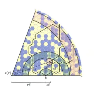
Consider the sector of angle 7r + a as a union of a sector of angle 7c with a sector of angle a. Divide the sector of angle a into [(1 - r)a-1] curvilinear quadrilaterals of radial dimension a, as shown in Figure 1-6. Let s e {1,..., [(1 - r)a-1] } and note that the event C+a(r,1) \ C,(r, 1) entails the existence of a quadrilateral of

distance sa from the inner circle of radius r such that there is a three-arm crossing of alternating colors of the half-annulus with inner radius a and outer radius sa A

(1- r - (s + 1)a).

In the case sa < (1 - r) /2, there is also a two-arm crossing from the annulus of

inner radius sa and outer radius sa

+

(1 - r) /2, then the probability that both of these events occur isO (( 2 O( a) by Proposition 1.3.5. Applying a union bound over s we obtain

P6(C a (r,1) \C2(r,1)) < ca log-1 a. (1.3.7)

Since C2(r,1) c C2+a(r,1), (1.3.7) implies

P" (C7+a(r,1)) P6(C (r,1) + ca log a-'

< c(r + alog a-).

In the case sa > (1 - r)/2, the event C2+a(r,1)

\

a log a1) in this case as well.

Ia Ia

(a) (b)

Figure 1-6: The cases (a) sa < (1 - r)/2 and (b) sa > (1 - r)/2 for the event

Cl+a(r, R)

\ Cl(r, R) in Proposition 1.3.6.

Finally, to show that 60 may be taken to be independent of r and R, we

ap-ply a multiplicative argument. Let K > 0 be large enough and 60 small enough

that P6(C,(r, R)) < (1/K)1-E for all 0 < 3 < 6o. Insert concentric arcs of radii r, rK, rK2,..., rK[1[K(R/r)J between the arcs of radii r and R, and consider the

re-gions between successive pairs of these arcs. Since a crossing from the arcs of radius r to the arc of radius R implies that each of these regions is crossed, we have

[logK(R/r)J

P(C+a(r, R)) ~ P8 (C7+a (rKkrKk+))

k=1

< c.

Remark 1.3.7. In particular, by taking r = 6, the previous results yields bounds for half-disk crossing probabilities for z E af.

Using Smirnov's theorem, we can generalize one-arm estimates to annulus sec-tors of any angle.

Proposition 1.3.8. For every e > 0,

P6(C1(r, R)) < . (1.3.8)

=_ - -, - - __ - 77 __ - ---- - - - ,

Proof. Smirnov's theorem implies that for all r and R there exists do =do (r, R, e) >

o

previ-ous proposition, we can remove the dependence on r and R with a multiplicative argument.

We can generalize the previous results for annular regions to a neighborhood of a meeting point of two analytic arcs. We let Ck "(r, R) denote the event that there exist k disjoint crossings of alternating color contained in Q and connecting the circles of radius r and R centered at z. We have the following corollary of Propositions 1.3.6 and 1.3.8.

Corollary 1.3.9. Let E > 0, let a = a (E) be an angle satisfying the conclusion in

Proposition 1.3.6. Let Q be a piecewise analytic Jordan domain in R2. Fix z E af and suppose that z is not a corner of Q. Let Ro = Ro (z, e) > 0 be sufficiently small

that BR0 (z) n f2 is contained in a sector centered at z and having angle 7r + a and

radius Ro. Then for all k e {1,2,3} and for all 0 < r < R < Ro,

P6~ ~ (p ~

k(k+1)16-Pa5(Cz(r',R)) < (1.3.9)

with implied constants depending only on E.

Proof. Since the event Co (r, R) implies a crossing of a sector of angle 7r + a with inner and outer radii of r and R,

p6 (Ck (r, R)) < p6( (rR)

and we can estimate the probability on the right by Proposition 13-6 for k 12, 31

or Proposition 1.3.8 for k = 1. E

We conclude this section by recording a generalization of the previous corollary for corners z E M . The proof of this proposition uses convergence of the

explo-ration path to SLE6. We know how to remove this dependence on SLE results only

when k = 1, where Smirnov's theorem suffices. We use (1.3.10) when k e {2, 3} only to handle the case where Q has reflex angles and to obtain the sharp exponent discussed in Remark 1.2.2.

Proposition 1.3.10. Suppose that z E Mf is a corner of Q, but otherwise the

hy-potheses and variable definitions are the same as in Corollary 1.3.9. Then the con-clusion holds, with (1.3.9) replaced by

p~l pk~zr )k(k+1)

/120-PoC~~,R)) < (1.3.10)

where 27r0 is the angle formed by aQ at z.

Proof. Define a (r, R) to be the probability of k disjoint crossings of alternating color from inner to outer radius in {z : arg z E (0,2W) and r < IzI < R}. In [75],

it is shown that

lim4a52(1, R) -Rk(k+1)/6+o(1), (3

6-+0'

using the convergence of the percolation exploration path to SLE6. By the invari-ance of the law of SLE₆ under the conformal map z - z20, we conclude that (1.3.11)

generalizes to

lim ae6(1, R) - Rk(k1)/120+o(1).

6-40 '

The following multiplicative property is also used in [75]: for all k < r < r' < r", we have

a)~j1 2 (r, r") < a 2(r, r')a? 2(r', r"). (1.3.12)

This inequality still holds with 1/2 replaced by 0. The proof in [75] for the case 6 = 1/2 relies only on these two facts and therefore generalizes to (1.3.10) for the sector domain {z : arg z E (0,2iO)}. The extension of this result to piecewise real-analytic Jordan domains with positive interior angles is obtained by following the same argument carried out in Corollary 1.3.9 for 0 = 1/2.

1.4 Proof of Main Theorem

1.4.1 Background and set-up

We begin by recalling few definitions and facts from complex analysis and differ-ential geometry. See [1], [71], and [34] for more details. If a, b E C are linearly independent over R and P is a parallelogram with vertex set {0, a, b, a + b}, then a function f : P -+ C U {oo} is said to be doubly-periodic if f(z + a) =

f(z)

f(z)

If f is continuous, then such a function may be extended by periodicity to a con-tinuous function defined on C. An elliptic function is a doubly-periodic function whose extension to C is analytic outside of a set of isolated poles. Given distinct points P1, P2 E P, there exists an elliptic function f with simple poles at pi, P2 (and no other poles) [71, Proposition 3.4]. One way to obtain such a function is to define the Weierstrass product

(jk) = Z2 aj +bk, aj bk 2(aj+bk)2 (j,k)$ (0,0) and set - a((4 - (P1 + P2)/ 2))2 Or(( -P1)o-(( - P2).

We recall the definitions of the differential forms dC = dx + i dy and d( = dx

-i dy. Note that d A d( = 2idA, where dA is the two-dimensional area measure and

A is the usual wedge product. Recall that the exterior derivative d maps k-forms to

(k + 1)-forms and satisfies

df = af d( + afd, and d(fd() = df Ad( (1.4.2) for all smooth functions

f.

Let 0 : (0, x(1), x(r), x(r 2)) -+ (T,1, r,T2) be the unique conformal map from

Q to the equilateral triangle T with vertices 1, r, and r2 which maps x(rk) to Tk for

k E {0, 1, 2}. Let S > 0 be small and define f2edge to be such that L2 \ i2edge is the set of all hexagonal faces of (12,)* completely contained in f2. Let Tedge be the image of fecige under 0.

We modify G5 to obtain a function G' for which the lattice points on the bound-ary of f2 \ f2edge are mapped to the boundary of T. Specifically, we set

Tk _{z is adjacent to} x(rk)

(Z) proj (G(z), [rk, Tk+1]) if z is not adjacent to x(rk)

G but is adjacent to [x(rk+1), X(Tk+2)]

G6 (z) otherwise,

where we are using the notation proj(z, L) for the projection of a complex number z onto the line L c C. Now linearly interpolate to extend 06 _{to a function on f2,}

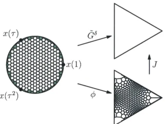
and define J : T - T by J(w) - 06(0-1(w)).

Schwarz-reflect 17 times to extend J to the parallelogram P in Figure 1-8. For example, if r is the reflection across the line through 1 and r, then for w in the triangle r(T), we define J(w) = r o J o r(w). Define an elliptic function gw via (1.4.1) with period parallelogram P and poles at p1 = wo (1 + r 2) /3 and P2 = w varying over the grey triangle K in Figure 1-8.

Figure 1-7: The function J is defined as the composition of 6_{5 with the inverse of}

the Riemann map from Q to the triangle. The region Tedge is the image under the conformal map 0 from Q to T of the region f2edge, shown in green.

. .. ...

J

X(T)

DX()

We will also need a result from the theory of Sobolev spaces. If U c R2 is a bounded domain, and 1 < p < oo, we define the Sobolev space W1'P (U) to be the set of all functions u : U -+ R such that the weak partial derivatives of u, j, and

are in LP (U); see [16] for more details. We equip W"-P(U) with the norm

IIUIIW1,P :_ II I(PU)+)- _{'lull' +} LP(11) _+~

Denote by id the identity function from P to P, and define C' (P) to be the set of smooth, real-valued functions from P. Since

J

takes vertices to vertices and boundary segments to boundary segments, J - id is continuous and doubly-periodic. Since smooth functions are dense in W1 1 (P) and L* (P) [16], for each e > 0 we obtain a pair of smooth functions Q1, Q2 E C' (P) such that

IQ(w) - (1(w) - w)I < e for all w E P,

I|Q1

11 Q2 - Im(J - id) Ilwi < E,

where Q = Q1 + iQ2 (for see [16] 5.3.3 and C.5, for example). Defining Q, and Q2

to be bump function convolutions, we arrange for Q, and Q2 to inherit periodicity from

J

aQ - a(J -- id)IIgwI dA <C', (1.4.4)

where dA refers to two-dimensional Lebesgue measure. One way to see this is to define f(z) = aQ(z) - a (J(z) - z) and note that for R > 0, we have

Hf9HLi

By the dominated convergence theorem, we may choose R sufficiently large that

the second term on the right-hand side is less than e'/2. Once R is chosen, we may choose Q so that IIfIILi <; E'/(2R), by (1.4.3). Then (1.4.4) follows from (1.4.5).

1.4.2 Proof of main theorems

Proof of Theorem 1.2.1. The following calculation is similar to the proof of the Cauchy

integral formula, but with two key changes: we keep track of the 3 term, and we use the elliptic function gw in place of the usual kernel '-4 1

/(.

and apply Stokes' theorem to the region P \ (B1U B2) to obtain that for smooth,

P

T2

Figure 1-8: We extend J(w) to a function on the parallelogram P, which is a union of 18 small triangles. The elliptic function gw : P - C has poles at wo fixed and w

varying in the gray region.

complex-valued, periodic functions Q on P, we have

_,_.Q(()gw(( ) d(- Q(C )gw(C ) dC \(1B

Note that the integral around af2 vanishes by periodicity. Applying (1.4.2) and the product rule, we obtain

P\(IUB) P(BB2)[(a Qd( + aQdk)gw + (agwd( +

agd)]A

JP\( B1 UB 2 ) ~P\ (B1u B2)gdD]

Jp\ fBu₂ aQ(() gw(() d A d(,.

=P\VB1UB2)

Let

Q

theorem. We obtain

27riQ(w) Res(gw,w) + 2iriQ(wo) Res(gw,wo) = 2i jaQ()gw(() dA((), (1.4.6) where dA (4) = dx dy is notation for the area differential. The key step of the proof is to bound the right-hand side of (1.4.6) by O(6c). To do this, we first consider

j in place of Q, and we estimate the integral over the regions T \ Tedge and Tedge

separately. We postpone the details of these calculations to the following section, along with stronger lemma statements (Lemmas 1.5.2 and 1.5.4).

Lemma 1.4.1. There exists c > 0 so that

'Tedge aj(4)gw(()dA(() = 0(6'), (1.4.7)

where the implied constants depend only on the three-pointed domain. Lemma 1.4.2. There exists c > 0 so that

fTe(()gw(()dA(()

JT\Tedge

where the implied constants depend only on the three-pointed domain.

Since Res(gw, w) is a continuous function of w with no zeros in K, there exists C > 0 such that

0 < C-1 < Res(gww) < C < oo, Vw E K,

and similarly for the residue at wo. Therefore, (1.4.8) implies that Q(w) is within 0(6c) of a constant function, as w ranges over the gray triangle shown in Figure

1-8. By considering w to be one of the vertices of the gray triangle (so that

J(w)

-w = 0), we see that this constant function is 0(6c). We conclude that Q(w) =

0(6c). By (1.4.3), this implies J(w) - w = O(SC). By definition, this is equivalent

to 05(z) - O(z) = 0(Sc). The theorem follows, since 0 agrees with G1 except on

the outermost layer of lattice points. [

We combine the rate of convergence for H1 + THT + r2HT2 with the rate of

con-vergence for H1 + HT + HT2 near iM to prove the rate of convergence of the crossing

probabilities.

Proof of Theorem 1.1.1. Let z E [x(1), x(r)]. First we note that H 2(z) = O(C) by

Proposition 1.3.4. Hence, by Theorem 1.2.1,

Hi(z) + rHT(z) = O(z) + O(SC) .

We also have that

Hl(z) + HT (z) = 1 + (O(5c),

since S6(z) = 1 + 0(6C) by Proposition 1.3.4 (ii). Since the vectors (1,1), (1, r) E C2

are linearly independent, this concludes the proof. E

1.5 Bounding the error integral

1.5.1 Piecewise analytic Jordan domains

In this section, we prove the two lemmas used in the proof of the main theorem. We often treat the conformal map O(z) like a power of z when z is near a corner

of the domain Q. To make this precise, we use the following theorem from the conformal map literature [35].

Theorem 1.5.1. If Q is a Jordan domain part of whose boundary consists of two analytic arcs meeting at a positive angle 27ra at the origin, and if 0 : Q -+ H is a

Riemann map sending 0 to 0, then there exists a neighborhood B of the origin and continuous functions Pi, P2 B n Ti -+ C and p3, p4 :(B n 11) - C for which

(Z) = z1/(2a)p1(z), 0'(z) = z1/(2a)- 1p2(z),

0--1(z) = z2a p3(z), and ($-1)'(z) = z2"1p 4(z)

and p;(0) 7 0 for i c {1, 2,3,4}.

We choose a collection B of disks covering the boundary of Q as follows (see Figure 1-9). For each z e DO, choose a disk B(z) centered at z and small enough that the boundary arc (or arcs) containing z admits a Taylor expansion in B (z). If

necessary, shrink B(z) so that U2 is well-approximated by its tangent (or tangents, if z is a corner point) in B(z), in the sense of Propositions 1.3.6 and 1.3.10. If nec-essary, shrink B (z) once more to ensure that 12 n B (z) has one component. From this collection of open disks, extract a finite subcover B = (Bj){ 1 of aQ containing

Bcorners = {B(z) : z is a corner point}. Then 13 is an annular region whose interior

has positive distance from aQ. Thus, for all sufficiently small 6, B covers fedge.

Note that this cover has been chosen in a manner which depends only on Q and c, and in particular is independent of S.

Throughout our discussion, we permit the constants in statements involving asymptotic notation to depend only on the three-pointed domain. We also use C to represent an arbitrary constant which depends only on the three-pointed do-main. When working with the variable E, we will frequently relabel small constant multiples of E as E from one line to the next.

Lemma 1.5.2. Let J, gm, be as in Section 1.4, and suppose that the angle measures

at marked points are 2irai for i = 1,2,3, and remaining angles are 2np31 for j =

1,2,..., n. For every E > 0,

aj(()gw( )dA(() < 5mn'j('-61 E, 1..

fedge

.

where the implied constants depend only on E and the three-pointed domain. Proof of Lemma. Let 1 be as described above. Since the number of disks in B is bounded independently of 6, it suffices to demonstrate that (1.5.1) holds for each one. Let B E 13, and let 7r1 be the angle formed by aQ center of B.

To bound fTedgeno(nnB) aj(()gw(C)dA(() . we index all the faces {Fk} intersect-ing ai in such a way that the distance from Fk to the center of B is :: k6 for all k; this is possible since ad is piecewise smooth. We will bound the integral over each

X(1)

Figure 1-9: We cover the boundary with finitely many small disks, so that the boundary is approximately straight in each disk. Moreover, we ensure that every corner and every marked point is centered at one of these disks. More disks are required in regions of high curvature, as illustrated here for a domain bounded by a limaeon.

k+1

Figure 1-10: If z is adjacent to the side [x(rk+l) x(.rk+2)], then the distance from

G6(z) to a T is equal to the probability H~k(z). This probability is bounded by that of a two-arm half-plane event with radius k6 and the two-arm P-annulus event with inner radius 2k& and constant-order outer radius.

Fk and then sum over k (see Figure 1-10). Let ( e Tedge n ((Fk) and suppose that [r, T2] is the closest boundary arc. We rewrite

J(O) = 61(1((O))( A-1)(, (1.5.2)

and we define z =- 1((). First we bound 0'5(z). In modifying G,5(z) to obtain

0,"(z), the image of z has to be moved no farther than H,1(z) = P(E₁(z)), by the definition of G'(z). The event E₁(z) entails a two-arm half-disk crossing and a two-arm fp-annulus crossing (see Figure 1-10). Since these events occur in disjoint regions, they are independent and we can bound P(E1(z)) by the product of their

probabilities. By Corollary 1.3.9, the two-arm half-plane exponent in Q, is 1 and by Proposition 1.3.10 the two-arm P-annulus exponent is 1/2P. Thus the probability of E1(z) is at most (k6)1/ 2P-E (1/k)1 . Hence for z + 17 in the outermost layer and

z a neighbor of z + q, we have (d'(z + 7j) - 66 (z)) 1

(C

In the last step we use a shifted domain trick (see the proof of the second in-equality in Proposition 1.3.3 and Figure 1-5) and apply the trivial inin-equality P(A

\

-W z), we get 61d5 (z) 6-1 (k)1/2_P-E

(1/k)1-E.

We assume that the location z of the pole is in the face nearest to the center of

B (since that is the worst case) and also that the image of the center of B is not a

vertex of the equilateral triangle T. We obtain

'Tedgeos(OnB j) J(()gw (()dA(4) (1.5.4)

C1/6

< 1 sup Ia05(z)(0-1)'(O(z))gw(q-1 (z)) area(0(Fk))

k=1 ZEFk

by replacing the integrand with its supremum on each Fk and summing over k.

estimate the factors involving (. We bound the right-hand side of (1.5.4) by S(c(r)'('P(z)) gw area(P(Fk)) C/6-__________ A_____ < -1 (ko) 1/2p-E (1/k)1- (51-1/2 2M -1 /2P 52 ( 2/2 -2 k=1 C/6 61-E y () 1 /2P-24) (k=1 6 1' if 2P< 1 61/2p-Eci P>1

We have evaluated the sum by noting that the factor in parentheses is a convergent Riemann sum when the exponent is at least -1. When the exponent is less than

-1, the summation over k gives a constant factor, leaving the contributions of the

powers of S.

If the center of By is a marked point, the proof is essentially the same and the net

effect is to replace 1/2P with 1/6a throughout the calculation. These replacements are justified either by fewer percolation arms (when the exponent appears in an arm event estimate), or by the angle of 7r/3 at the vertices of the triangle T (when the exponent appears because of the conformal map r).

Remark 1.5.3. We can remove the dependence on SLE by using Smirnov's theorem to estimate one-arm

p-annulus

6mini ,1 (1.

,)

Lemma 1.5.4. Let J,gm, {ai}, {pj} be as in the statement of Lemma 1.5.2. Let C3 =

2/3 be the 3-arm whole-plane exponent. Then

<Mii(C3, E

T\Tedge aJ(()gw(()dA(() ,< 6

' 'R' ,(1.5.5)

where the implied constants depend only on e and the three-pointed domain.

Proof of Lemma. We will use Proposition 1.3.3 to bound aG. Let B be as above and

note that dist(aO, Q \ U B) > 0 by the discussion preceding Lemma 1.5.2.

We first handle Q

\

occurs, say E1,,arm(z). Let b be the point nearest x(r2) where a blue arm touches down in the shifted domain, and let s be the number of lattice units along the boundary from b to x(r2). When z t U 3 (see Figure 1-11), z is well away from the

boundary thus we note that such a five arm event entails the existence of:

1. a 3-arm whole-plane event in alternating colors at z, in a ball of radius 0(1),

2. a 3-arm half-annulus event of alternating colors originating at b, in a semi-circle of radius s&/2, and

X(1)

Figure 1-11: To bound the probability of the five-arm difference event described in Proposition 1.3.3, we consider three regions which contain two-arm or three-arm crossing events (these regions are shown in green and red, respectively).

3. a 2-arm half-annulus event in an annulus of inner radius s6/2 and outer

ra-dius 0(1).

Since the derivative of the conformal map is bounded above and below for z away from the boundary, we can ignore the contribution of '(-1(z)) in (1.5.2) and calculate

3-arm whole-plane 3-arm half-plane 2-arm half-ann. C/6 J J(z) I,< 45-1 (15C3-E) X (1/S)2 X (S6) s=1 <6 C3-E. Hence we have <p aB3J(()gw(( )d A (( )

<

To bound the integral of the union of the balls in B, we handle each B E 8 separately. We first consider a ball centered at a marked corner, say x(r). Once again, for each z and each percolation configuration, we define b E a)f to be the point nearest x(r2) at which a blue arm from z touches down in the shifted domain. This time we let s be the graph distance from b to the boundary point zfoot nearest to z (see Figure 1-14) and index the faces Fn,k in such a way that if z E Fn,k,

Ix(r)

Ia

I

C

Figure 1-12: We sum over the possible locations for b, considering the cases b E A,

b E B, b

E

arc [x(T), x(r2)] than to the boundary arc [x(1), x(r)].

Suppose that the corner at B is one of the three marked points and has inte-rior angle air. We bound I a by summing over all possible locations for b. We consider four cases:

" Case A: b is closest to the corner at x(r) (Figure 1-13(a)),

" Case B: b is within k/2 units of zfoot (Figure 1-13(b)),

" Case C: b is more than k/2 units to the right of zfoot but closer to zfoot than to x(r2) (Figure 1-13(c)), and

" Case D: b is closest to x(r2) (Figure 1-13(d)).

For simplicity, we assume that [x (r), x (r2)] is a real analytic arc (that is, that there are no corners between x(r) and x(T2_{)). It will be apparent that similar estimates}

hold when additional corners are accounted for.

Denote by P(z, b) the contribution to aG of the five-arm event with missed connection at b (see Figure 1-5). As in (1.5.4), we bound the sum for Case A by a constant times

P(z,b)

C/5 Ck k/22 r )/2a-e

N-11-' k .N

k=1 n=1 r=1 ; 3-arm disk. 3-arm half-disk- 1-arm a-ann.

2-arm a-ann.

(0-1)'(o(Fn,k)) area(O(Fn,k))) gw x (k)1-1/6a 42(k)1/3a-2 (k)-1/6a

We upper bound the contribution of Case B by a constant times

P(z,b)

C/S Ck k/2 _{1 /S2 i12}

-=1

n-c3- (kk1/

2-k= n1 =133-arm disk _{V 1-arm a-ann.} 3-arm half disk 2-arm half-ann.

($-1)'(*Fn,k)) area(O(Fn,k)) gw

x (ki5)1-1/6a 62(k,6)1/3a--2 (kM)-1/6a

< min(C3,1/6a)-E.

For Case C, we get

P(z,b) C/S Ck C/S

4

-k=1 n=1 r=k/2 3 _{3-arm disk. 3-arm half-disk} < 1/6a--.

(k45)1-1/6a52(kS5)1/ 3a-2

(k45)

For Case D, we denote by 27ry the angle at x(r2) and by t the number of lattice units from x(T2 ) to b. We obtain P(z,b) C/S Ck C/S.

S1

-k=1 n=1 t=1 _{3-arm disk. 3-arm half-disk- 2-army ann}

The proofs for the bounds in a disk whose center is not marked are essentially the same as these. As in the proof of Lemma 1.5.2, the net effect is to replace 1/6a

with 1/2p. El

Remark 1.5.5. As in Remark 1.5.3, we can remove the dependence on SLE by using Smirnov's theorem instead of Proposition 1.3.10, under the additional assumption that ai has no reflex angles (that is, maxij(ai, i) < 1/2). By using the weaker

one-arm fi-annulus bound in place of the two-one-arm and three-one-arm bounds, we obtain

(1.5.5) with the right-hand side replaced by

mini, C3, 1

Without the help of SLE, our techniques break down in the presence of reflex an-gles.

(1)4 V,

0*

Figure 1-13: Assuming that z is near a marked corner, we have four cases to con-sider: (a) b is close to x(r), (b) b is close to z, (c) b is between z and x(r2) but far

from both, and (d) b is close to x (r2). For a closer view of the corner with additional labels, see Figure 1-14.