Deformation capacity of reinforced concrete columns

Publisher’s version / Version de l'éditeur:

ACI Structural Journal, 106, 2, pp. 187-195, 2009-03-01

READ THESE TERMS AND CONDITIONS CAREFULLY BEFORE USING THIS WEBSITE.

https://nrc-publications.canada.ca/eng/copyright

Vous avez des questions? Nous pouvons vous aider. Pour communiquer directement avec un auteur, consultez la

première page de la revue dans laquelle son article a été publié afin de trouver ses coordonnées. Si vous n’arrivez pas à les repérer, communiquez avec nous à PublicationsArchive-ArchivesPublications@nrc-cnrc.gc.ca.

Questions? Contact the NRC Publications Archive team at

PublicationsArchive-ArchivesPublications@nrc-cnrc.gc.ca. If you wish to email the authors directly, please see the first page of the publication for their contact information.

NRC Publications Archive

Archives des publications du CNRC

This publication could be one of several versions: author’s original, accepted manuscript or the publisher’s version. / La version de cette publication peut être l’une des suivantes : la version prépublication de l’auteur, la version acceptée du manuscrit ou la version de l’éditeur.

Access and use of this website and the material on it are subject to the Terms and Conditions set forth at

Deformation capacity of reinforced concrete columns

Mostafaei, H.; Vecchio, F. J.; Kabeyasawa, T.

https://publications-cnrc.canada.ca/fra/droits

L’accès à ce site Web et l’utilisation de son contenu sont assujettis aux conditions présentées dans le site LISEZ CES CONDITIONS ATTENTIVEMENT AVANT D’UTILISER CE SITE WEB.

NRC Publications Record / Notice d'Archives des publications de CNRC:

https://nrc-publications.canada.ca/eng/view/object/?id=91b23fcf-1f66-4d9f-91fd-7a5887de54bf https://publications-cnrc.canada.ca/fra/voir/objet/?id=91b23fcf-1f66-4d9f-91fd-7a5887de54bf

http://irc.nrc-cnrc.gc.ca

De for m at ion c a pa c it y of re inforc e d c onc re t e c olum ns

N R C C - 5 1 2 1 9

M o s t a f a e i , H . ; V e c c h i o , F . J . ; K a b e y a s a w a , T .

M a r c h 2 0 0 9

A version of this document is published in / Une version de ce document se trouve dans: ACI Structural Journal, 106, (2), pp. 187-195

The material in this document is covered by the provisions of the Copyright Act, by Canadian laws, policies, regulations and international agreements. Such provisions serve to identify the information source and, in specific instances, to prohibit reproduction of materials without written permission. For more information visit http://laws.justice.gc.ca/en/showtdm/cs/C-42

Les renseignements dans ce document sont protégés par la Loi sur le droit d'auteur, par les lois, les politiques et les règlements du Canada et des accords internationaux. Ces dispositions permettent d'identifier la source de l'information et, dans certains cas, d'interdire la copie de documents sans permission écrite. Pour obtenir de plus amples renseignements : http://lois.justice.gc.ca/fr/showtdm/cs/C-42

DEFORMATION CAPACITY OF REINFORCED CONCRETE

COLUMNS

Hossein Mostafaei1 , Frank J. Vecchio2 and Toshimi Kabeyasawa3

1. Postdoctoral Fellow, Dept. of Civil Engineering, Univ. of Toronto, ON, Canada, M5S 1A4 2. Professor, Dept. of Civil Engineering, Univ. of Toronto, ON, Canada, M5S 1A4, 3. Earthquake Research Institute, the University of Tokyo, Tokyo, 113-0032, Japan

Biography: Hossein Mostafaei is a Postdoctoral Fellow at the Department of Civil

Engineering, University of Toronto. He obtained his Ph.D. in Structural/Earthquake Engineering from the University of Tokyo on March 2006. His research interests include displacement-based methodology, analytical and numerical modeling of reinforced concrete elements, seismic performance assessment and rehabilitation of reinforced concrete structures.

Frank J. Vecchio, FACI, is a professor at the Department of Civil Engineering, University of Toronto. He is a member of Joint ACI-ASCE Committees 441, Reinforced Concrete Columns, and 447, Finite Element Analysis of Reinforced Concrete Structures. His research interests include: nonlinear analysis and design of reinforced concrete structures; constitutive modeling; and assessment, repair, and rehabilitation of structures.

Toshimi Kabeyasawa is a professor at Earthquake Research Institute, The University of Tokyo. He is an active member of various committees in Japan Concrete Institute, Architectural Institute of Japan, and Japan Building Disaster Prevention Association. His research interests include reinforced concrete structures, seismic performance evaluation, retrofit of existing structures, and structural dynamics.

ABSTRACT

An effective approach is presented for estimation of the ultimate deformation and load capacity of reinforced concrete columns based on principles of axial-shear-flexure interaction. Conventional section analysis techniques are employed for modeling the flexure mechanism, and the simplified Modified Compression Field Theory is implemented for modeling the shear behavior of elements. Average centroidal strains and average concrete compression strains derived from the flexural model are implemented in the shear model, and used to calculate shear deformation and concrete strength degradation. This approximate procedure can be easily implemented in a hand-calculation method in a few steps. The approach is employed for estimation of the ultimate deformation of shear- and flexure-dominated reinforced concrete columns previously tested. The analytical results are compared with the experimental data and consistent strong agreement is achieved.

Keywords: column, ductility, ultimate deformation, axial-shear-flexure interaction, displacement-based evaluation, axial deformation, ultimate strength

INTRODUCTION

Although the behavior of reinforced concrete columns and beams has been studied for more than 100 years, the problem of estimating ultimate deformation at ultimate strength, or the lateral deformation at shear failure, remains unsolved. Experimental studies by various authors1,2 revealed that reinforced concrete columns subjected to axial load and lateral load with similar ultimate strength may fail in significantly different ultimate deformations. Although it is agreed that increasing the ratio of the transverse reinforcement will enhance the ductility of a column, determining the ultimate deformation at which the element fails in shear is still a major challenge for engineers. Based on newly introduced performance-based

design philosophies for response estimation of structures, one of the main performance properties in the design process is the ductility and deformability of the structure. The more ductility the structure possesses, the better the performance and the more economical the design. Therefore, it is essential to have and apply a suitable analytical tool to accurately estimate the ultimate deformation or ductility of reinforced concrete column elements.

Recently, an attempt was made to include the effects of shear deformations in sectional analyses through the Axial-Shear-Flexure Interaction (ASFI) method3,4. The ASFI method was developed to improve not only the response simulation of reinforced concrete elements with dominant shear behavior, but also to improve the flexural response calculation capabilities of the fiber model approach. This was done by satisfying compatibility and equilibrium conditions for both the flexure and shear mechanisms employed in the ASFI method. In the approach, the flexure mechanism was modeled by applying traditional section analysis techniques, and shear behavior was modeled based on the Modified Compression Field Theory (MCFT)5. The approach was implemented and verified for a number of reinforced concrete columns tested with different axial loads, transverse reinforcement ratios, longitudinal reinforcement ratios, and scales ranging from one-third to full-scale specimens. However, the application of the MCFT, as a shear model within the ASFI method, requires relatively intensive computation; a calculation process involving inversion of a 3×3 matrix, and an iteration process, converging five different variables, which might not be suited to engineers in practice. In addition, the results of analyses by the ASFI approach suggested further studies on the onset of shear failure or ultimate deformation of reinforced concrete columns.

Considering the fact that columns with either dominant flexure or shear response fail finally in shear, the main objective of this study is to provide a simple analytical model, applicable for design in practice, for determining the critical conditions that result in the shear failure of

reinforced concrete columns and the corresponding ultimate strength and deformation capacity. In the new analytical process, tension-shear failure across cracks, loss of concrete compression strength, and compression-shear failure are the main failure mechanisms considered at the ultimate state for both shear-and flexure dominant members. In addition, crushing of cover concrete, bond failure, buckling of compression bars, and rupture of reinforcement are other potential failure conditions and must be checked at the ultimate state.

RESEARCH SIGNIFICANCE

Accurate estimation of the ultimate deformation and ductility of reinforced concrete elements has long been a significant challenge and aim of researchers. A new approach is developed to estimate both the ultimate deformation and load capacity of reinforced concrete columns and beams. The proposed method can be used as an effective analytical tool for the purpose of displacement- and performance-based design.

ASFI METHOD AND UNIAXIAL SHEAR-FLEXURE MODEL

The Axial-Shear-Flexure Interaction (ASFI) Method is composed of two models: a flexure model based on traditional uniaxial section analysis principles, and a shear model based on a biaxial shear element approach. The total lateral drift of a column between two sections, γ, is the sum of shear strain, γs, and the flexural drift ratio, γf, between the two sections.

Furthermore, the total axial strain of the column between the two sections, εx, is the sum of

axial strains due to axial, εxa, shear, εxs, and flexural, εxf, (Fig.1) mechanisms.

f s γ γ γ = + (1) xf xs xa x ε ε ε ε = + + (2) The centroidal axial strain, εxc, is derived from a section analysis or axial-flexure model, and

is defined as the sum of the strains due to axial and flexural mechanisms, εxc = εxaf + εxf. On

the other hand, from the shear model for axial-shear elements, the sum of the axial strains due to axial and shear mechanisms is determined, εs= εxas+ εxs. As a result, to obtain εx in Eq. (2),

εxf must be extracted from εxc and added to εs, considering εxa = εxaf = εxas.

Equilibrium of the shear and axial stresses from the axial-flexure model, τf and σxf, and from

the axial-shear model, τs and σxs, respectively, must be satisfied simultaneously through the

analysis. That is,

o xs

xf σ σ

σ = = (3)

τ_f =τ_s =τ (4) where: σxf = axial stress in the axial-flexure mechanism, σxs = axial stress in the axial-shear

mechanism, σo = applied axial stress, τf = shear stress in the axial-flexure mechanism, τs =

shear stress in the axial-shear mechanism, and τ = applied shear stress. Stresses in axes perpendicular to the axial axis of the column, the clamping stresses σy and σz, are ignored due

to equilibrium between confinement pressure and hoops stresses. 0

= = _z

y σ

σ (5) Fig. 2 illustrates the two models for axial-shear and axial-flexure, and their interactions, by means of springs in series. Fig. 3 illustrates the ASFI method, for a reinforced concrete column with two end sections, including the equilibrium and compatibility conditions. The total axial deformations considered in the ASFI method are axial strains developed by axial, shear and flexural actions, and by pull-out mechanism.

In a uniaxial shear-flexural model, applied in this study, compatibility is also satisfied for average concrete compression strains. Consider a reinforced concrete column of moderate height, fixed against rotation and translation at the bottom and free at the top, subjected to in-plane lateral load and axial load as shown in Fig. 4. Given its pattern along the column (see Fig. 4-a), the concrete principal compression strain for an element between two sections,ε2,

may be determined based on average values of the concrete uniaxial compression strains corresponding to the resultant forces of the concrete stress blocks.

) ( 5 . 0 1 2 2 2 = ε i +ε i+ ε (6) This is the main hypothesis of the new method proposed here; this assumption simplifies the shear model significantly from a biaxial to a uniaxial mechanism. For the column in Fig. 4, the compression strain obtained from the above equation is set equal to the average principal compression strain of the element between the two sections of i and i+1.

MODIFIED COMPRESSION FIELD THEORY

The shear mechanism in the ASFI method, as well as in this analytical process, is modeled according to the Modified Compression Field Theory (MCFT)5. It is a suitable displacement-based evaluation approach for predicting the load-deformation response of reinforced concrete membrane elements subjected to shear and normal stresses. The MCFT is essentially a smeared rotating crack model. It includes compression softening effects, tension stiffening effects, and consideration of local conditions at cracks. The MCFT is based on orientations of the principal average strains in an element leading to the calculation of principal average stresses in concrete through concrete constitutive relationships. Transforming the average concrete principal stresses to the global coordinate axes and adding to the average stresses in the reinforcement gives the total average stresses in the element. There are two checks in the calculation process relating to the crack zones. The first is to ensure that tension in the concrete can be transferred across the crack. The second is to ensure that the shear stress on the surface of the crack dose not exceed the maximum shear resistance provided by aggregate interlock. A reinforced concrete element within the context of the MCFT can be illustrated by the free body diagram of the membrane element depicted in Fig. 5.

DERIVATION OF THE ANALYTICAL MODEL

Considering the free body diagram of the membrane element in Fig. 6, equilibrium conditions in the MCFT require that:

sx sx cx x f ρ f σ = + (7) sy sy cy y f ρ f σ = + (8) where, for beams and columns σ_x is the total normal stress in the x-direction (i.e., the

applied axial stress), σ_y is the total normal or clamping stress in the y-direction, taken to be zero, and are stresses in concrete in the x (axial) and y (transverse) directions,

respectively,

cx

f f_cy

sx

ρ and ρ_sy are the reinforcement ratios in the x (axial) and y (transverse) direction, respectively, and and are the stresses in the main bars (axial direction) and in the transverse reinforcement (y direction), respectively.

sx

f f_sy

A Mohr’s circle for concrete stress yields the following equilibrium relationships:

c s c cx f f = ₁−τ cotθ (9) c s c cy f f = ₁−τ tanθ (10) ) tan / 1 (tan 1 2 c s c c c f f = −τ θ + θ (11) where is the concrete principal tensile stress, is the concrete principal compressive stress, 1 c f s 2 c f

τ is the concrete shear stress, and θ_c is the crack angle.

On the other hand, the compatibility equation based on the Mohr’s circle for strain requires that: 2 2 2 tan ε ε ε ε θ − − = y x c (12) y x ε ε ε ε₁+ ₂ = + (13) where ε_x is the axial strain, ε_y is the strain in the transverse reinforcement, ε₁ is the

concrete principal tensile strain and ε₂ is the concrete principal compression strain.

With εx obtained from section analysis, combining Eqs. (9), (10), (12) and (13) yields two

useful equations for estimation of ε_y and ε₁.

yy y

y b c b ε ε

ε = 2 + − <

(14) where εyy is the yield strain, and

s sy c cx c x s sy c E f f f 2)( c E f b ρ ε ε ε ε ρ 1 2 1 1 2 ) ( , 2 2 + − − = − =

where, Es is modulus of elasticity of transverse reinforcement. When strain in the transverse

reinforcement is greater than the yield strainε_yy, Eq. (15) can be applied:

yy y x syy sy c cx c x f f f f _{ε ε ε} ρ ε + )( 1 2 ε ε = − − + ≥ ) ( ) ( ₁ 1 (15)

where is yield stress of transverse reinforcement, is determined based on Eqs. (7). At the ultimate states, Eq. (15) is usually the governing equation. Given

syy

f f_cx

β as the concrete compression softening factor, an average initial value of f_c1 = 440. f_t′ can be considered for Eqs. (14) and (15), by assuming a tension stiffening model and an average tensile strain ε1

which can be derived from Eq. (16) based on an upper bound of β ≤1 and lower bound of 2 . 0 ≥ β . 0 . 1 34 . 0 8 . 0 1 1 ≤ ′ − (16) = β c ε ε

where, εc′ is concrete peak strain. The MCFT limits the shear stress transferred by aggregate

interlock across a crack surface, τi, to the value given by Walraven’s equation:

16 24 31 . 0 18 . 0 + + ′ ≤ i g c a w f τ (MPa, mm) (17) 8

with w=s_θε₁, and y c x c s s s_{θ θ θ} cos sin 1 +

= , where and are the average crack spacings in

the x- and y-directions, respectively and ag is the maximum aggregate size. x

s s_y

Equilibrium in the y-direction, at the crack, requires that:

f_sycr =(σ_y +τ_stanθ_c−τ_itanθ_c)/ρ_sy (18) where f_sycr is the transverse reinforcement stress at the crack, and σ_y is the clamping stress which is equal to zero. Hence for f_sycr = f_syy Eq. (18) yields:

τ_max ≤τ_i+ f_syyρ_sycotθ_c (19)

FLEXURE MECHANISM

The traditional section analysis method is a handy and convenient approach for the evaluation of the flexural performance of a reinforced concrete column or beam. Since the analysis is implemented assuming a uniaxial stress field, material modeling and analytical computation are simple and a solution can be achieved with adequate convergence in a few steps. Fig. 7 shows a flexural section for a column. The force-strain relationship for a section, under uniaxial bending, can be derived from axial load equilibrium as following:

P x A E A E_{i i i i i} o

∑

∑

c s s s s i iA A E AE abE E = + ′ ′+

∑

∑

= anda=β₁c, and where β1 is the rectangular stress block

coefficient which is equal to 0.85 for f ′ <28 MPa; _c β1 is reduced continuously by 0.05 for

each 7 MPa above 28MPa. The main assumption of plane sections yields the following relationships: c d d c c h c s s o c − = ′ − ′ − = − = − − = ε ε ε β ε φ 5 . 0 ) 5 . 0 1 ( ₁ (22)

Solving Eq. (20) for ε_o and β₁ =0.85 gives:

c c s s s s c c s s s s o a bE E dA E A d abE E A E A h hP ε ε ε 1.7391 ] 5 . 0 [ 2 ] [ 7391 . 1 2 + + + ′ ′ ′ + + ′ ′ − = (23)

By determining , , and , the bending moment within the section is obtained by applying moment equilibrium for the section.

s f ′ f_s f_c c s s s sf d d A f a h baf A d d M =0.5( ′− ) ′ ′+0.5( − ′) +0.5( − ) (24) If M is the end-moment of a column, as in Fig. 3, then flexural shear stress, τ_f , is determined based on Eq. (25).

in f f L bd M = τ (25) where d ≤d_f ≤h is assumed based on the failure mode described later.

PROCEDURES FOR ESTIMATION OF ULTIMATE DEFORMATION

The main failure mechanism for both shear- and flexure-dominated beams and columns is shear failure. Fig. 8 shows specimen No.12 and No.15, from Table 1, with shear and flexure responses, respectively; however both failed in shear at the ultimate deformation. Bond failure, buckling of compression bars, rupture of the tensile bars, and crushing of cover concrete are other failure criteria for reinforced concrete columns and beams. The analytical procedure presented here is based on assuming shear failure as the main failure mechanism, and checking for the other failure criteria.

Three shear failure conditions are defined based on the MCFT as: shear failure at a crack (Failure Mode 1); failure due to loss of compression strength (Failure Mode 2); and shear-compression failure (Failure Mode 3). Shear failure at a crack, which is typically the governing case for columns with low transverse reinforcement ratios, is determined using Eq. (19) and Eq. (25). Shear failure occurs when:

_{i syy sy c} in f f f L bd M _{τ ρ θ} τ = ≥ + cot (26) where, . Columns under high shear force, such as short columns, if not failing via Mode 1, will lose compression strength, f2, due to shear deformation and fail before the peak,

d df =

c

ε

ε₂ ≤ ′. This failure condition, Mode 2, is defined by Eqs. (11) and (25) when:

) tan / 1 (tan ) ( 1 2 c c c c in f f f f L bd M θ θ τ + − ≥ = (27) where for short columns with span-to-depth ratios less than 1.0 and for columns with span-to-depth ratio more than 1.5; for ratios between 1.0 and 1.5, is determined by interpolation.

h

d_f = d_f =d

f d

Columns and beams with a ductile flexure performance, when having sufficient transverse reinforcement and relatively low shear stress, will fail in shear whenε₂ =ε_c′ via Mode 3.

in f f L bd M = τ (28) where, ε₂ =ε_c′ 15

and . Finally for flexure beams and columns with very low shear stress, especially under heavy cyclic loadings, the compression softening factor may be limited to

h d_f =

. 0 ≥

β . In other words, if β reduces to 0.15 then that will signal the ultimate state. None of the columns in Table 1 reached this limit within the range ε2 ≤εc′, hence further study is

required in regards to this condition.

Based on the shear failure criteria described above, an analytical procedure can be constructed for the estimation of the ultimate deformation of a reinforced concrete column with a flexure section at the section with maximum moment, such as the column shown in Fig.3. In step-by-step fashion, the procedure is as follows:

1. Assume an initial value for concrete compression strain of the flexure section, ε_c ; for example, εc =εc′.

2. Employ Eqs. (21), (22), and (23) to determine the centroidal strain of the section, εo,

through one or two iterations. Assume an initial value for ε_o; for example ε_o =0.001.

3. Determine the axial strain at the inflection point with zero moment, ε_xa , using basic sectional analysis principles.

4. Compute the average concrete principal compression strain ε₂ and axial strainε_x for the shear model. 2 2 xa c ε ε ε = + (29) 2 xa o x ε ε ε = + (30) 5. Using Eqs. (13), (14) and (15) determine ε₁ and ε_y. Since the problem is being solved for conditions at the ultimate state, usually the transverse reinforcement has yielded and only Eq. (15) need be applied.

6. Employ Eq. (12) to obtaintanθ_c .

7. Using Eqs. (26) (27), and (28), check for shear failure. If no failure has occurred, then increase ε_c and repeat the above steps. If, for example, Eq. (26) shows shear failure at crack, then ε_c must be reduced until all three equations provide greater or equal values.

8. Check for crushing of the cover concrete. This is not a failure model but the axial load

capacity will decline; strain hardening sometimes will help mitigate the decline. Check for buckling of the compression bars, bond failure, rupture of tensile bars, and compression softening factorβ ≥0.15.

9. Determine the ultimate deformation using Eq. (1) where, = =

∫

Lin in in f x dx L L ₀ 1 _φ δ γ , and c x s _θ ε ε γ tan ) ( 2 − ₂ =

10. Finally, the ultimate lateral load capacity is obtained by

bh

V_u =τ_f (31) If the column or beam has sufficient transverse reinforcement then the initial value for ε_c can be selected as ε_c = 2ε_c′ −ε_xa, which is the limit for Failure Mode 3. Then check for other failure modes. If this is the dominant failure mode, then determine the ultimate drift.

Confinement effects can be taken into account for both shear and flexure models based on equations provided by Park, Priestley and Gill2. Note that both the confinement factor and the compression softening factor,β, are applied in the constitutive law of compression concrete of the shear model. However, for the flexure model, only the confinement factor is considered and employed in the concrete stress-strain relationship.

NUMERICAL EXAMPLES

The analytical procedure is employed for Specimen No.12, described in Table 1, with a shear-dominant response. Units are in mm, kN, and MPa. For the secondary units, use 1 in = 25.4 mm, 1 ksi = 6.89 MPa, and 1 kip = 4.45 kN.

1. As an initial value assumeε_c =−0.002.

2. To satisfy Eq. (23), an iteration procedure can be applied with few steps. First considerε_o =0.002 anda=0.85c; hence:

) 353 . 1 353 . 2 ( _{c o} c h a ε ε ε − = or a 81mm ) 002 . 0 ( 353 . 1 ) 002 . 0 ( 353 . 2 ) 002 . 0 ( 300 = − − − × =

From Eq. (22) ε_s =0.006 and ε_s′ =−0.002; thus Eq. (23) gives ε_o =0.00265. After three or four iterations, ε_o converges to0.00296.

3. The axial strain at the inflection point with zero moment can be determined as:

00019 . 0 ) / 2 ( ) / ( ₌₋ + = sx s p p xa E f bh P ρ ε ε with 2f_p/ε_p p

as average concrete modulus of elasticity of section at the inflection point, where, ε and are confined concrete peak strain and stress, respectively, which are determined based the confinement model, by Park, Priestley and Gill2. For simplicity they might be considered equal to

p f

c

ε′ and f ′ , respectively. _c

4. The average concrete principal compression strain ε₂ and axial strainε_x for the shear

model are then obtained: 0.00101

2 2 =− + = εc εxa ε and 0.0014 2 = + = x xa o ε ε ε .

5. Assuming yielding of the transverse bars, Eq. (15) can be employed to obtain ε₁

x syy sy c x s sx x c x f f E f _ε ρ ε ρ σ ε ε ε + + + − − = ) ( ) )( ( 1 1 2 1 where,σ_x =σ_o =P/bh, f_c1 =0.44f_t′=0.44*0.33 f_c′ =0.44*0.33 28 =0.77MPa hence,ε₁ =0.024

6. Eq. (12) is employed, producing the result of tanθ_c =0.33

7. Checking for shear failure at a crack using Eq. (26), the moment is obtained by Eq. (24).

17 . 2 cot 59 . 3 450 260 300 10 26 . 1 8 = + ≥ = × × × = τ_{i syy}ρ_sy θ in f bdL M

where, τ_i is computed using Eq. (17).

The result indicates that a shear failure at crack has occurred, hence ε_c must be reduced. Selecting 001ε_c =−0. and repeating the above steps results in:

f MPa bhL M c sy syy i in f = =2.89≅τ + ρ cotθ =2.97 τ

Therefore shear failure at a crack (i.e., Failure Mode 1) is defined as the governing failure mechanism of this specimen at the ultimate state.

8. From the test, there is no sign of cover concrete crushing or other failure criteria governing. Usually, Mode 1 failure gives the lowest ultimate drift ratio.

9. Based on the curvature distribution shown in Fig. 9, the shear and flexural deformations are determined 002 . 0 1 0 = = = Lin

∫

10. Finally, calculation of the ultimate lateral load capacity results in

kN bh

V_u =τ_f =260 (58kips).

The ultimate load and deformation obtained for this sample problem are compared in Fig. 10 to the experimental result, exhibiting good correlation. A photograph of the specimen at the ultimate state is shown in Fig. 8, depicting a pronounced shear failure on the face of the column.

As a second example, the ultimate deformation and load are determined for Specimen No.16 in Table 1.

The iteration for this example results in ε_c =−0.00135 with Mode 2 governing, where,

MPa f f bhL M c c c c in f 4.17 ) tan / 1 (tan ) ( 05 . 4 1 2 = + − ≅ = = θ θ τ

while the other failure conditions are satisfied. As the result, the ultimate deformation is determined as: γ =γ_f +γ_s =0.009 with a lateral force of V_u =τ_fbh=364kN(82 kips), both values nearly perfectly correlated to the experimental result as seen in Fig. 11. Note that few

iterations are required for step 2 of the analytical procedure. For all the column specimens studied in this investigation, only two or three iterations were required to achieve convergence. To avoid the iteration process, it is also possible to solve Eq. (23) by deriving different equations dependent only on the yield states of the compressive and tensile bars. However, the authors found Eq. (23) more efficient to apply as a general equation and applicable for all the stress-strain conditions.

The ultimate deformation estimation approach was employed for all specimens in Table 1. Comparisons between the experimental and analysis are plotted in Fig. 11, indicating consistently accurate correlations. Since the shear capacity, obtained from the analysis, is based on the section moment capacity without consideration of geometrical nonlinearity, the P-Δ effect due to drift is determined and employed for the flexural columns, which reduces the calculated shear capacity. Failure modes are determined and given in Table 1 for all the reinforced concrete columns specimens.

CONCLUSIONS

An analytical approach was developed to estimate the ultimate deformation and load capacity of reinforced concrete columns based on a simplified axial-shear-flexure interaction approach. Shear failure was the main failure criteria for both flexure- and shear-dominant specimens. In this approach, the concrete compression softening factor was employed only within the MCFT-based shear model. Axial strain and concrete compression strain were the two main parameters common to both the shear and axial models. Three failure modes were defined as the main ultimate state conditions; shear failure at the cracks, loss of concrete compression strength before the peak, and finally shear-compression failure when ε₂ =ε_c′ The ultimate deformation and load capacity results obtained by the new approach were verified against

experimental data, consistent correlations between the analytical and experimental results for a series of reinforced concrete columns were attained.

REFERENCES

1. Elwood, K. J. and J. P. Moehle, "Drift Capacity of Reinforced Concrete Columns with Light Transverse Reinforcement," Earthquake Spectra, Earthquake Engineering Research Institute, February 2005, Vol. 21, pp. 71-89.

2. Park, R., Priestley, M.J.N., Gill, W.D., “Ductility of square confined concrete columns,”

Journal of Structural Division ASCE, 108(4), 1982, pp. 929–950.

3. Mostafaei, H., and Kabeyasawa, T., “Axial-Shear-Flexure Interaction Approach for Reinforced Concrete Columns”, ACI Structural Journal, Vol. 104, No.2, March-April 2007, pp. 218-226.

4. Mostafaei, H., “Axial-Shear-Flexure Interaction Approach for Displacement-Based Evaluation of Reinforced Concrete Elements,” PhD Dissertation, Faculty of Engineering, Architrave Department, University of Tokyo, 2006, pp.255.

5. Vecchio, F. J., and Collins, M.P., “The Modified Compression Field Theory for Reinforced Concrete Elements Subjected to Shear,” ACI Journal, Vol. 83, No. 2, 1986, pp. 219-231. 6. Ousalem, H., Kabeyasawa, T., Tasai, A., Iwamoto, J., “Effect of Hysteretic Reversals on Lateral and Axial Capacities of Reinforced Concrete Columns," Proceedings of the Japan

Concrete Institute, Vol.25, No.2, 2003, pp.367-372.

7. Koizumi, H., “A Study on a New Method of Sheet Strengthening to Prevent Axial Collapse of RC Columns during Earthquakes,” Master Degree Thesis, Faculty of Engineering, Architrave Department, University of Tokyo (Japanese), 2000, pp. 94 (in Japanese).

8. Lynn A. C., Moehle, J. P., Mahin, S. A. and Holmes, W.T., “Seismic Evaluation of Existing Reinforced Concrete Building Columns,” Earthquake Spectra, Vol.12, No. 4, 1996,

pp. 715-739.

9. Sezen, H., “Evaluation and Testing of Existing Reinforced Concrete Columns,” CE 299 Report, Department of Civil and Environmental Engineering, UC Berkeley, 2000, pp. 324. 10. Nakamura, T., and Yoshimura, M.,“Gravity Collapse of Reinforced Concrete Columns with Brittle Failure Modes,” Journal of Asian Architecture and Building Engineering, Vol. 1, No. 1, 2002, pp.21-27.

11. Umemura, H., Aoyama, H., Noguchi, H., “Experimental studies on reinforced concrete members and composite steel and reinforced concrete members,” Faculty of Engineering, Department of Architecture, The University of Tokyo, Vol. 2, 1977, pp. 113-130.

12. Matamoros, A.B., "Study of Drift Limits for High-Strength Concrete Columns," Department of Civil Engineering, University of Illinois at Urbana-Champaign, Urbana, Illinois, Oct 1999.

13. Tanaka, H., and Park, R., "Effect of Lateral Confining Reinforcement on the Ductile Behavior of Reinforced Concrete Columns," Report 90-2, Department of Civil Engineering, University of Canterbury, June 1990, pp. 458.

14. Sakai, Y., Hibi, J., Otani, S., and Aoyama, H., "Experimental Study on Flexural Behavior of Reinforced Concrete Columns Using High-Strength Concrete," Transactions of the Japan

Concrete Institute, Vol. 12, 1990, pp. 323-330.

15. Kono, S.; and Watanabe, F., "Damage Evaluation of Reinforced Concrete Columns under Multiaxial Cyclic Loadings", The Second U.S.-Japan Workshop on Performance-Based

Earthquake Engineering Methodology for Reinfoced Concrete Building Structures, 2000, pp.

221-231.

TABLES AND FIGURES List of Tables:

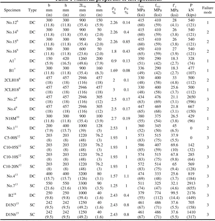
Table 1 – Material properties of test specimens

List of Figures:

Fig.1. Average centroidal strain due to flexure

Fig.2. Spring model of ASFI method

Fig.3. Axial-shear-flexure interactions in ASFI method

Fig.4. A reinforced concrete column subjected to shear and axial loads; a) Concrete principal compression stress pattern, b) Cross section, and c) Stress blocks and strains at two adjacent sections

Fig.5. A reinforced concrete membrane element subject to in-plane stresses

Fig.6. A reinforced concrete in-plane shear element showing average stresses

Fig.7. Stresses and strains relations at the critical flexural section, e.g. bottom end-section in Fig. 4

Fig.8. Shear failure at the ultimate deformation for both shear- and flexure-dominated columns

Fig.9. Presumed curvature distribution for a reinforced concrete column

Fig.10. Comparison of experimental result for specimen No.12 and the ultimate deformation and load obtained from the analytical model

Fig 11. Comparison of experimental and analytical results

Table 1 Material properties of test specimens Specimen Type b mm (in) h mm (in) 2Lin mm (in) Sh mm (in) ρg % ρw % fsyx MPa (ksi) fsyy MPa (ksi) f′c MPa (ksi) P kN (kips) Failure mode No.126 DC 300 (11.8) 300 (11.8) 900 (35.4) 150 (5.9) 2.26 0.14 415 (60) 410 (59) 28 (4.1) 540 (121) 1 No.146 DC 300 (11.8) 300 (11.8) 900 (35.4) 50 (2.0) 2.26 0.4 415 (60) 410 (59) 26 (3.8) 540 (121) 2 No.156 DC 300 (11.8) 300 (11.8) 900 (35.4) 50 (2.0) 2.26 0.85 415 (60) 410 (59) 26 (3.8) 540 (121) 2 No.166 DC 300 (11.8) 300 (11.8) 600 (23.6) 50 (2.0) 1.8 0.43 450 (65) 410 (59) 27 (3.9) 540 (121) 2 A17 DC 150 (5.9) 420 (16.5) 1260 (49.6) 200 (7.9) 0.9 0.13 350 (51) 290 (42) 18.3 (2.7) 328 (74) 1 B17 DC 300 (11.8) 300 (11.8) 900 (35.4) 160 (6.3) 1.69 0.08 336 (49) 290 (42) 18.3 (2.7) 477 (107) 1 2CLH188 DC 457 (18) 457 (18) 2946 (116) 457 (18) 2 0.1 330 (48) 400 (58) 33 (4.8) 500 (112) 2 3CLH188 DC 457 (18) 457 (18) 2946 (116) 457 (18) 3 0.1 330 (48) 400 (58) 25.6 (3.7) 500 (112) 1 No.29 DC 457 (18) 457 (18) 2946 (116) 305 (12) 2.5 0.17 434 (63) 476 (69) 21.1 (3.1) 2650 (596) 3 No.49 DC 457 (18) 457 (18) 2946 (116) 305 (12) 2.5 0.17 447 (65) 469 (68) 21.8 (3.1) 667 (150) 2 N18M10 DC 300 (11.8) 300 (11.8) 900 (35.4) 100 (3.9) 2.7 0.19 380 (55) 375 (54) 26.5 (3.8) 429 (96) 1 No.111 DC 200 (7.9) 400 (15.7) 1000 (39) 128 (5) 2.53 1 360 (52) 345 (50) 45 (6.5) 0 2 C5-00S12 SC 203 (8) 203 (8) 1220 (48) 76.2 (3) 1.93 1 573 (83) 515 (75) 37.9 (5.5) 0 3 C10-05S12 SC 203 (8) 203 (8) 1220 (48) 76.2 (3) 1.93 1 586 (85) 407 (59) 69.6 (10) 142 (32) 3 C10-10S12 SC 203 (8) 203 (8) 1220 (48) 76.2 (3) 1.93 1 574 (83) 515 (75) 67.8 (9.8) 285 (64) 3 C10-20N12 SC 203 (8) 203 (8) 1220 (48) 76.2 (3) 1.93 1 572 (83) 514 (75) 65 (9.4) 569 (128) 3 No.413 DC 400 (15.7) 400 (15.7) 3200 (126) 80 (3.1) 1.57 1.1 474 (69) 333 (48) 25.6 (3.7) 819 (184) 3 No.713 SC 550 (21.6) 550 (21.6) 3300 (130) 90 (3.5) 1.25 1 511 (74) 325 (47) 32.1 (4.6) 2913 (655) 3 B214 DC 250 (9.8) 250 (9.8) 1000 (39.4) 40 (1.6) 2.43 0.4 379 (55) 774 (112) 99.5 (14.4) 2176 (449) 3 D1N315 SC 242 (9.5) 242 (9.5) 1250 (49.2) 40 (1.6) 2.43 0.8 461 (67) 486 (71) 37.6 (5.5) 705 (158) 3 D1N615 SC 242 (9.5) 242 (9.5) 1250 (49.2) 40 (1.6) 2.43 0.8 461 (67) 486 (71) 37.6 (5.5) 1410 (317) 3 Footnotes: DC= double curvature, or with two fixed ends, SC=single curvature, or cantilever, b=width of the section, h= Depth of the section, Lin= length of the column from the inflection point to the end section, Sh= hoop spacing,

ρg=longitudinal reinforcement ratio, ρw= transverse reinforcement ratio, fsyx= longitudinal reinforcement yield stress, fsyy=

transverse reinforcement yield stress, f′c= concrete compression strength , P=axial load, Failure mode 1: shear failure at crack

ε2 < ε’c , Failure mode 2: loss of compression strength ε2 < ε’c , and Failure mode 3: shear-compression failure ε2 = ε’c

εxc2 Centroidal Axis

Neutral Axis

FIG. 1. Average centroidal strain due to flexure

P V M1 M2 V P Ks Kxa Kf Kxf Kxs Ks Kx Kf

Axial-shear model Axial-flexure model

FIG. 2. Spring model of ASFI method

FIG. 3. Axial-shear-flexure interactions in ASFI method

P M V Section 1 Section 2 εxc1 Section 1 Section 2 εxf = 0.5(εxc1−εxc2) 12 l εx=εxa +εxs +εxf Inflection point Moment distribution Inflection Section Flexural Section Axial-shear model V P τs =V/bds τs σx σx=σo=P/bh σx φ h γs εo εxa Lin _τ f τf =M/df bLin M εy Centroidal axis

τ

=

τ

=

τ

Lin h 2 f 1 f

P

V

f Concrete Stress Block at Section i+1 i c f (c) (b)

FIG. 4. A reinforced concrete column subjected to shear and axial Loads; a) Concrete principal compression stress pattern, b) Cross section, and c) Stress blocks and strains

at two adjacent sections

x y σx σy τs Concrete f_c′,ε_c′,f_t′,E_c

Horizontal Reinforcement ρ_x,f ,_syx E_sx Vertical Reinforcement ρ_y,f_syy,E_sy

FIG. 5. A reinforced concrete membrane element subject to in-plane stresses

cxy v sy f sx f cy f cx f c θ 1 c f y σ x σ s τ

FIG. 6. A reinforced concrete in-plane shear element showing average stresses

P b d d ′ s A s A′ P

FIG. 7. Stresses and strains relations at the critical flexural section, e.g. bottom end-section in Fig. 4 c s f Centroid 2 a s ε s ε′ c ε a=β1c s f ′ c f s f

Section Strain Actual

Stresses Equivalent Stresses h φ εo x 23

Specimen No.15 Specimen No.12

FIG. 8. Shear failure at the ultimate deformation for both shear- and flexure-dominated columns

Lin

FIG 9. Presumed curvature distribution for a reinforced concrete column

Lin-h φ

h

a) Up to yield point of tensile steel

φ

b) After yield point of tensile steel

x φ_y x

0 100 200 300 400 0.000 0.005 0.010 0.015 0.020 0.025 0.030 Drift ratio La te ra l lo a d ( k N ) . 0 20 40 60 80 La te ra l Lo a d ( k ip s) Test Results Analysis

FIG 10. Comparison of experimental result for specimen No.126 and the ultimate deformation and load obtained from the analytical model

0 100 200 300 400 0.000 0.050 0.100 Drift ratio La te ra l l o a d (k N ) 0 20 40 60 80 L a te ra l Lo a d (k ip s) Test Results 0 100 200 300 400 0.000 0.050 0.100 0.150 0.200 0.250 Drift ratio La te ra l lo a d ( k N ) 0 20 40 60 80 La te ra l Lo a d ( k ip s) Test Results

Specimen No.146 Specimen No.156

0 100 200 300 400 0.00 0.01 0.02 0.03 0.04 0.05 Drift ratio La te ra l lo a d ( k N ) 0 20 40 60 80 La te ra l Lo a d ( k ip s) Test Results 0 100 200 300 400 0.000 0.020 0.040 0.060 0.080 0.100 Drift ratio La te ra l lo a d ( k N ) . 0 20 40 60 80 L a te ra l Lo a d ( k ip s) Test Results

Specimen No.166 Specimen N18M10

0 50 100 150 200 0.000 0.005 0.010 0.015 0.020 Drift ratio L ate ra l lo ad (k N ) . 0 10 20 30 40 L ate ra l L o ad (k ip s) . Test Results 0 100 200 300 400 0.000 0.005 0.010 0.015 0.020 Drift ratio L ate ra l lo ad ( k N ) . 0 20 40 60 80 La te ra l Lo ad ( k ip s) . Test Results Specimen A17 Specimen B17 0 100 200 300 400 0.00 0.01 0.02 0.03 0.04 0.05 Drift ratio La te ra l l o ad (k N ) . 0 20 40 60 80 L at era l Lo ad (k ip s) . Test Results 0 100 200 300 400 0.000 0.010 0.020 0.030 Drift ratio La te ra l lo a d ( k N ) 0 20 40 60 80 L a te ra l L o a d (k ip s) . Test Results Specimen 2CLH188 Specimen 3CLH188 0 100 200 300 400 0.00 0.01 0.02 0.03 0.04 0.05 0.06 Drift ratio L a te ra l lo a d ( k N ) 0 20 40 60 80 L a te ra l Lo a d ( k ip s) . Test Results 0 100 200 300 400 0.000 0.010 0.020 0.030 0.040 0.050 Drift ratio L ate ra l loa d ( k N ) . 0 25 50 75 L ate ra l L o ad ( k ips ) . Test Results

Specimen No.29 Specimen No.49

0 200 400 600 800 0.000 0.010 0.020 0.030 0.040 0.050 0.060 0.070 Deflection Ratio Lo a d (k N ) 0 40 80 120 160 La te ra l Lo a d ( k ip s) . Test Results 0 100 200 300 400 500 600 0.000 0.010 0.020 0.030 0.040 0.050 0.060 Drift ratio L ate ra l lo ad ( k N ) . 0 25 50 75 100 125 L ate ra l L o ad ( k ip s) . Test Results

Specimen No.111 Specimen B214

0 25 50 75 100 0.000 0.020 0.040 0.060 0.080 0.100 0.120 Drift ratio L ate ra l lo ad ( k N ) . 0 5 10 15 20 L ate ra l L o ad ( k ip s) . Test Results 0 25 50 75 100 125 0.000 0.020 0.040 0.060 0.080 0.100 Drift ratio L ate ra l lo ad ( k N ) . 0 8 16 24 L ate ra l L o ad ( k ip s) . Test Results Specimen C5-00S12 Specimen C10-05S12 0 25 50 75 100 125 0.000 0.020 0.040 0.060 0.080 0.100 Drift ratio L ate ra l loa d ( k N ) . 0 8 16 24 L ate ra l L o ad ( k ips ) . Test Results 0 50 100 150 0.000 0.020 0.040 0.060 0.080 0.100 Drift ratio L ate ra l loa d ( k N ) . 0 8 16 24 32 L ate ra l L o ad ( k ip s) . Test Results Specimen C10-10S12 Specimen C10-20N12 0 50 100 150 200 250 0.000 0.020 0.040 0.060 0.080 0.100 Drift ratio L ate ra l lo ad ( k N ) . 0 10 20 30 40 50 L ate ra l L o ad ( k ip s) . Test Results 0 200 400 600 800 0.000 0.020 0.040 0.060 0.080 Drift ratio L ate ra l lo ad ( k N ) . 0 50 100 150 L ate ra l L o ad ( k ip s) . Test Results

Specimen No.413 Specimen No.713

0 50 100 150 200 250 300 0.000 0.010 0.020 0.030 0.040 0.050 Drift ratio L ate ra l lo ad ( k N ) . 0 20 40 60 L ate ra l L o ad ( k ip s) . Test Results 0 50 100 150 200 250 300 0.000 0.010 0.020 0.030 0.040 0.050 Drift ratio L ate ra l loa d ( k N ) . 0 20 40 60 La te ra l Lo ad (k ip s) . Test Results Specimen D1N315 Specimen D1N615

FIG 11. Comparison of experimental and analytical results

Ultimate drift result of analysis is depicted by