Searches for scalar leptoquarks and differential cross-section measurements in dilepton-dijet events in proton-proton collisions at a centre-of-mass energy of $\sqrt{s}$ = 13 TeV with the ATLAS experiment

EUROPEAN ORGANISATION FOR NUCLEAR RESEARCH (CERN)

Eur. Phys. J. C 79 (2019) 733

DOI:10.1140/epjc/s10052-019-7181-x

CERN-EP-2018-262 17th September 2019

Searches for scalar leptoquarks and differential

cross-section measurements in dilepton–dijet events

in proton–proton collisions at a centre-of-mass

energy of

√

s = 13 TeV with the ATLAS experiment

The ATLAS Collaboration

Searches for scalar leptoquarks pair-produced in proton–proton collisions at √

s= 13 TeV at the Large Hadron Collider are performed by the ATLAS experiment. A data set corresponding to an integrated luminosity of 36.1 fb−1is used. Final states containing two electrons or two muons and two or more jets are studied, as are states with one electron or muon, missing transverse momentum and two or more jets. No statistically significant excess above the Standard Model expectation is observed. The observed and expected lower limits on the leptoquark mass at 95% confidence level extend up to 1.29 TeV and 1.23 TeV for first- and second-generation leptoquarks, respectively, as postulated in the minimal Buchmüller–Rückl– Wyler model, assuming a branching ratio into a charged lepton and a quark of 50%. In addition, measurements of particle-level fiducial and differential cross sections are presented for the Z → ee, Z → µµ and t ¯t processes in several regions related to the search control regions. Predictions from a range of generators are compared with the measurements, and good agreement is seen for many of the observables. However, the predictions for the Z → `` measurements in observables sensitive to jet energies disagree with the data.

© 2019 CERN for the benefit of the ATLAS Collaboration.

Reproduction of this article or parts of it is allowed as specified in the CC-BY-4.0 license.

1 Introduction

Leptoquarks (LQs) are features of a number of extensions of the Standard Model (SM) [1–8] and may provide an explanation for the similarities between the quark and lepton sectors in the SM. They also appear in models addressing some of the recent b-flavour anomalies [9–11]. They are colour-triplet bosons with fractional electric charge and possess non-zero baryon and lepton number [12]. Scalar and vector LQs have been proposed and are expected to decay directly into lepton–quark pairs. The lepton can be either electrically charged or neutral.

A single Yukawa coupling, λLQ→`q, determines the coupling strength between scalar LQs and the lepton–

quark pair [13]. Two additional coupling constants due to magnetic moment and electric quadrupole moment interactions are needed for vector LQs [14].

LQs can be produced both singly and in pairs in proton–proton (pp) interactions; diagrams showing representative single- and pair-production processes are shown in Figure1. The single-LQ production cross-section depends on λLQ→`q whereas the pair-production cross-section is largely insensitive to

this coupling. For pp interactions with a centre-of-mass energy √

s = 13 TeV, gluon fusion represents the dominant pair-production mechanism for LQ masses below around 1 TeV. The contribution of the q ¯q-annihilation process rises with LQ mass. Only scalar LQ production is considered in this paper because this is less model dependent than vector LQ production. The production of vector LQs depends on additional parameters and a full interpretation in such models is beyond the scope of this analysis. The results obtained here can, however, be regarded as conservative estimates of limits on vector LQ production, since the production cross-section for vector LQs is typically much larger than for scalar LQs, while the kinematic properties used to search for their signature are very similar for both spin hypotheses [8].

q

g

l

LQ

g

g

LQ

LQ

Figure 1: Diagrams for representative (a) single and (b) pair production of LQs.

The benchmark signal model used in this paper is the minimal Buchmüller–Rückl–Wyler (BRW) model [15]. This model imposes a number of constraints on the properties of the LQs. Couplings are purely chiral and LQs belong to three families, corresponding to the three SM generations, such that only leptons and quarks within a given generation can interact. The requirement of same-generation interactions excludes flavour-changing neutral currents (FCNC) [16]. The branching ratio (BR) of a LQ into different states is taken as a free parameter. In this paper, β denotes the BR for a LQ decay into a charged lepton and quark, LQ → `±q. The BR for a LQ decay into a neutrino and quark is (1 − β).

This paper presents a search for LQs pair-produced in pp collisions at √

s = 13 TeV, performed by the ATLAS experiment at the Large Hadron Collider (LHC). In previous searches for pair-produced LQs made by ATLAS [17–21], most recently with 3.2 fb−1of data collected at

√

LQs with masses below 1100 (900) GeV for first-generation LQs at β = 1 (0.5) and, for second-generation LQs, with masses below 1050 (830) GeV at β = 1 (0.5) was excluded [21]. Searches have also been made by the CMS Collaboration [22–28] using the same model assumptions as in this work. That experiment found that scalar LQs with masses below 1435 (1270) GeV for first-generation LQs at β = 1 (0.5) and below 1530 (1285) GeV for second-generation LQs at β = 1 (0.5) are excluded at 95% confidence level (CL) using a data sample of 35.9 fb−1collected at

√

s = 13 TeV [27,28]. An overview of limits on LQ production and masses can be found in Ref. [29].

The decay of pair-produced LQs can lead to final states containing a pair of charged leptons and jets, or one charged lepton, a neutrino and jets. For down-type leptoquarks with a charge of 1₃e, assumed here as a benchmark, this can be written more explicitly as LQLQ −→ `−q`+q for the dilepton channel, and¯ LQLQ −→ `−q ¯ν ¯q0or LQLQ −→ νq`+q¯0for the lepton-neutrino channel, respectively. The four search channels in this paper correspond to the above decays. The eejj (µµjj) channel comprises exactly two electrons (muons) and at least two jets, and the eνjj (µνjj) channel requires exactly one electron (muon), missing momentum in the transverse plane and at least two jets. The electron and muon channels are treated separately as they correspond to LQs of different generations. The dilepton and lepton–neutrino channels are combined in order to increase the sensitivity to the parameter of the BRW model, β. While the main target of this paper are first- and second-generation LQs, there are also dedicated searches looking for 3rd generation LQ production [20,30–34].

The main background processes in this search are Z /γ∗+jets, W +jets and t ¯t production. The shapes of these background distributions are estimated from Monte Carlo (MC) simulations while their normalisation is obtained from a simultaneous background-only profile likelihood fit to three data control regions (CRs). The CRs are defined with specific selections such that they are orthogonal to the signal regions (SRs), free from any LQ signal of interest, and enriched in their relevant background process. For the particular benchmark model chosen, further signal and background discrimination could be achieved by exploiting flavour tagging in order to reject events with b-hadrons in the search region. This is not used, in order to maintain sensitivity to a LQ coupling to a b-quark. The shapes and normalisations of other (subdominant) backgrounds are estimated from MC simulation. Background contributions from misidentified leptons are also sub-dominant, and are estimated from data when their contribution is significant.

Several variables that provide separation between signal and background processes are combined into a single discriminant using a boosted decision tree (BDT) method [35]. For each LQ-mass hypothesis and for each lepton flavour, two BDTs are used: one for the dilepton channel and one for the lepton–neutrino channel. The BDT output score is binned and the signal is accumulated at high score values. A single bin at a high score defines the SR for the respective mass hypothesis. The bin range is chosen such that a sensitivity estimator based on the expected number of signal and background events is maximised. A profile likelihood fit is performed simultaneously to both the dilepton and lepton-neutrino channel for each lepton flavour to extract a limit on the signal yield. This is done for different assumptions of LQ mass and branching ratio β, resulting in exclusion bounds in terms of these parameters.

In addition to the search results, this paper presents a set of particle-level fiducial and differential cross-section measurements in six dilepton–dijet regions which are related to the analysis CRs. The measurements are made for the dominant process in each region (Z +jets or t ¯t) exclusively. The motivation for making these measurements is as follows. Search CRs are typically in kinematic regions which are not directly covered by dedicated measurements of SM processes. For instance, the ATLAS measurement of Z + jets production described in Ref. [36] has much looser selections on the transverse momentum (pT) of leptons

ensure that they agree with the available SM data. However, in some cases, although good agreement is seen for the regions covered by dedicated SM measurements, significant disagreements remain possible in more extreme regions where no measurements are available to validate the generator predictions. Indeed, although no disagreement was seen when validating generated Z +jets samples against various SM measurements [37], significant disagreement was observed in the Z +jets CR for this search. Extracting particle-level cross-sections in these CRs and related more extreme regions of phase space can therefore provide complementary information to validate the performance of event generators. Such measurements may lead to improved background modelling in future searches with final states using similar CRs (see for example Ref. [38]).

The paper is organised as follows. Section2gives an overview of the ATLAS detector, while Section3

summarises information on the data set and simulations used. The physics objects used in the analysis are defined in Section4. The background estimation and CRs used in the process are described in Section5, and Section6 provides details on the cross-section extraction. Section7 gives an overview over the multivariate analysis employed for the search and the SRs defined with it. The systematic uncertainties are summarised in Section8, and the statistical procedure employed for the search is described in Section9. Results from both the measurement and the search are given in Section10. Section11concludes the paper.

2 The ATLAS detector

The ATLAS experiment [39] is a multipurpose detector with a forward–backward symmetric cylindrical geometry and nearly 4π coverage in solid angle.1 The three major subcomponents are the tracking detector, the calorimeter and the muon spectrometer. Charged-particle tracks and vertices are reconstructed by the inner detector (ID) tracking system, comprising silicon pixel and microstrip detectors covering the pseudorapidity range |η| < 2.5, and a transition radiation straw-tube tracker that covers |η| < 2.0 and provides electron identification. The ID is immersed in a homogeneous 2 T magnetic field provided by a solenoid. Electron, photon, and jet energies are measured with sampling calorimeters. The calorimeter system covers a pseudorapidity range of |η| < 4.9. Within the region |η| < 3.2, barrel and endcap high-granularity lead/liquid argon (LAr) electromagnetic calorimeters are deployed, with an additional thin LAr presampler covering |η| < 1.8, to correct for energy loss in material upstream of the calorimeters. Hadronic calorimetry is provided by a steel/scintillator-tile calorimeter, segmented into three barrel structures within |η| < 1.7, and two copper/LAr hadronic endcap calorimeters. The forward region (3.1 < |η| < 4.9) is instrumented with a LAr calorimeter with copper (electromagnetic) and tungsten (hadronic) absorbers. Surrounding the calorimeters is a muon spectrometer (MS) with air-core toroid magnets to provide precise muon identification and momentum measurements, consisting of a system of precision tracking chambers providing coverage over |η| < 2.7, and detectors with triggering capabilities over |η| < 2.4. A two-level trigger system [40], the first level using custom hardware and followed by a software-based level, is used to reduce the event rate to a maximum of around 1 kHz for offline storage.

1_{ATLAS uses a right-handed coordinate system with its origin at the nominal interaction point (IP) in the centre of the detector}

and the z-axis along the beam pipe. The x-axis points from the IP to the centre of the LHC ring, and the y-axis points upward. Cylindrical coordinates (r, φ) are used in the transverse plane, φ being the azimuthal angle around the beam pipe. The pseudorapidity is defined in terms of the polar angle θ as η = − ln tan(θ/2). The quantity ∆R =

p

(∆φ)2+ (∆η)2_{is used to}

3 Data and Monte Carlo samples

3.1 Data sample

This analysis is based on proton–proton collision data at a centre-of-mass energy of √

s = 13 TeV, collected at the LHC during 2015 and 2016. After imposing requirements based on beam and detector conditions and data quality, the data sample corresponds to an integrated luminosity of 36.1 fb−1. A set of triggers is used to select events [40–42]. For the dielectron channel, a two-electron trigger with a transverse energy (ET)

threshold of 17 GeV for each electron was used for the entire data set. In the electron–neutrino channel, events were selected by either of two single-electron triggers, as described below. For the 2015 data set, one trigger required ET above 60 GeV. A second trigger with a higher threshold of 120 GeV but looser

identification requirements otherwise was used. For the 2016 data set, the main difference is that the second trigger had a threshold of 140 GeV. The trigger efficiency is at least 95% for electrons above threshold for the kinematic region used in this work.

In the muon channel, the same triggers were used for the µµjj and the µνjj channels. Events were selected by either of two single-muon triggers. For the 2015 data, one trigger required a transverse momentum of at least 26 GeV and applied an isolation criterion. To maintain a high efficiency at high pT, a second

trigger with a threshold of 50 GeV and no further requirements was used. The main difference for the 2016 data set is that slightly different isolation requirements were used for the lower-pTtrigger. The thresholds

were the same as in 2015. For the offline pTvalues considered in this analysis, the trigger efficiencies have

reached their plateau values, which vary between 50% and 80% in the more central detector region and are around 90% for |η| > 1.05. The variation in trigger efficiency is due to local inefficiencies and incomplete detector coverage.

Multiple pp interactions in the same or neighbouring bunch-crossings can lead to many reconstructed vertices in the beam collision of interest. The primary vertex of the event, from which the leptons are required to originate, is defined as that with the largest sum of squared transverse momenta of its associated tracks. Selected events must contain a primary vertex with at least two associated tracks with p_T> 0.4 GeV.

3.2 Signal and background simulations

Samples of simulated events with pair-produced scalar LQs with masses between 200 GeV and 1700 GeV, in steps of 50 GeV up to 1500 GeV and thereafter 100 GeV, were generated at next-to-leading order (NLO) in QCD [43–45] with the MadGraph 2.4.3 [43,46] program using MadSpin [47] for the decay of LQs. In the simulation, leptoquarks with a charge of 1₃e are used. Accordingly, the first generation LQ decays to either a u-quark and an electron, or a d-quark and an electron neutrino. The second generation LQ decays to either a c-quark and a muon or an s-quark and a muon neutrino. The anti-leptoquarks decay into the corresponding anti-particles. The generator output was interfaced with Pythia 8.212 [48] for the event simulation beyond the hard scattering process, i.e. the parton shower, hadronisation and underlying event, collectively referred to as UEPS. The A14 set of tuned parameters (tune) [49] was used for the UEPS modelling. The NNPDF3.0 NLO [50] parton distribution function (PDF) set was used. The coupling

λ_LQ→`q, which determines the LQ lifetime and width [13] was set to

√

4πα, where α is the fine-structure constant. This value corresponds to a LQ full width of about 0.2% of its mass; LQs can thus be considered to decay promptly. Samples were generated for β with a value of 0.5.

Events containing W or Z bosons and associated jets [51] were simulated with the Sherpa 2.2.1 generator [52]. These event samples include off-shell production of the bosons. Matrix elements were calculated in perturbative QCD for up to two partons at NLO and four partons at leading order (LO) using the Comix [53] and OpenLoops [54] matrix element generators. Merging with the Sherpa UEPS model was performed with the ME+PS@NLO method [55]. The NNPDF3.0 PDF set [56] at next-to-next-to-leading order (NNLO) was used. Simulated processes in which a Z boson decays into leptons are hereafter termed Drell–Yan processes.

For the simulation of t ¯t and single-top-quark production in the W t final state and s-channel the Powheg-Box v2 [57–60] generator was used. For the UEPS modelling for the t ¯t samples, Pythia 8.210 was used, with the A14 tune and the NNPDF2.3 LO [61] PDF set. The t ¯t samples used the NNPDF3.0 set in the matrix element calculations, the single-top samples used the CT10 PDF set. Electroweak t-channel single-top-quark events were produced with the Powheg-Box v1 generator. For the generation of single-top samples, the UEPS modelling was done using Pythia 6.428 [62] with the CTEQ6L1 [63] PDF sets and Perugia 2012 [64] tune. The value of the top mass (mt) was set to 172.5 GeV. The EvtGen v1.2.0 [65] program was used for properties of the bottom and charm hadron decays.

Diboson processes with at least one charged lepton in the final state were simulated using the Sherpa 2.1.1 generator. All diagrams with four electroweak vertices were considered. They were calculated for up to one parton at NLO and up to three partons at LO using the Comix and OpenLoops matrix element generators and merged with the Sherpa UEPS model using the ME+PS@NLO prescription. The CT10 PDF set was used in conjunction with dedicated parton shower tuning developed by the Sherpa authors. The generator cross sections, calculated up to NLO, were used.

To model the effect of multiple proton–proton interactions in the same or neighbouring bunches (pile-up), simulated inclusive proton–proton events were overlaid on each generated signal and background event. The pile-up was simulated with Pythia 8.186 using tune A2 [66] and the MSTW2008LO PDF set [67]. Simulated events were corrected using per-event weights to describe the distribution of the average number of interactions per proton bunch-crossing as observed in data.

The detector response to events in the SM background samples was evaluated with the Geant4-based detector simulation [68,69]. A fast simulation employing a parameterisation of calorimeter response [70] and Geant4 for the other detector components was used for the signal samples. The standard ATLAS reconstruction software was used for both simulated and pp data. Furthermore, correction factors, termed scale factors, which were derived from data were applied as event weights to the simulation of the lepton trigger, reconstruction, identification, isolation, and impact parameter selection, and of b-tagging efficiencies.

4 Object definition and event pre-selection

Electrons are reconstructed from ID tracks which are matched to energy clusters found in the electromagnetic calorimeter. The reconstruction efficiency is higher than 97% for candidates with pT greater than 30 GeV.

An object is identified as an electron following requirements made on the quality of the associated track, shower shapes exploiting the longitudinal segmentation of the electromagnetic calorimeter, leakage into the hadronic calorimeter, the quality of the track-to-cluster matching and measurements of transition radiation made with the TRT [71]. The transverse energy of the electron candidates in the ee j j (eν j j) channel must exceed 40 (65) GeV. Only electron candidates in the pseudorapidity region |η| < 2.47 and excluding

the transition region between the barrel and endcap EM calorimeters (1.37 < |η| < 1.52) are used. The electron identification uses a multivariate technique to define different working points of selection efficiency. In the dielectron channel, the ‘medium’ identification working point with an efficiency above 90% for the candidates considered in this analysis is used. To achieve better rejection against jets misidentified as electrons, a tighter selection is used in the electron–neutrino channel. For the electron–neutrino channel, the ‘tight’ identification working point is used with an efficiency of 85% or more for candidates with pT

above 65 GeV. The electrons are required to be isolated, using both calorimeter- and track-based criteria such that the isolation efficiency is 98%. Finally, the electron candidates have to be compatible with originating from the primary vertex.

Muon tracks are reconstructed independently in the ID and the MS [72]. Tracks are required to have a minimum number of hits in each system, and must be compatible in terms of geometrical and momentum matching. Information from both the ID and MS is used in a combined fit to refine the measurement of the momentum of each muon over |η| < 2.5 [73]. The efficiency for reconstructing muons is 98%. As for the electron channels, muon candidates are required to have pT > 40 GeV and pT > 65 GeV for the

µµjj and µνjj searches respectively. They are further required to be compatible with originating from the primary vertex. A track-based isolation requirement is applied to the muons, yielding a selection efficiency of 99%.

Jets are reconstructed using the anti-ktalgorithm [74] with a radius parameter R = 0.4 from topological clusters of calorimeter cells which are noise-suppressed and calibrated to the electromagnetic scale. They are calibrated using energy- and η-dependent correction factors derived from simulation and with residual corrections from in situ measurements [75]. The jets must satisfy pT> 60 GeV and |η| < 2.5. Additional

jet quality criteria are also applied to remove fake jets caused by detector effects [76]. Furthermore, to eliminate jets containing a large energy contribution from pile-up, jets are tested for compatibility with the hard scatter vertex with a jet vertex tagger discriminant, utilising information from the ID tracks associated with the jet [77].

Jets containing b-hadrons (b-jets) are identified with an algorithm which is based on multivariate techniques. The algorithm combines information from the impact parameters of displaced tracks and from topological properties of secondary and tertiary decay vertices reconstructed within the jet. A working point at which the b-tagging efficiency is around 77% for jets originating from a b-quark is chosen, as determined with a MC simulation of t ¯t processes [78,79]. Scale factors needed to match the MC performance to data are compatible with unity [80].

The missing transverse momentum is defined as the negative vector transverse momentum sum of the reconstructed and calibrated physics objects, plus an additional soft term [81,82]. The soft term is built from tracks that are not associated with any reconstructed electron, muon or jet, but which are associated with the primary vertex. The absolute value of the missing transverse momentum is denoted by E_Tmiss. In the `ν j j channel, an E_Tmiss-related quantity, calculated as S = E_Tmiss/

q pj1 T + p j2 T + p ` T is used to further

reduce backgrounds from objects wrongly reconstructed as leptons. Here, p_Tj1 (p_Tj2) is the pTof the leading

(subleading) jet and p`_Tis the pTof the charged lepton.

Ambiguities in the object identification which arise during reconstruction, i.e. when a reconstructed object can match multiple object hypotheses (electron, muon, jet), are resolved in several steps. First, electrons are removed if they share a track with a muon. An algorithm is also used to remove jet–lepton ambiguities based on the proximity of identified leptons and jets.

For the dilepton channel, events are selected such that they contain at least two jets and two same-flavour leptons fulfilling the requirements above for the respective flavour. Selected lepton-neutrino events have to contain at least two jets, one lepton, and a missing transverse energy of more than 40 GeV.

5 Control regions and background estimation

The major SM background processes to the LQ signal correspond to the production of (off-shell) Z /γ∗+jets, W +jets and t ¯t events in which at least one top quark decays leptonically. These backgrounds are determined using data in selected CRs, as described below. Subdominant contributions arising from diboson, single-top, W → τν and Z → ττ production are estimated entirely from simulation. There are also background contributions due to objects being misidentified as leptons or non-prompt leptons that are produced in the decay of hadrons. These backgrounds are collectively referred to as the fake (lepton) background and are estimated in a data-driven way where relevant.

Three CRs, independent of the SRs used for the leptoquark search (see Section 7), in which any high-mass LQ signal contributions are expected to be negligible are defined in order to estimate the main backgrounds. First, the Z /γ∗+jets control region (Z CR) in the dilepton channels is defined by restricting the dilepton invariant mass, m``, to values between 70 GeV and 110 GeV. These CRs contain samples of Z /γ∗+jets events of purity 92% (94%) for the electron (muon) channel. Next, the W control region (W CR) in the lepton–neutrino channels requires the transverse mass2, mT, to be between 40 GeV and 130 GeV. In

addition, E_Tmisshas to be greater than 40 GeV and the observable S greater than 4. Events that contain one or more b-jets are vetoed to reduce the t ¯t contribution. The purity of the W CR is 74% (80%) for the electron (muon) channel.

To improve the description of data, a reweighting of the Z /γ∗+jets and W +jets predictions by Sherpa 2.2.1 is performed. The weights in this procedure are parameterised as a function of the dijet mass, mj j, in the respective CR, and applied to both CRs and SRs (see Section7). The parameterisation is derived by fitting the ratio between data and prediction with second-degree polynomials. Figure2shows distributions of m_{j jand leading jet pTin the Z CR for the µµjj channel before and after reweighting. The data are better} described by the Monte Carlo simulations following this reweighting. The total uncertainty (statistical, systematic and theory) is shown. The total uncertainty for CR distributions is dominated by the uncertainty in the theoretical predictions which is correlated between bins. Experimental uncertainties from jet energy scale and jet energy resolution are typically around 1%. Similarly, the Sherpa 2.2.1 predictions of W +jets require reweighting to match the data. The functional form of the reweighting algorithm is similar to that used for the Z /γ∗+jets sample. The signal regions differ from the control regions mainly by the cut on m``

or mT. It is verified that applying weights derived in one mass region to the MC simulation in a different

mass region provides a good description of the data in that region, indicating that the same correction is also valid in the signal region. All mass regions used in this test do not overlap with the signal regions. A systematic uncertainty is included to account for the reweighting procedure (Section8).

In the statistical method used to evaluate the exclusion limits which is described in Section 9, the normalisations of background estimates are adjusted in the fitting procedure. These normalisations are not applied to any of the distributions shown prior to that section. Finally, the t ¯t control region (t ¯t CR) for the µνjj and eνjj channels is defined with the same requirements on mTand E_Tmissas the W CR, but here the

2_{The transverse mass is defined as m}

T=

q

2 · p`<sub>T</sub>· E<sub>T</sub>miss· (1 − cos(∆φ(`, E_Tmiss))) where ∆φ(`, E_Tmiss) is the azimuthal separation between the charged lepton and the E_Tmiss.

Events / 200 GeV 2 − 10 1 − 10 1 10 2 10 3 10 4 10 5 10 _ATLAS -1 13 TeV, 36.1 fb jj, Z CR µ µ Data Z(µµ) t t VV tW tot. unc. [GeV] jj m 0 2000 4000 6000 8000 Data / Pred. 0.5 1.0 1.5 (a) Events / 200 GeV 1 − 10 1 10 2 10 3 10 4 10 5 10 ATLAS -1 13 TeV, 36.1 fb jj, Z CR µ µ Data Z(µµ) t t VV tW tot. unc. [GeV] j, lead T p 0 500 1000 1500 2000 Data / Pred. 0.5 1.0 1.5 (b) Events / 200 GeV 2 − 10 1 − 10 1 10 2 10 3 10 4 10 ATLAS -1 13 TeV, 36.1 fb jj, Z CR µ µ Data Z(µµ) t t VV tW tot. unc. [GeV] jj m 0 2000 4000 6000 8000 Data / Pred. 0.5 1.0 1.5 (c) Events / 200 GeV 1 − 10 1 10 2 10 3 10 4 10 5 10 ATLAS -1 13 TeV, 36.1 fb jj, Z CR µ µ Data Z(µµ) t t VV tW tot. unc. [GeV] j, lead T p 0 500 1000 1500 2000 Data / Pred. 0.5 1.0 1.5 (d)

Figure 2: Distributions of mj j (left) and leading jet pT(right) in the Z CR for the µµjj channel. Data are shown

together with MC contributions corresponding to Z → µµ, t ¯t, diboson (VV ) and single-top (tW ) processes. The MC distributions are cumulatively stacked. The bottom panels show the ratio of data to expected background. The grey hatched band represents the total uncertainty. The Sherpa 2.2.1 predictions for Z → µµ are shown before (top) and after (bottom) the reweighting procedure (see text).

presence of at least two b-jets is required. The purity of the t ¯t CR is 86% (89%) for the electron (muon) channel. The CRs are summarised in Table1. The Z CRs and other measurement regions are used to extract particle-level differential cross-sections (see Section6).

This analysis makes use of the matrix method [83] to estimate the background from misidentified electrons for the first-generation LQ search. This background is negligible for the second generation search. The matrix method is based on the estimation of the probabilities for prompt electrons and fake electron candidates that pass identification and isolation selections that are looser than the nominal selection described in Section 4, to also pass the nominal selection. These probabilities are referred to as the

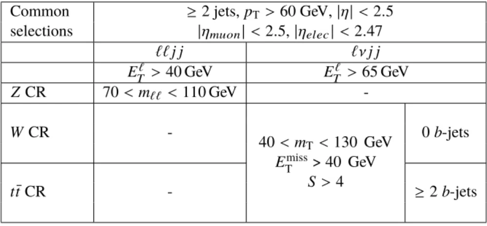
Table 1: Definition of the CRs used in the dilepton and lepton–neutrino channel, respectively. Selections common to both channels are shown at the top.

Common selections ≥ 2 jets, pT > 60 GeV, |η| < 2.5 |ηmuon| < 2.5, |ηelec|< 2.47 `` j j `ν j j E<sub>T</sub>` > 40 GeV E<sub>T</sub>` > 65 GeV Z CR 70 < m`` < 110 GeV -W CR -40 < mT < 130 GeV Emiss T > 40 GeV S> 4 0 b-jets t ¯t CR - ≥ 2 b-jets

prompt rate and fake rate, respectively. In the loose selection, several criteria that are used to suppress fake contributions in the nominal selection are relaxed. In particular, no isolation is required in the loose selection. The prompt rate is estimated to a good approximation from MC simulations, while the fake rate is estimated from a data sample enriched in fake backgrounds. To suppress contributions from prompt electrons in this sample, events are rejected if they contain at least two electron candidates that pass the ‘medium’ identification criteria. In both channels, events are also rejected if there are two electron candidates that fulfil the ‘loose’ object definition specific to the respective channel and have an invariant mass in an interval of ±20 GeV around the Z boson mass. The contribution from the fake electron background is at most 24%, but generally much less.

Backgrounds with non-prompt muons arise from decays of heavy-flavour hadrons inside jets. Their contribution to the dimuon final states is negligible as in the search documented in Ref. [84]. In lepton– neutrino final states, a contamination of about 5% was found [83], corresponding to about half the size of the fake electron background. Tests showed that a contamination of 5% would not alter the results of this analysis, and therefore this background is neglected. The uncertainty in the total background estimation due to neglecting this background is taken to be half the size of the background from fake electrons. In Figure3, the distributions of mmin_LQ and the dilepton invariant mass in the Z CR are shown for the µµjj and eejj channels. The quantities m_LQminane mmax_LQ are defined as the lower and higher of the two invariant masses which can be reconstructed using the two lepton–jet pairs in the dilepton channels. In the analysis, the lepton–jet pairing is chosen such that the absolute mass difference between the two LQ candidates is minimised. The full set of experimental and theoretical uncertainties is considered for the uncertainty band. The spectra correspond to the predictions prior to the fit described in Section9.

Distributions for the eνjj and µνjj channels are similarly shown for the W and t ¯t CRs in Figures 4and 5, respectively. The E_Tmissand mTspectra are shown in Figure4, while the mj j and mTspectra are shown in

Figure5. The data and the predictions in the various CRs are in agreement within uncertainties (described in Section8) following the reweighting of the Sherpa 2.2.1 predictions for Z /γ∗+jets and W +jets processes. After the reweighting, the overall normalisation of the simulation is in very good agreement with the data in the V +jets CRs.

Events / 100 GeV 1 − 10 1 10 2 10 3 10 4 10 5 10 ATLAS -1 13 TeV, 36.1 fb eejj, Z CR Data Z(ee) t t Fake VV tW tot. unc. [GeV] min LQ m 0 1000 2000 3000 Data / Pred. 0.5 1.0 1.5 (a) Events / 3 GeV 10 2 10 3 10 4 10 5 10 6 10 ATLAS -1 13 TeV, 36.1 fb eejj, Z CR Data Z(ee) t t Fake VV tW tot. unc. [GeV] ee m 70 80 90 100 110 Data / Pred. 0.5 1.0 1.5 (b) Events / 100 GeV 1 − 10 1 10 2 10 3 10 4 10 5 10 _ATLAS -1 13 TeV, 36.1 fb jj, Z CR µ µ Data ) µ µ Z( t t VV tW tot. unc. [GeV] min LQ m 0 1000 2000 3000 Data / Pred. 0.5 1.0 1.5 (c) Events / 3 GeV 10 2 10 3 10 4 10 5 10 6 10 ATLAS -1 13 TeV, 36.1 fb jj, Z CR µ µ Data Z(µµ) t t VV tW tot. unc. [GeV] µ µ m 70 80 90 100 110 Data / Pred. 0.5 1.0 1.5 (d)

Figure 3: Distributions of m_LQminand m``in the Z CR for the eejj (top) and µµjj (bottom) channels. Data are shown together with background contributions corresponding to t ¯t, diboson (VV ), Z → ee, Z → µµ, single-top (tW ) processes, and fake electrons. The background distributions are cumulatively stacked. The bottom panels show the ratio of data to expected background. The grey hatched band represents the total uncertainty. A reweighting as a function of mj j is applied to the Z +jets simulation. The other MC predictions are not reweighted.

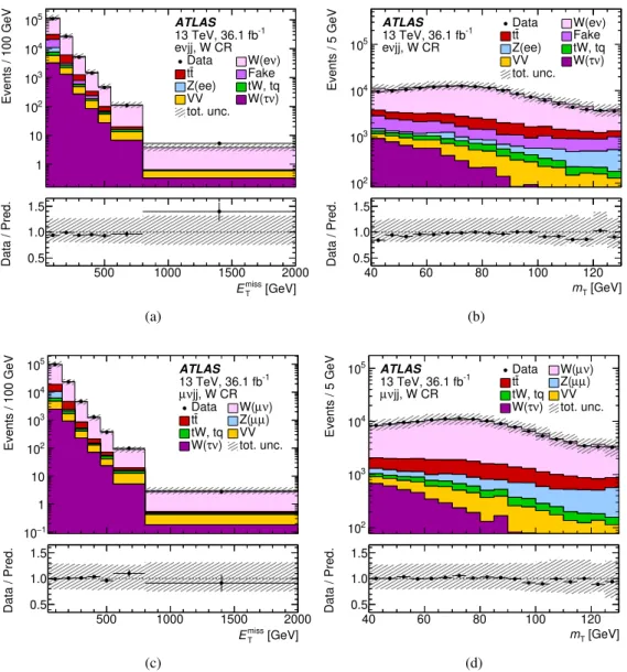
Events / 100 GeV 1 10 2 10 3 10 4 10 5 10 ATLAS -1 13 TeV, 36.1 fb jj, W CR ν e Data W(eν) t t Fake Z(ee) tW, tq VV W(τν) tot. unc. [GeV] miss T E 500 1000 1500 2000 Data / Pred. 0.5 1.0 1.5 (a) Events / 5 GeV 2 10 3 10 4 10 5 10 ATLAS -1 13 TeV, 36.1 fb jj, W CR ν e Data W(eν) t t Fake Z(ee) tW, tq VV W(τν) tot. unc. [GeV] T m 40 60 80 100 120 Data / Pred. 0.5 1.0 1.5 (b) Events / 100 GeV 1 − 10 1 10 2 10 3 10 4 10 5 10 ATLAS -1 13 TeV, 36.1 fb jj, W CR ν µ Data W(µν) t t Z(µµ) tW, tq VV ) ν τ W( tot. unc. [GeV] miss T E 500 1000 1500 2000 Data / Pred. 0.5 1.0 1.5 (c) Events / 5 GeV 2 10 3 10 4 10 5 10 ATLAS -1 13 TeV, 36.1 fb jj, W CR ν µ Data W(µν) t t Z(µµ) tW, tq VV ) ν τ W( tot. unc. [GeV] T m 40 60 80 100 120 Data / Pred. 0.5 1.0 1.5 (d)

Figure 4: Distributions of E_Tmissand mTin the W CR for the eνjj (top) and µνjj (bottom) channels. Data are shown

together with background contributions corresponding to t ¯t, diboson (VV ), Z → ee, Z → µµ, W → µν, W → eν, W →τν, single-top production (tW, tq) processes, and fake electrons. The background distributions are cumulatively stacked. The bottom panels show the ratio of data to expected background. The grey hatched band represents the total uncertainty. A reweighting as a function of mj j is applied to the W +jets and Z +jets simulation. The other MC predictions are not reweighted.

Events / 200 GeV 1 − 10 1 10 2 10 3 10 4 10 5 10 6 10 ATLAS -1 13 TeV, 36.1 fb CR t jj, t ν e Data tt ) ν W(e Fake Z(ee) tW, tq VV W(τν) tot. unc. [GeV] jj m 0 2000 4000 6000 8000 Data / Pred. 0.5 1.0 1.5 (a) Events / 5 GeV 10 2 10 3 10 4 10 5 10 6 10 ATLAS -1 13 TeV, 36.1 fb CR t jj, t ν e Data tt ) ν W(e Fake Z(ee) tW, tq VV W(τν) tot. unc. [GeV] T m 40 60 80 100 120 Data / Pred. 0.5 1.0 1.5 (b) Events / 200 GeV 1 − 10 1 10 2 10 3 10 4 10 ATLAS -1 13 TeV, 36.1 fb CR t jj, t ν µ Data tt ) ν µ W( Z(µµ) tW, tq VV ) ν τ W( tot. unc. [GeV] jj m 0 2000 4000 6000 8000 Data / Pred. 0.5 1.0 1.5 (c) Events / 5 GeV 10 2 10 3 10 4 10 5 10 ATLAS -1 13 TeV, 36.1 fb CR t jj, t ν µ Data tt ) ν µ W( Z(µµ) tW, tq VV ) ν τ W( tot. unc. [GeV] T m 40 60 80 100 120 Data / Pred. 0.5 1.0 1.5 (d)

Figure 5: Distributions of mj j and mTin the t ¯t CR for the eνjj (top) and µνjj (bottom) channels. Data are shown

together with background contributions corresponding to t ¯t diboson (VV ), Z → ee, Z → µµ, W → µν, W → eν W →τν, single-top production (tW, tq) processes, and fake electrons. The background distributions are cumulatively stacked. The bottom panels show the ratio of data to expected background. The grey hatched band represents the total uncertainty. A reweighting as a function of mj jis applied to the Z +jets and W +jets simulations. The other MC predictions are not reweighted.

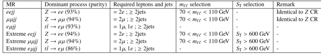
Table 2: Requirements at particle-level for all measurement regions (MRs) where particle-level differential cross-sections are extracted. The purity refers to the proportion of the particle-level yield of the MR which is accounted for by the dominant process. The variable STrefers to the scalar sum of the pTof the jets and leptons.

MR Dominant process (purity) Required leptons and jets m``selection STselection Remark

eejj Z → ee (93%) = 2e ; ≥ 2jets 70 < m``< 110 GeV - Identical to Z CR µµjj Z →µµ (94%) = 2µ ; ≥ 2jets 70 < m``< 110 GeV - Identical to Z CR eµjj t ¯t → eµ (93%) = 1µ, 1e ; ≥ 2jets - -

-Extreme eejj Z → ee (94%) = 2e ; ≥ 2jets 70 < m``< 110 GeV ST> 600 GeV

-Extreme µµjj Z →µµ (94%) = 2µ ; ≥ 2jets 70 < m``< 110 GeV ST> 600 GeV

-Extreme e µjj t ¯t → eµ (86%) = 1µ, 1e ; ≥ 2jets - ST> 600 GeV

-6 Extraction of particle-level cross-sections from the measurement regions

Measurements of the particle-level fiducial and differential cross-sections are made in several regions related to the search CRs described in the previous section. These measurement regions (MRs) correspond to kinematic regions where new physics signals have already been excluded. They are chosen because several searches with related final states use similar selections for their CRs (see for example Ref. [38]).

6.1 Particle-level objects

In order to extract fiducial and differential cross-sections in the MRs, particle-level object selections are defined, and chosen to be as close as possible to their detector-level counterparts described in Section4. Prompt dressed3particle-level electrons and muons are used to define the fiducial region. They are required to have pT > 40 GeV and |η| < 2.5.

Particle-level jets are formed by clustering stable4particles using the anti-kt (R = 0.4) algorithm [74], excluding muons and neutrinos. Particle-level jets are required to have pT > 60 GeV and |η| < 2.5.

The electrons used in the jet clustering are not dressed. To match the requirements of the detector-level jet-lepton ambiguity resolution procedure, any particle-level leptons within ∆R < 0.4 from a selected jet are removed.

6.2 Measurement region definitions

The first two MRs are identical to the eejj and µµjj Z CRs described in Table1. The third is an e µjj region where the leptons are required to have different flavours, and no requirement on the dilepton mass is applied. Finally, three additional regions are defined as for the eejj, µµjj and e µjj MRs, and labelled as extreme with the additional requirement that the scalar sum of the pTof the leptons and the two leading jets (ST) be

above 600 GeV. The requirements for events entering all MRs are summarised in Table2.

The MRs are defined both at detector level and particle level, where the requirements are identical but use the objects passing the detector-level and particle-level selections respectively. The mj j reweighting is also applied to events from the simulated Drell–Yan sample at particle level, where the particle-level value of m_{j jis used to calculate the weight. In each MR, the cross-section measurements are made for dominant}

3_{Dressed leptons are obtained by adding the four-vectors of all photons found within a cone of size ∆R = 0.1 around the lepton.}

Photons from hadron decays are excluded.

processes. The contributions from all other processes are subtracted from the data yield, as explained in Section6.3.

6.3 Particle-level measurement method

Each MR is designed such that it is dominated by a single SM process (accounting for more than 85% of the yield, see Table2), for which the cross-section can be measured exclusively. A simple procedure to extract particle-level cross-sections, based on bin-by-bin correction factors, is used. In this method, the particle-level differential cross-section for the dominant process p in bin i of the distribution of variable X can be expressed as:

dσ_ip dX = (Ni−Íq,pR q i) · T_ip R_ip wi· L , ₍₁₎

where the sum runs over all sub-dominant SM processes which contribute to the yield, Niis the number of events observed in the bin, R_ip(T_ip) is the yield at detector level (particle level) for process p, wiis the width of the bin and L is the integrated luminosity of the data sample. The bin-by-bin correction factors T_ip/R_ip may be thought of as the inverse of the reconstruction efficiency in bin i, assuming no bin-by-bin migrations. The bin-by-bin correction procedure doesn’t account for migration between bins due to resolution effects when going from particle-level to detector-level distributions. For this reason, the binning of the distributions is chosen to be much broader than the experimental resolution to minimise the migration between bins. This binning is optimised for the measurements to ensure that at least 90% of events passing the particle-level selection remain in the same bin at detector level (for events passing both selections). This binning is not used for the search.

Differential cross-section measurements are made for the following observables: pTof the dilepton system;

∆φ between the leptons; minimum ∆φ between lepton and leading jet; minimum ∆φ between lepton and subleading jet; ST; leading jet pT; subleading jet pT; ∆φ and ∆η between the leading and subleading jets;

scalar sum of pTof leading and subleading jets (HT); and invariant mass of the dijet system.

7 Multivariate analysis and signal regions

In order to discriminate between signal and background in the LQ search, the TMVA [35] implementation of a BDT is used. A number of variables are expected to provide discrimination between signal and background. Generally, the pTof the leptons and jets as well as related variables such as STwill possess

higher values for the signal than for the background, in particular for high LQ mass. Since the signature arises from the decay of parent LQs with well-defined masses, mass-sensitive discriminating variables are further candidates for BDT input variables. In the dilepton channels, the lepton-jet masses mmin_LQ and mmax_LQ are reconstructed, as described in Section5. In the lepton–neutrino channels, the mass of one LQ (mLQ)

and the transverse mass of the second LQ (m_LQT ) can be reconstructed. The transverse mass is defined as mT

LQ =

q

2 · p_Tj · E_Tmiss· (1 − cos(∆φ( j, E_Tmiss))), where ∆φ( j, E_Tmiss) is the azimuthal angle between the jet and the direction of missing transverse momentum vector. The procedure is analogous to that used in the dilepton channel; both possible pairings of jet and lepton (or E_Tmiss) are tested and the pairing that results in the smaller absolute difference between mLQand m_LQT is chosen.

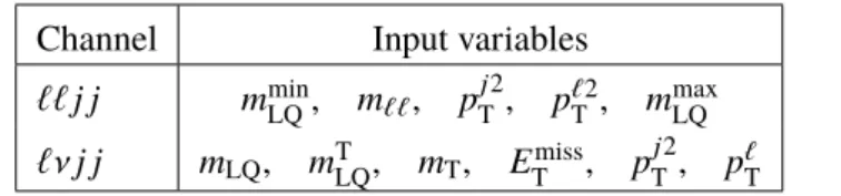
Table 3: BDT input variables in the dilepton and lepton–neutrino channels.

Channel Input variables

`` j j mmin LQ, m``, p j2 T , p `2 T , m max LQ `ν j j m_LQ, mT LQ, mT, E miss T , p j2 T , p ` T

All background processes are used in the BDT training. For the electron and muon channels separately, the training is done for each LQ mass hypothesis for which signal simulations were produced. To ensure independence from the CRs, in the dilepton channel, only events with a dilepton invariant mass above 130 GeV are considered in the training. Similarly, only events with a transverse mass greater than 130 GeV are considered in the lepton–neutrino channel. Here, to further suppress the fake-electron contribution, it is required that E_Tmiss> 150 GeV and that S > 3. These requirements define the training regions (TRs), i.e. event samples used to train the BDTs.

To ensure that no bias is introduced, two BDTs are used for each mass point; one is trained on one half of the events and evaluated on the other half, and vice versa for the second BDT. Different methods of dividing the simulation samples into training and test samples are tested and compared, giving consistent results such that no overtraining or other biases are introduced in the process.

Table3lists the variables that were found to give optimal sensitivity, ordered by their discriminating power in the BDT. In the dilepton channel, these are both reconstructed LQ candidate masses, mmin_LQ and mmax_LQ, the dilepton invariant mass, m``, the subleading jet pT (p

j2

T) and the subleading lepton pT (p `2 T ). The

lepton–neutrino channel also makes use of both of the LQ mass variables, mLQand mT_LQ, and the other

variables are the transverse mass, mT, the missing transverse momentum, E_Tmiss, the subleading jet pT,

and the charged-lepton pT, p`_T. Distributions of a selection of the variables used for training are shown

in AppendixB. It was checked and confirmed that not only the individual input variables but also their pairwise correlations are modelled well in the simulation.

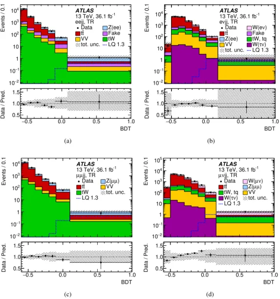
Output distributions for the BDT discriminant in the TRs are shown in Figure6for a signal sample of LQ mass 1.3 TeV. The background distributions are shown before the fit (see Sec.9). The contribution of a LQ of mass 1.3 TeV, normalised to the production cross-section, is also shown for the four channels. The background includes the reweighted predictions of Z /γ∗+jets and W +jets. An increased separation between signal and background at higher values of the BDT output is seen.

The SR phase-space is a subset of that considered in the TRs. The same object and event selections as in the TRs are made in the SRs, but in addition a requirement is placed on the BDT score. As stated above, each BDT is trained on half of the events in the TR and evaluated on the other half, and the obtained BDT score distribution is used to determine the SR. In this way, the SR determined based on a given BDT does not overlap with the TR used for that BDT. For the dilepton and lepton–neutrino channels separately, the SRs are defined as a single bin in the output score distribution of the respective BDT. The bin range is determined for each mass point separately by maximising the quantity [85] Z =p(s+ b) log(1 + s/b) − s, where s and b are the signal and background expectations, respectively. In this optimisation, a number of further requirements are placed on the background expectations: there have to be at least two background events in the chosen region; the statistical uncertainty of the number of background events estimated by the simulation has to be less than 20%; if less than ten background events are expected, the statistical uncertainty is required to be less than 10%. This is done to avoid selecting bins with very low background expectation and thus to increase the fit stability.

Events / 0.1 2 − 10 1 − 10 1 10 2 10 3 10 4 10 ATLAS -1 13 TeV, 36.1 fb eejj, TR Data Z(ee) t t Fake VV tW tot. unc. LQ 1.3 BDT 0.5 − 0.0 0.5 1.0 Data / Pred. 0.5 1.0 1.5 (a) Events / 0.1 2 − 10 1 − 10 1 10 2 10 3 10 4 10 ATLAS -1 13 TeV, 36.1 fb jj, TR ν e Data W(eν) t t Fake Z(ee) tW, tq VV W(τν) tot. unc. LQ 1.3 BDT 0.5 − 0.0 0.5 1.0 Data / Pred. 0.5 1.0 1.5 (b) Events / 0.1 2 − 10 1 − 10 1 10 2 10 3 10 4 10 ATLAS -1 13 TeV, 36.1 fb jj, TR µ µ Data Z(µµ) t t VV tW tot. unc. LQ 1.3 BDT 0.5 − 0.0 0.5 1.0 Data / Pred. 0.5 1.0 1.5 (c) Events / 0.1 2 − 10 1 − 10 1 10 2 10 3 10 4 10 5 10 _ATLAS -1 13 TeV, 36.1 fb jj, TR ν µ Data W(µν) t t Z(µµ) tW, tq VV ) ν τ W( tot. unc. LQ 1.3 BDT 0.5 − 0.0 0.5 1.0 Data / Pred. 0.5 1.0 1.5 (d)

Figure 6: Output distributions for the BDT in the training regions (TRs) for the four search channels: (a) eejj (b) eνjj (c) µµjj and (d) µνjj. Data are shown together with pre-fit background contributions corresponding to t ¯t, diboson (VV ), Z → ee, Z → µµ, W → µν, W → eν, W → τν, single-top production (tW , tq) processes, and fake electrons. The prediction for a LQ with mass 1.3 TeV is also shown. The predicted background distributions are cumulatively stacked. The bottom panels show the ratio of data to expected background. The grey hatched band represents the total uncertainty.

In total, there are 58 SRs in the electron and the muon channel each: two SRs (`` j j and `ν j j) for each of the 29 mass hypotheses considered. The fraction of signal events that is left after acceptance selections and losses due to detector inefficiencies, is estimated from the simulation to rise from less than 1% at low masses (around 200 GeV) to 60–70% for masses around 1500 GeV.

8 Systematic uncertainties

The systematic uncertainties for the search are divided into two categories: experimental uncertainties and theoretical uncertainties in the background and the signal. Most of the sources of uncertainties are common to both the search and the measurement. In addition to the common set of uncertainties, the measurement incorporates MC modelling uncertainties from closure tests. The search applies uncertainties to normalisation factors of the major backgrounds and their extrapolation to the SRs; these are evaluated in the CR-only profile likelihood fit in which the normalisation factors are determined. In Sections8.1and8.2, the sources of experimental and theoretical uncertainies are outlined, respectively. The impact of the major uncertainties on the search and the measurements are described in Sections8.3and8.4, respectively.

8.1 Experimental uncertainties

The uncertainty in the combined 2015+2016 integrated luminosity is 2.1%. It is derived, following a methodology similar to that detailed in Ref. [86], and using the LUCID-2 detector for the baseline luminosity measurements [87], from calibration of the luminosity scale using x–y beam-separation scans. An uncertainty due to the reweighting of the vertex multiplicity to describe pile-up is estimated by scaling the average number of interactions per bunch-crossing in data by different factors.

The major sources of uncertainties affecting the electron measurement derive from the electron energy scale and resolution measurements. The analysis also considers uncertainties due to the modelling of the efficiencies of the four electron selection criteria: trigger, reconstruction, identification and isolation. Sources of experimental uncertainties related to muon reconstruction and calibration include uncertainties in the determination of the MS momentum scale, MS momentum resolution, ID momentum resolution and additional charge-dependent corrections. Furthermore, uncertainties in the determination of the four efficiency scale factors, introduced at the end of Section 3.2, for trigger, identification, isolation and track-to-vertex matching are taken into account.

There are two main sources of uncertainty related to the jet reconstruction: jet energy scale (JES) and jet energy resolution (JER). Another source of jet-related uncertainty corresponds to corrections made for the b-tagging efficiency. The uncertainty due to the JES is largely derived from various in situ techniques. Four components of this uncertainty are considered.

The uncertainties due to the electron, muon and jet energy scale and resolution are propagated to the estimation of E_Tmiss. In addition, there is an uncertainty from the soft term, which has three components: one corresponding to the E_Tmissscale and two components for the E_Tmissresolution uncertainty. The resolution uncertainty is split into components parallel and perpendicular to an axis in the transverse plane which is defined along the direction of a vectorial sum of all the hard objects in the event (electrons, muons and jets).

An uncertainty in the fake rate of electrons is determined by varying the MC prediction that is used to remove the contributions of prompt electrons from the fake-enriched sample by 30%. The effect is propagated to the fake background estimate. The uncertainty due to neglecting the muon fake background is taken to be half the size of the electron fake background, see Section5.

8.2 Theoretical uncertainties

The Sherpa 2.2.1 V +jets samples include event weights reflecting variations of the nominal PDF set (NNPDF3.0) and the use of two different PDF sets: MMHT2014NNLO68CL [88] and CT14NNLO [89]. The NNPDF intra-PDF uncertainty is estimated as the standard deviation of the set of 101 NNPDF3.0 eigenvectors. This procedure takes into account the effect of varying αSby ±0.001 around its nominal

value of 0.119. The envelope of the differences between the nominal NNPDF set and the other two PDF sets is used as an additional uncertainty.

The samples include weights for seven sets of variation of the renormalisation (µr) and factorisation (µf)

scale, i.e. varying the scales up and down by a factor of two, either together or independently. The envelope of all these variations is taken as an estimate of the scale uncertainty.

A further uncertainty from the reweighting of the V +jets simulations in mj j is considered. The full difference between the reweighted and the unweighted distributions is taken as an estimate of the uncertainty induced by the reweighting.

The uncertainties in the modelling of the production of t ¯t are assessed from a number of alternative simulation samples. Differences between different generators and different models for fragmentation and hadronisation are considered. In addition, parameters affecting initial- and final-state radiation are also varied. For the t ¯t sample the default PDF set is NNPDF3.0 and the PDF uncertainty is estimated from the PDF4LHC15 prescription [90].

8.3 Uncertainties for the search

As described in Section9three CRs are fit simultaneously to obtain normalisation factors. Sources of theoretical uncertainty described above are taken into account in this procedure. Furthermore, theory uncertainties in the SRs correspond to variations in the output BDT spectra and are thus taken into account in the final limit setting calculation.

The electron energy scale and reconstruction affect the total background yield in the SRs for the electron channels by 2–14%. Similarly uncertainties due to the muon reconstruction and calibration lead to background uncertainties of between 2 and 20% for the muon channels. The impact of uncertainties related to the JES (JER) lead to uncertainties on the predicted background of 5–20% (2–20%). The effect of the soft-term uncertainties in the E_Tmissestimations leads to variations of the background estimate from less than 1% to 15%. Generally, the experimental uncertainties in the signal yields in the SRs are not larger than 2%.

Uncertainties of approximately 100% for the fake electron background are estimated at low values of lepton-jet mass in the TR and about 20% at masses above 1 TeV. The statistical uncertainty in the electron fake rate determination is below 10%. As discussed earlier, the contribution from fake muons is typically half the size of the electron fake background, and this is used as a (conservative) estimate of the uncertainty in the total background due to neglecting the muon fake contribution.

The final modelling uncertainties in the background yields for Z +jets and W +jets are around 2–10%, with the scale uncertainty typically being the dominant source. Signal predictions have an uncertainty of a similar size. The background from t ¯t production is affected by a theoretical unceratinty of up to 50%, the large value arising due to the statistical imprecision of the MC samples.

8.4 Uncertainties for the cross-section measurements

The uncertainties described below are those which apply to the particle-level cross-section measurements in the MRs, in addition to the relevant uncertainties from the previous sections. As is described in Section6, the cross-section calculation involves the subtraction of non-dominant processes from the observed data, and the application of bin-by-bin correction factors. The experimental uncertainties play a role in both of these steps, since they affect the detector-level yield of both the non-dominant processes (when subtracting from data) and the dominant process (when calculating the correction factors). The dominant experimental uncertainties are the JES and the lepton efficiencies, which have effects of up to 5% and 2% on the fiducial cross-sections respectively. Theory and modelling uncertainties in the dominant process affect both the particle-level and detector-level yields, and therefore largely cancel out when calculating the correction factors T /R (see Eq.1).

The theory uncertainties in the dominant processes in the Z +jets and t ¯t MRs therefore have only a small impact (≤ 2%) on the fiducial cross-sections. The theory uncertainties in the estimation of non-dominant processes generally have a minimal impact since these processes usually account for only small fractions of the MR yield. The exception is the case of the t ¯t background to the Z MRs, which also contribute a small but non-negligible theory uncertainty.

In addition, bin-by-bin correction uncertainties are derived by comparing the nominal correction factors with those obtained using re-weighted V +jets and alternative t ¯t samples. The size of these modelling uncertainties ranges between 0.5% and 4% of the fiducial cross-sections.

The overall uncertainty of the fiducial cross-sections, accounting for all sources of systematic uncertainty, is between 5% and 9% depending on the MR.

9 Statistical procedure for the search

The results of the analysis are interpreted using a profile likelihood method as implemented in Histfitter [91], in particular using the asymptotic formulae from Ref [85]. The signal and backgrounds are described by a binned probability density function (p.d.f.) built using either the three CRs described in Section5, or the two SRs, one in the dilepton channel and one in the lepton–neutrino channel, as described in Section7. All CRs and SRs consist of only a single bin.

The CRs are enriched in a specific background process and have a negligible signal contamination; they are thus used to normalise the predicted backgrounds to data, whereas the SRs drive the signal extraction. The p.d.f. for the fit to the SRs includes the signal strength, i.e. the scaling factor with respect to the predictions for the signal cross-section, as the parameter of interest. Systematic uncertainties are incorporated in the p.d.f. as statistical nuisance parameters. They are introduced as shape uncertainties, i.e. they can only affect the relative size of a given background in different regions while preserving the overall number of expected events. This is done in order to remove strong correlations with the normalisation factors for

the main backgrounds that are extracted from the CRs and which are used to scale MC yields to match data. Experimental uncertainties are treated as being fully correlated between different physics processes and fit regions. Theoretical or modelling uncertainties are treated as correlated in different fit regions, but uncorrelated between processes. The statistical uncertainties of the MC samples are included in the p.d.f. as nuisance parameters by constraint terms described by a Γ distribution. . The fit is performed in two stages: first, only the CRs are included in the fit in order to extract the normalisation factors for the three main backgrounds. These normalisation factors are then applied to the main backgrounds in the second step, which is a fit to only the SRs. The uncertainty in the normalisation factors from the CR fit is introduced in the form of Gaussian nuisance parameters. The best-fit central values and constraints on other nuisance parameters are not transferred from the CRs to the SRs. The optimal value and error of the signal strength and nuisance parameters as well as their correlations are determined simultaneously when the p.d.f. is fitted to data. This conservative two-step approach is chosen for its simplicity compared with the case of a simultaneous fit to all regions.

For some systematic uncertainties, certain adjustments are made before they are incorporated in the fit, as described in the following. Uncertainties larger than 50% are capped at 50%, because their large size is due to the statistical uncertainty of simulation samples used to estimate them. This applies in particular to the theoretical uncertainties in the t ¯t estimation. Uncertainties with very asymmetric up and down variations are symmetrised, using the larger of the two variations. In the SR fit, experimental uncertainties that before normalisation have an effect smaller than 2% on the total background or the signal expectation are not considered in the fit for the background or the signal, respectively. Other nuisance parameters are not considered for certain background processes if their effect is less than 2% on that process before normalising the uncertainty.

10 Results

10.1 Results of the cross-section measurements

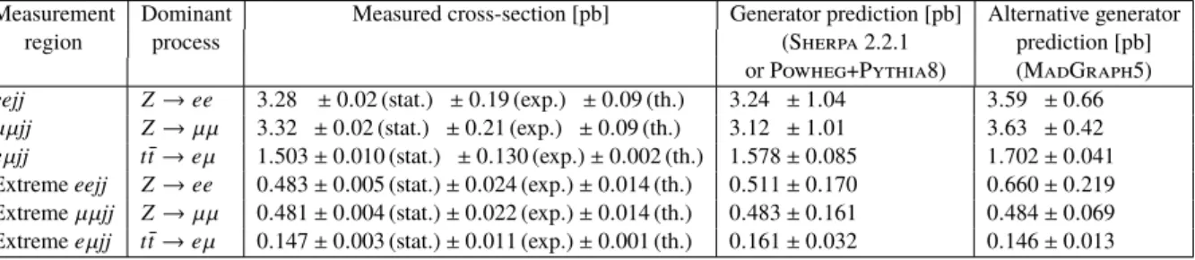
The measured fiducial particle-level cross-sections are shown in Table4for each of the six MRs. The values in all MRs are found to agree with the generator predictions within uncertainties. The uncertainties in the measured cross-sections are in all cases dominated by experimental uncertainties (in particular the jet energy scale). The theory uncertainties in the generator predictions are dominated by variations in the cross-sections, arising from QCD scale variations in the phase-space regions of the measurements. In both the standard and extreme MRs, the measured fiducial cross-sections in the Z MRs are found to agree between electron and muon decay modes, as expected.

Examples of the particle-level differential cross-sections are shown in Figures7and8, where they are compared with the cross-sections predicted from the nominal simulation without the mj j reweighting. Predictions from alternative generators are also shown in each case. Differential cross-sections for a larger list of variables are included in AppendixAand in the HEPData [92,93] record for this paper [94]. In the eejj and µµjj MRs (and their extreme counterparts) the predicted differential cross-sections for variables involving jet energies exhibit a degree of mis-modelling by the Sherpa 2.2.1 simulation. This can be seen in Figures 7and 8, for the leading jet pT as an example. Similar mis-modelling is seen

for mj j, HT, subleading jet pT, and ST differential measurements. All other quantities are shown to be

well modelled by the nominal Sherpa 2.2.1 simulation. In all cases, the prediction of an alternative generator, MadGraph5_aMC@NLO (with events generated at NLO accuracy for Z + 0, 1, 2 jets, showered

Table 4: Measured fiducial cross-section for the dominant process in each of the MRs, with uncertainties broken down into the statistical, experimental, and theoretical components. The generator predictions with their uncertainties are obtained from Sherpa 2.2.1 for the Z → ee and Z → µµ samples, and Powheg+Pythia8 for the t ¯t sample. Alternative generator predictions are also provided, obtained using MadGraph5 FxFx and MadGraph5+Pythia8 for the Z MRs and t ¯t MRs, respectively.

Measurement Dominant Measured cross-section [pb] Generator prediction [pb] Alternative generator region process (Sherpa 2.2.1 prediction [pb]

or Powheg+Pythia8) (MadGraph5)

eejj Z → ee 3.28 ± 0.02 (stat.) ± 0.19 (exp.) ± 0.09 (th.) 3.24 ± 1.04 3.59 ± 0.66 µµjj Z →µµ 3.32 ± 0.02 (stat.) ± 0.21 (exp.) ± 0.09 (th.) 3.12 ± 1.01 3.63 ± 0.42 eµjj t ¯t → eµ 1.503 ± 0.010 (stat.) ± 0.130 (exp.) ± 0.002 (th.) 1.578 ± 0.085 1.702 ± 0.041 Extreme eejj Z → ee 0.483 ± 0.005 (stat.) ± 0.024 (exp.) ± 0.014 (th.) 0.511 ± 0.170 0.660 ± 0.219 Extreme µµjj Z →µµ 0.481 ± 0.004 (stat.) ± 0.022 (exp.) ± 0.014 (th.) 0.483 ± 0.161 0.484 ± 0.069 Extreme e µjj t ¯t → eµ 0.147 ± 0.003 (stat.) ± 0.011 (exp.) ± 0.001 (th.) 0.161 ± 0.032 0.146 ± 0.013

using Pythia8 with the A14 tune, and for which different jet multiplicities were merged using the FxFx prescription [95]), is also shown. Typically, the MadGraph5_aMC@NLO prediction is also discrepant with the data for the same observables, but often in a direction opposite to that of the Sherpa 2.2.1 prediction. This suggests that the discrepancies are caused by choices of the generator parameters, which would have been tuned in a different phase-space region given by previous Z + jets measurements. The measurements provided by this paper will therefore help to validate new tunes of the generators to ensure better agreement in this region for future searches. These disagreements in modelling are covered by the reweighting uncertainty when evaluating limits for the search.

For the e µjj MRs, the predictions from the nominal Powheg simulation are found to agree with the data for all observables aside from the dilepton pT, where a slight mis-modelling is observed in the high tail,

as can be seen in the examples shown in Figures7and8. The predictions of an alternative generator (MadGraph5_aMC@NLO) are also shown, and these do agree with the data for this observable. This points to the generator tuning choice as the source of the disagreement.

6 − 10 5 − 10 4 − 10 3 − 10 2 − 10 1 − 10 1 500 1000 1500 2000 2500 0.5 1 1.5 ATLAS -1 fb TeV, 36.1 13 eejj [GeV] T j Leading p ) [pb/GeV] T j / d(p σ d Pred. / Data Data Statistical error Sherpa2.2.1 MG5_aMC+Py8 FxFx 0 0.5 1 1.5 2 2.5 3 3.5 4 0 0.5 1 1.5 2 2.5 3 0.7 1 1.3 ATLAS -1 fb TeV, 36.1 13 eejj l)[rad] 0 (j φ ∆ min l)) [pb/rad]₀ (j φ∆ / d(min σ d Pred. / Data Data Statistical error Sherpa2.2.1 MG5_aMC+Py8 FxFx 6 − 10 5 − 10 4 − 10 3 − 10 2 − 10 1 − 10 1 500 1000 1500 2000 2500 0.5 1 1.5 ATLAS -1 fb TeV, 36.1 13 jj µ µ [GeV] T j Leading p ) [pb/GeV] T j / d(p σ d Pred. / Data Data Statistical error Sherpa2.2.1 MG5_aMC+Py8 FxFx 0 0.5 1 1.5 2 2.5 3 3.5 4 0 0.5 1 1.5 2 2.5 3 0.7 1 1.3 ATLAS -1 fb TeV, 36.1 13 jj µ µ l)[rad] 0 (j φ ∆ min l)) [pb/rad]₀ (j φ∆ / d(min σ d Pred. / Data Data Statistical error Sherpa2.2.1 MG5_aMC+Py8 FxFx 6 − 10 5 − 10 4 − 10 3 − 10 2 − 10 1 − 10 500 1000 1500 2000 2500 0.5 1 1.5 ATLAS -1 fb TeV, 36.1 13 jj µ e [GeV] T j Leading p ) [pb/GeV] T j / d(p σ d Pred. / Data Data Statistical error Powheg+Py8 MG5_aMC+Py8 5 − 10 4 − 10 3 − 10 2 − 10 1 − 10 1 0 200 400 600 800 1000 1200 1400 1600 1800 2000 0.4 1 1.6 ATLAS -1 fb TeV, 36.1 13 jj µ e [GeV] T µ e p ) [pb/GeV] T µ e / d(p σ d Pred. / Data Data Statistical error Powheg+Py8 MG5_aMC+Py8

Figure 7: Examples of the measured particle-level differential cross-sections in the eejj, µµjj and e µjj measurement regions, exclusively for the dominant process in each channel (Z → ee, Z → µµ and t ¯t, respectively). The MC prediction for the dominant process is also shown, with no mj jreweighting applied. The red band represents the statistical component of the total uncertainty on the measurement which is indicated by the error bar on each point. The variable min∆Φ( j0, l) refers to the minimal difference in φ between the leading jet and a prompt lepton.

6 − 10 5 − 10 4 − 10 3 − 10 2 − 10 1 − 10 500 1000 1500 2000 2500 0.5 1 1.5 ATLAS -1 fb TeV, 36.1 13 Extreme eejj [GeV] T j Leading p ) [pb/GeV] T j / d(p σ d Pred. / Data Data Statistical error Sherpa2.2.1 MG5_aMC+Py8 FxFx 0 0.2 0.4 0.6 0.8 1 0 0.5 1 1.5 2 2.5 3 0.6 1 1.4 ATLAS -1 fb TeV, 36.1 13 Extreme eejj l)[rad] 0 (j φ ∆ min l)) [pb/rad]₀ (j φ∆ / d(min σ d Pred. / Data Data Statistical error Sherpa2.2.1 MG5_aMC+Py8 FxFx 6 − 10 5 − 10 4 − 10 3 − 10 2 − 10 1 − 10 500 1000 1500 2000 2500 0.5 1 1.5 ATLAS -1 fb TeV, 36.1 13 jj µ µ Extreme [GeV] T j Leading p ) [pb/GeV] T j / d(p σ d Pred. / Data Data Statistical error Sherpa2.2.1 MG5_aMC+Py8 FxFx 0 0.1 0.2 0.3 0.4 0.5 0.6 0.7 0.8 0.9 0 0.5 1 1.5 2 2.5 3 0.6 1 1.4 ATLAS -1 fb TeV, 36.1 13 jj µ µ Extreme l)[rad] 0 (j φ ∆ min l)) [pb/rad]₀ (j φ∆ / d(min σ d Pred. / Data Data Statistical error Sherpa2.2.1 MG5_aMC+Py8 FxFx 6 − 10 5 − 10 4 − 10 3 − 10 2 − 10 500 1000 1500 2000 2500 0.5 1 1.5 ATLAS -1 fb TeV, 36.1 13 jj µ Extreme e [GeV] T j Leading p ) [pb/GeV] T j / d(p σ d Pred. / Data Data Statistical error Powheg+Py8 MG5_aMC+Py8 5 − 10 4 − 10 3 − 10 2 − 10 0 200 400 600 800 1000 1200 1400 1600 1800 2000 0.3 1 1.7 ATLAS -1 fb TeV, 36.1 13 jj µ Extreme e [GeV] T µ e p ) [pb/GeV] T µ e / d(p σ d Pred. / Data Data Statistical error Powheg+Py8 MG5_aMC+Py8

Figure 8: Examples of the measured particle-level differential cross-sections in the extreme eejj, µµjj and e µjj measurement regions, exclusively for the dominant process in each channel (Z → ee, Z → µµ and t ¯t, respectively). The MC prediction for the dominant process is also shown, with no mj jreweighting applied. The red band represents the statistical component of the total uncertainty on the measurement which is indicated by the error bar on each point. For the leading jet pTmeasurement, the uncertainty in the second bin is smaller because the bin-by-bin correction

factor from the alternative t ¯t samples agrees more closely with the nominal ones than in neighbouring bins. The variable min∆Φ( j0, l) refers to the minimal difference in φ between the leading jet and a prompt lepton.